
Large-Scale LiDAR SLAM with Factor Graph Optimization on High-Level Geometric Features


Abstract
1. Introduction
- robust data association methods for creation of and updating the planar and linear features,
- efficient map management procedures that make it possible to build large, feature-based maps,
- loop closing using robust descriptors for loop detection and geometric features for map optimization,
- thorough evaluation of the proposed solution in different variants and in several representative scenarios.
2. Related Work
2.1. Architectures of LiDAR-Based SLAM
2.2. Scan Registration Methods
2.3. Closing Loops in LiDAR SLAM
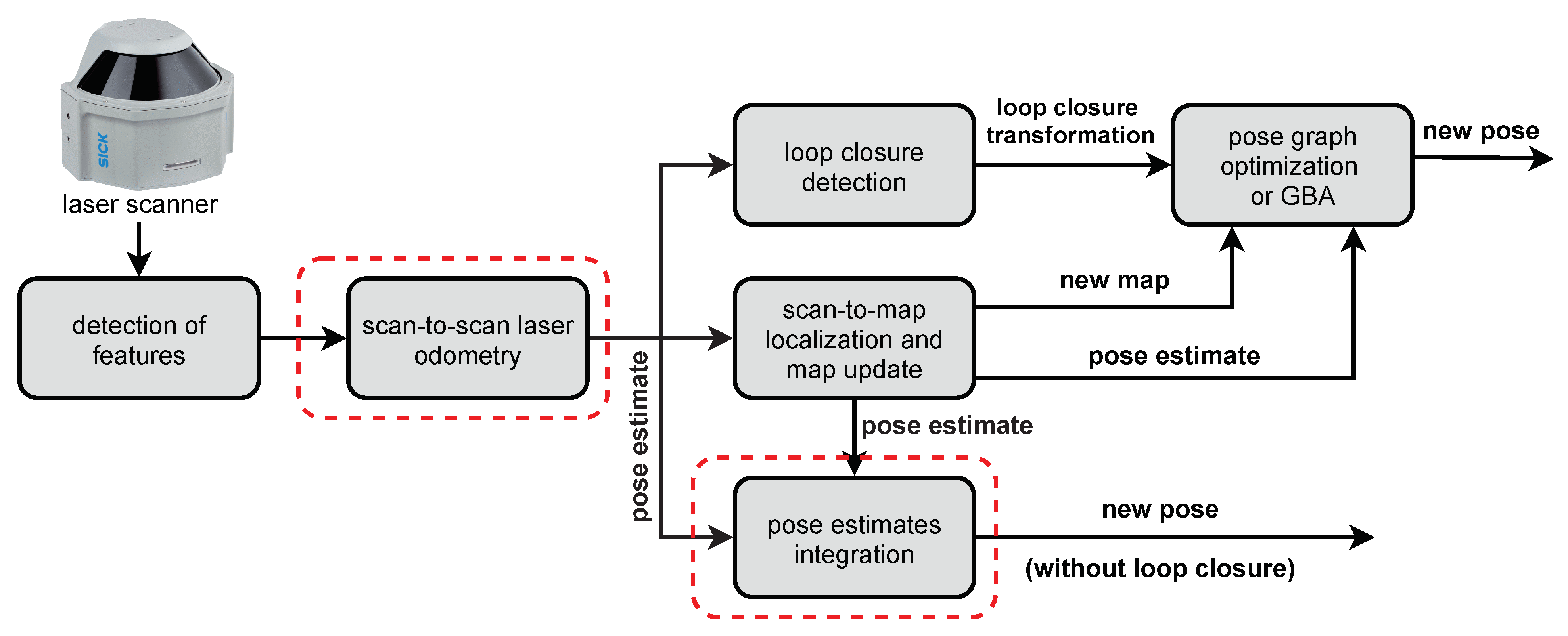
3. The Architecture of PlaneLOAM
3.1. Odometry
- Velodyne HDL-64E:where is a horizontal angle of the i-th measurement, is a horizontal angle of the start of the scan, and is a horizontal angle of the end of the scan
- Sick MRS 6124:where g is a number of a scanning ring, counting from the top.
- Ouster OS1-64:where i is an index of the measurement.
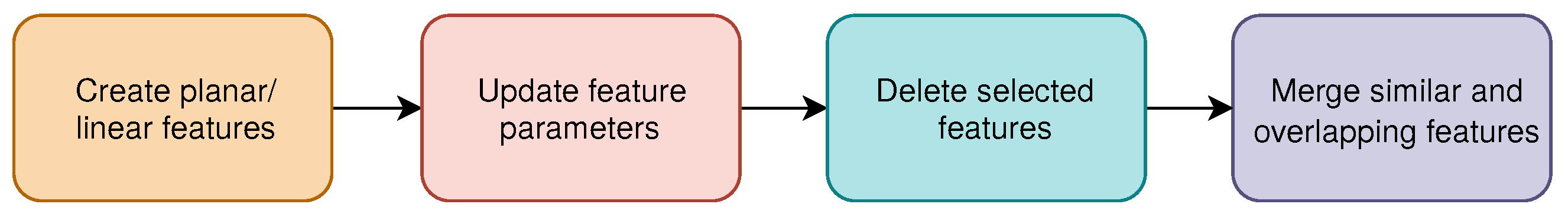
3.2. Mapping
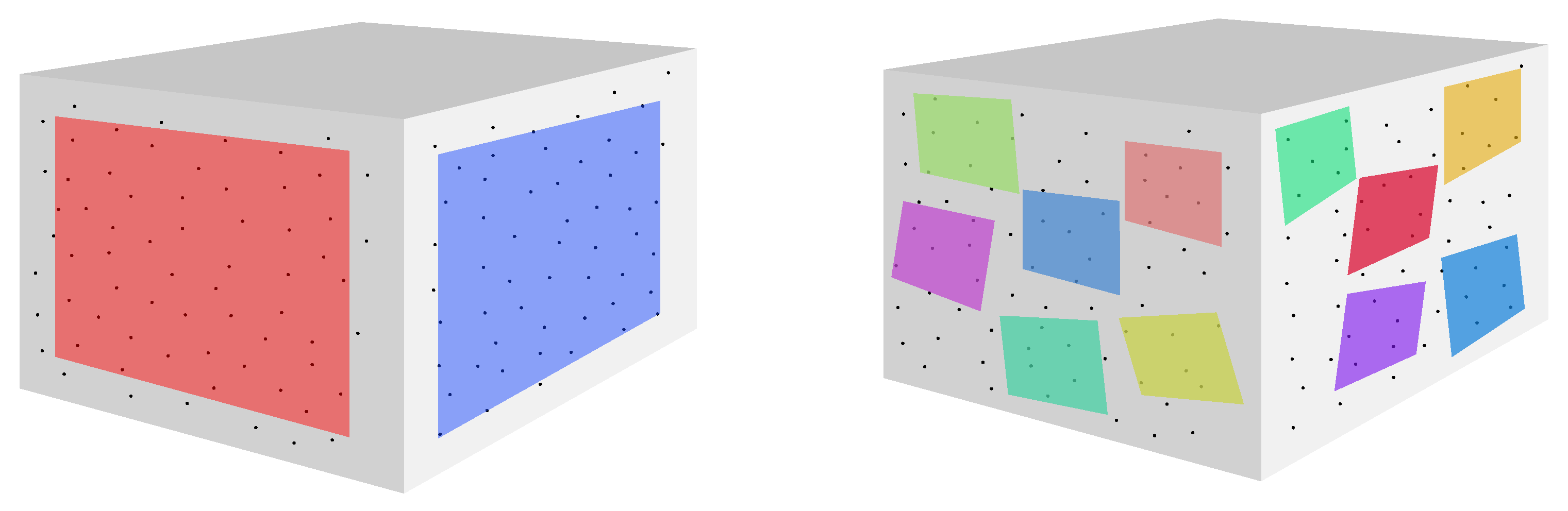
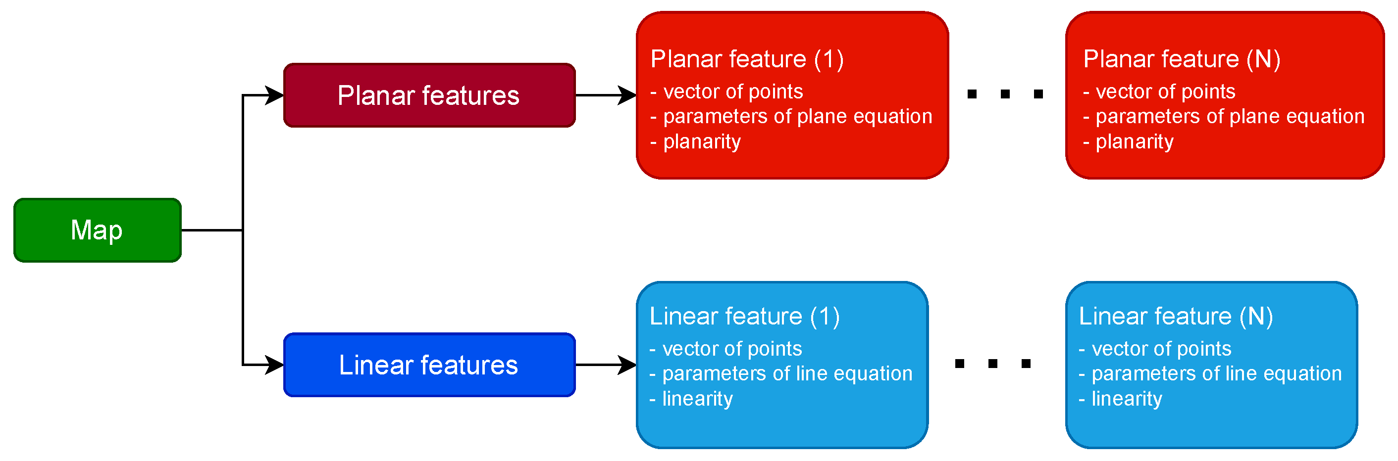
3.2.1. Map Representation
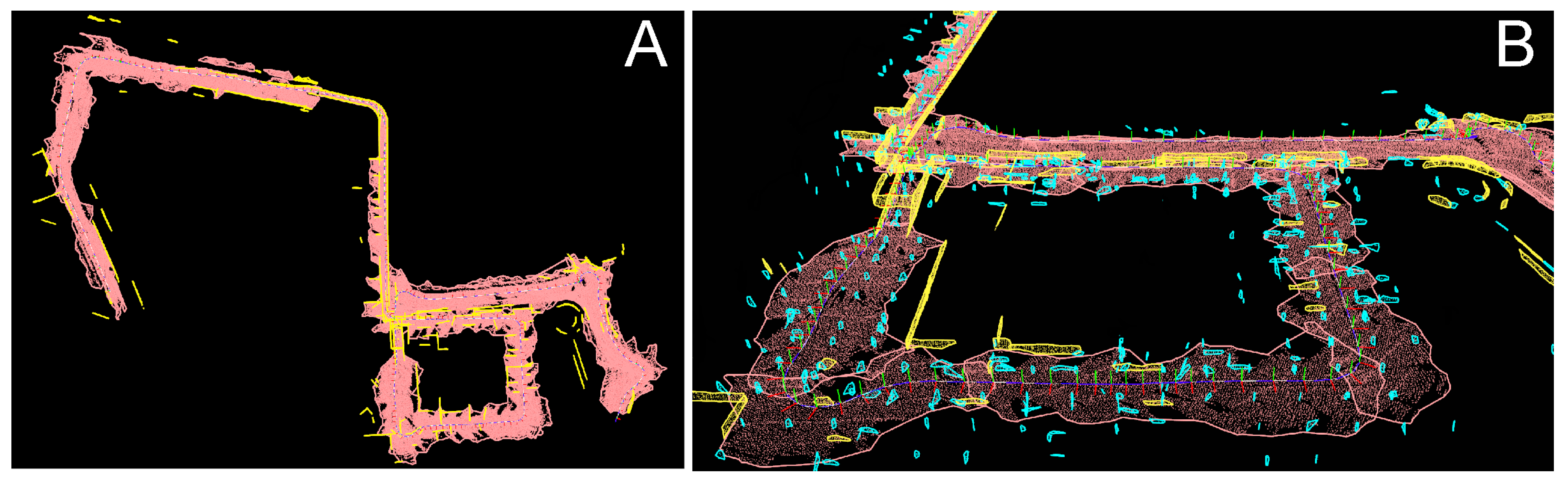
3.2.2. Creating Features
3.2.3. Updating and Deleting Features
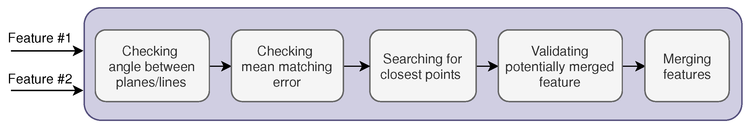
3.2.4. Merging Features
3.2.5. Pose Estimation
3.2.6. Parameters in Mapping
4. Loop Closing
4.1. Loop Closing Detection
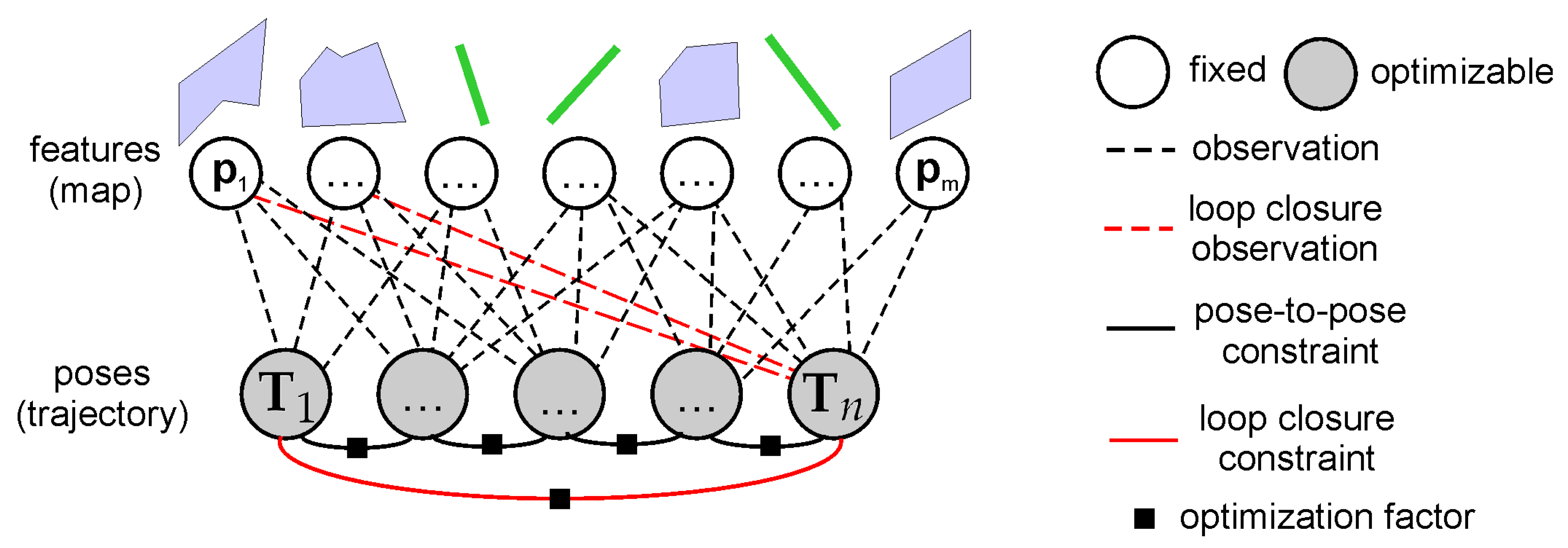
4.2. Pose Graph Optimization
4.3. Loop Closure Based on Map Features
4.3.1. Plane Representation for Optimization
4.3.2. Minimal Line Representation
- —we use a series expansion of ;
- —we avoid the issue by performing computation with equivalent Plücker representation ( and );
- —we set and follow the conversion with a new random, unit-length vector of that is perpendicular to . As , the random choice of has no impact on Plücker coordinates obtained from the minimal representation.
5. Experimental Evaluation
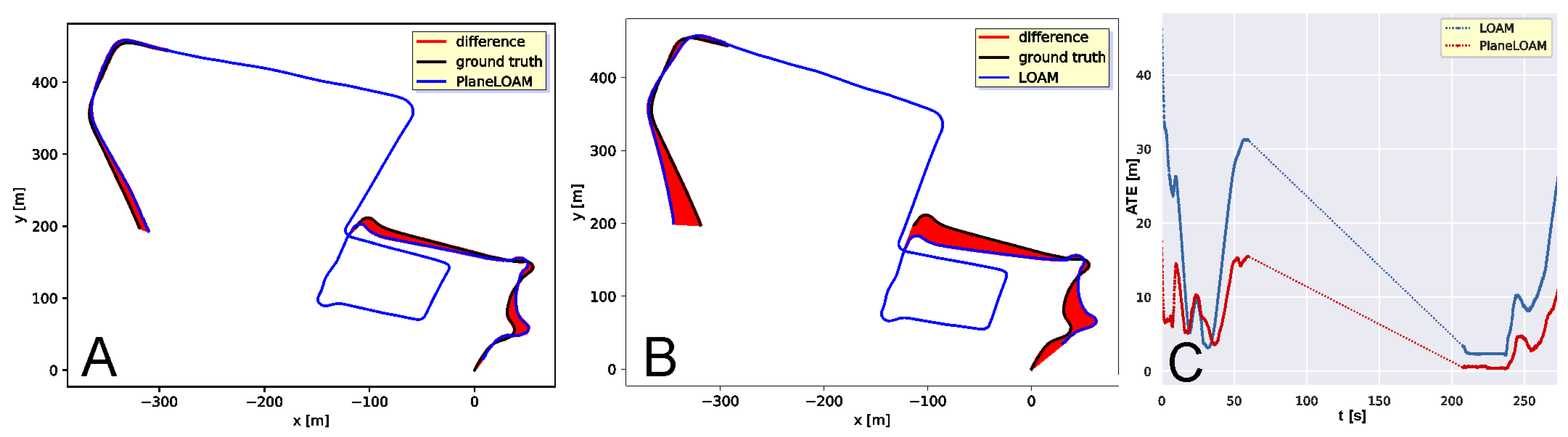
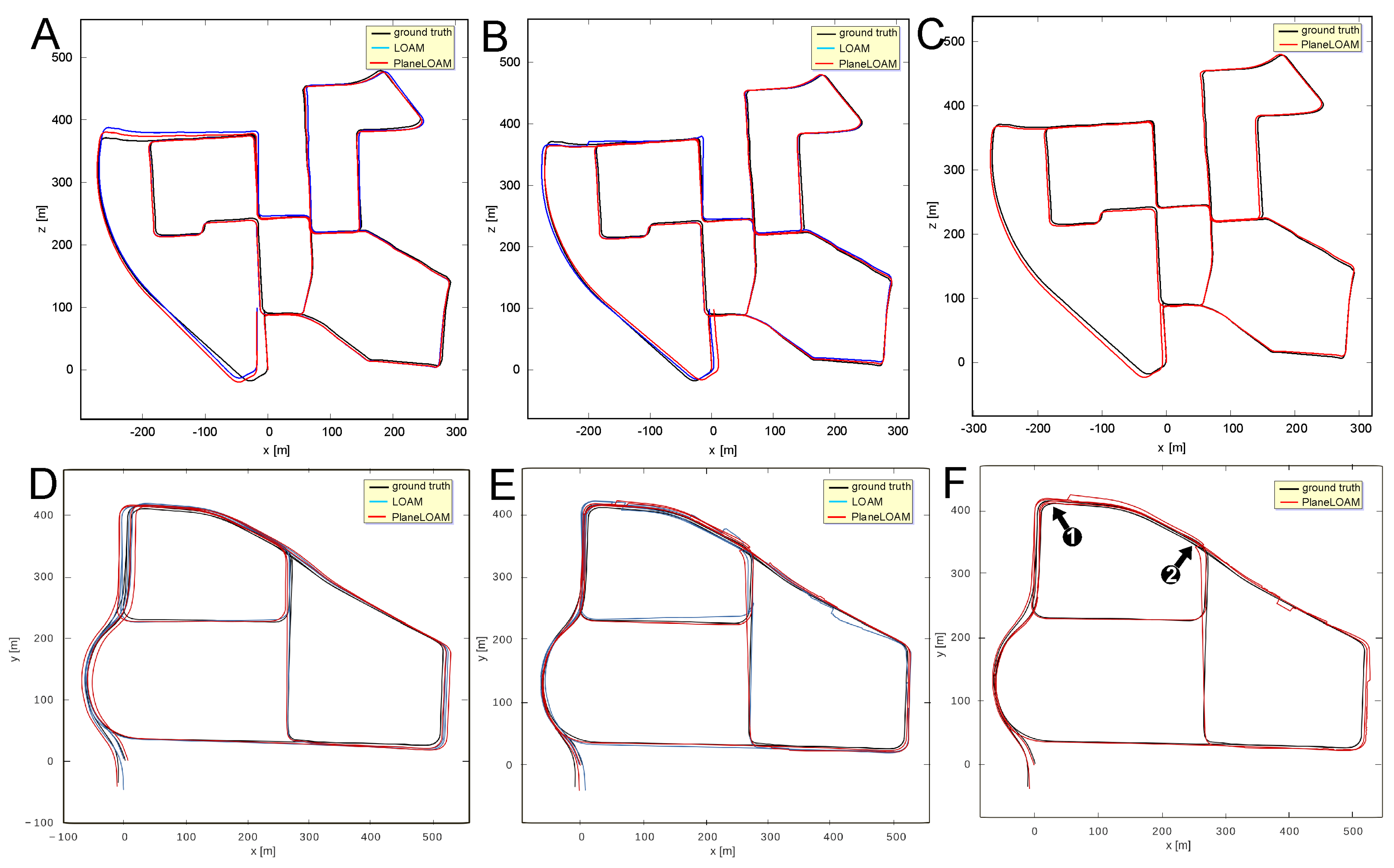
5.1. Accuracy of Trajectory Estimation with High-Level Features
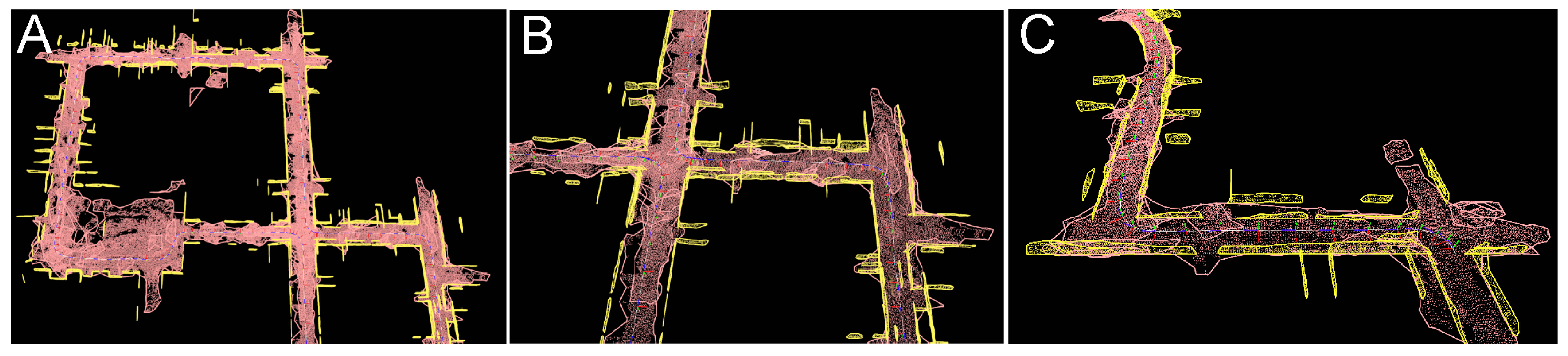
5.2. SLAM with High-Level Features in Different Environments
5.3. Analysis of the Computation Time
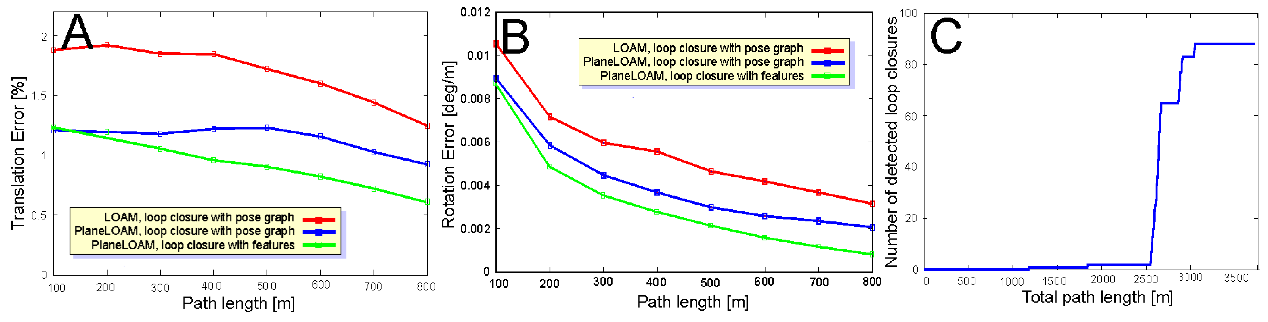
5.4. Different Approaches to Loop Closing in Feature-Based LiDAR SLAM
6. Conclusions
Author Contributions
Funding
Institutional Review Board Statement
Informed Consent Statement
Data Availability Statement
Conflicts of Interest
References
- Cadena, C.; Carlone, L.; Carrillo, H.; Latif, Y.; Scaramuzza, D.; Neira, J.; Reid, I.; Leonard, J.J. Past, Present, and Future of Simultaneous Localization And Mapping: Towards the Robust-Perception Age. IEEE Trans. Robot. 2016, 32, 1309–1332. [Google Scholar] [CrossRef]
- Bresson, G.; Alsayed, Z.; Yu, L.; Glaser, S. Simultaneous Localization And Mapping: A Survey of Current Trends in Autonomous Driving. IEEE Trans. Intell. Veh. 2017, 2, 194–220. [Google Scholar] [CrossRef]
- Li, Y.; Ibanez-Guzman, J. Lidar for autonomous driving: The principles, challenges, and trends for automotive lidar and perception systems. IEEE Signal Process. Mag. 2020, 37, 50–61. [Google Scholar] [CrossRef]
- Li, M.; Zhu, H.; You, S.; Tang, C.; Li, Y. Efficient Laser-Based 3D SLAM in Real Time for Coal Mine Rescue Robots. In Proceedings of the IEEE 8th Annual International Conference on CYBER Technology in Automation, Control, and Intelligent Systems, Tianjin, China, 19–23 July 2018; pp. 971–976. [Google Scholar]
- Mur-Artal, R.; Tardós, J.D. ORB-SLAM2: An open-source SLAM system for monocular, stereo and RGB-D cameras. IEEE Trans. Robot. 2017, 33, 1255–1262. [Google Scholar] [CrossRef]
- Hana, X.F.; Jin, J.; Xie, J.; Wang, M.J.; Jiang, W.A. Comprehensive Review of 3d Point Cloud Descriptors. arXiv 2018, arXiv:1802.02297. [Google Scholar]
- Triggs, B.; McLauchlan, P.; Hartley, R.; Fitzgibbon, A. Bundle adjustment—A modern synthesis. In Vision Algorithms: Theory and Practice, Lecture Notes in Computer Science; Triggs, B., Zisserman, S., Szeliski, R., Eds.; Springer: Cham, Switzerland, 2000; Volume 1883, pp. 298–372. [Google Scholar]
- Dubé, R.; Cramariuc, A.; Dugas, D.; Sommer, H.; Dymczyk, M.; Nieto, J.; Siegwart, R.; Cadena, C. SegMap: Segment-based mapping and localization using data-driven descriptors. Int. J. Robot. Res. 2020, 39, 339–355. [Google Scholar] [CrossRef]
- Zhang, J.; Singh, S. Low-drift and real-time LiDAR odometry and mapping. Auton. Robot. 2017, 41, 401–416. [Google Scholar] [CrossRef]
- Ćwian, K.; Nowicki, M.; Nowak, T.; Skrzypczyński, P. Planar Features for Accurate Laser-Based 3-D SLAM in Urban Environments. In Advanced, Contemporary Control; Bartoszewicz, A., Kabzinski, J., Kacprzyk, J., Eds.; AISC: Chicago, IL, USA, 2020; Volume 1196, pp. 941–953. [Google Scholar]
- Skrzypczyński, P. Mobile robot localization: Where we are and what are the challenges? In Automation 2017 Innovations in Automation, Robotics and Measurement Techniques; Springer: Cham, Switzerland, 2017; Volume 550, pp. 249–267. [Google Scholar]
- Campos, C.; Elvira, R.; Gómez Rodríguez, J.J.; Montiel, J.M.M.; Tardós, J.D. ORB-SLAM3: An accurate open-source library for visual, visual-inertial and multi-map SLAM. arXiv 2020, arXiv:2007.11898. [Google Scholar]
- Strasdat, H.; Montiel, J.; Davison, A. Real-time mococular SLAM: Why filter? In Proceedings of the IEEE International Conference on Robotics and Automation, Anchorage, AK, USA, 3–7 May 2010; pp. 2657–2664. [Google Scholar]
- Wulf, O.; Nüchter, A.; Hertzberg, J.; Wagner, B. Benchmarking urban six-degree-of-freedom simultaneous localization and mapping. J. Field Robot. 2008, 25, 148–163. [Google Scholar] [CrossRef]
- Bȩdkowski, J.; Röhling, T.; Hoeller, F.; Shulz, D.; Schneider, F. Benchmark of 6D SLAM (6D Simultaneous Localization and Mapping) algorithms with robotic mobile mapping systems. Found. Comput. Decis. Sci. 2017, 42, 275–295. [Google Scholar] [CrossRef]
- Moosmann, F.; Stiller, C. Velodyne SLAM. In Proceedings of the IEEE Intelligent Vehicles Symposium, Baden-Baden, Germany, 5–9 June 2011; pp. 393–398. [Google Scholar]
- Stoyanov, T.; Magnusson, M.; Andreasson, H.; Lilienthal, A.J. Fast and accurate scan registration through minimization of the distance between compact 3D NDT representations. Int. J. Robot. Res. 2012, 31, 1377–1393. [Google Scholar] [CrossRef]
- Whelan, T.; Leutenegger, S.; Moreno, R.S.; Glocker, B.; Davison, A. ElasticFusion: Dense SLAM Without A Pose Graph. In Proceedings of the Robotics: Science and Systems, Rome, Italy, 13–17 July 2015. [Google Scholar]
- Park, C.; Moghadam, P.; Kim, S.; Elfes, A.; Fookes, C.; Sridharan, S. Elastic LiDAR Fusion: Dense Map-Centric Continuous-Time SLAM. In Proceedings of the IEEE International Conference on Robotics and Automation (ICRA), Brisbane, Australia, 21–25 May 2018; pp. 1206–1213. [Google Scholar]
- Droeschel, D.; Behnke, S. Efficient Continuous-Time SLAM for 3D Lidar-Based Online Mapping. In Proceedings of the IEEE International Conference on Robotics and Automation, Brisbane, Australia, 21–25 May 2018; pp. 5000–5007. [Google Scholar]
- Behley, J.; Stachniss, C. Efficient surfel-based SLAM using 3D laser range data in urban environments. In Proceedings of the Robotics: Science and Systems, Pittsburgh, PA, USA, 26–30 June 2018. [Google Scholar]
- Liu, W.; Sun, J.; Li, W.; Hu, T.; Wang, P. Deep Learning on Point Clouds and Its Application: A Survey. Sensors 2019, 19, 4188. [Google Scholar] [CrossRef] [PubMed]
- Qi, C.; Su, H.; Mo, K.; Guibas, L.J. Pointnet: Deep learning on point sets for 3D classification and segmentation. In Proceedings of the IEEE Conference on Computer Vision and Pattern Recognition, Honolulu, HI, USA, 21–26 July 2017; pp. 652–660. [Google Scholar]
- Zhou, Y.; Tuzel, O. Voxelnet: End-to-end learning for point cloud based 3D object detection. In Proceedings of the IEEE/CVF Conference on Computer Vision and Pattern Recognition, Salt Lake City, UT, USA, 28–23 June 2018; pp. 4490–4499. [Google Scholar]
- Velas, M.; Spanel, M.; Hradis, M.; Herout, A. CNN for IMU assisted odometry estimation using Velodyne LiDAR. In Proceedings of the International Conference on Autnomous Robotic Systems and Computing, Vedras, Portugal, 25–27 April 2018; pp. 71–77. [Google Scholar]
- Lu, W.; Zhou, Y.; Wan, G.; Hou, S.; Song, S. L3-net: Towards Learning Based LiDAR Localization for Autonomous Driving. In Proceedings of the IEEE/CVF Conference on Computer Vision and Pattern Recognition (CVPR), Long Beach, CA, USA, 15–20 June 2019; pp. 6382–6391. [Google Scholar]
- Cho, Y.; Kim, G.; Kim, A. Unsupervised geometry-aware deep LiDAR odometry. In Proceedings of the IEEE International Conference on Robotics and Automation, Paris, France, 31 May–31 August 2020; pp. 2145–2152. [Google Scholar]
- Konolige, K. Sparse sparse bundle adjustment. In Proceedings of the British Machine Vision Conference, Aberystwyth, UK, 30 August–2 September 2010; pp. 102.1–102.11. [Google Scholar]
- Shan, T.; Englot, B. LeGO-LOAM: Lightweight and ground-optimized LiDAR odometry and mapping on variable terrain. In Proceedings of the IEEE/RSJ International Conferebce on Intelligent Robots and Systems, Madrid, Spain, 1–5 October 2018; pp. 4758–4765. [Google Scholar]
- Ji, X.; Zuo, L.; Zhang, C.; Liu, Y. LLOAM: LiDAR Odometry and Mapping with Loop-closure Detection Based Correction. In Proceedings of the IEEE International Conference on Mechatronics and Automation, Tianjin, China, 4–7 August 2019; pp. 2475–2480. [Google Scholar]
- Dubé, R.; Dugas, D.; Stumm, E.; Nieto, J.; Siegwart, R.; Cadena, C. SegMatch: Segment based place recognition in 3D point clouds. In Proceedings of the IEEE International Conference on Robotics and Automation, Singapore, 29 May–3 June 2017; pp. 5266–5272. [Google Scholar]
- Liu, X.; Zhang, L.; Qin, S.; Tian, D.; Ouyang, S.; Chen, C. Optimized LOAM Using Ground Plane Constraints and SegMatch-Based Loop Detection. Sensors 2019, 19, 5419. [Google Scholar] [CrossRef] [PubMed]
- Weingarten, J.; Siegwart, R. 3D SLAM using planar segments. In Proceedings of the IEEE/RSJ International Conference on Intelligent Robots and Systems, Beijing, China, 9–15 October 2006; pp. 3062–3067. [Google Scholar]
- Pathak, K.; Birk, A.; Vaskevicius, N.; Poppinga, J. Fast Registration Based on Noisy Planes with Unknown Correspondences for 3D Mapping. IEEE Trans. Robot. 2010, 26, 424–441. [Google Scholar] [CrossRef]
- Pathak, K.; Birk, A.; Vaskevicius, N.; Pfingsthorn, M.; Schwertfeger, S.; Poppinga, J. Online three-dimensional SLAM by registration of large planar surface segments and closed-form pose-graph relaxation. J. Field Robot. 2010, 27, 52–84. [Google Scholar] [CrossRef]
- Grant, W.S.; Voorhies, R.; Itti, L. Efficient Velodyne SLAM with point and plane features. Auton. Robot. 2019, 43, 1207–1224. [Google Scholar] [CrossRef]
- Pomerleau, F.; Colas, T.; Siegwart, R. A Review of Point Cloud Registration algorithms for mobile robotics. Found. Trends Robot. 2015, 4, 1–104. [Google Scholar] [CrossRef]
- Segal, A.; Haehnel, D.; Thrun, S. Generalized-ICP. In Proceedings of the Robotics: Science and Systems, Seattle, WA, USA, 28 June–1 July 2009. [Google Scholar]
- Deschaud, J. IMLS-SLAM: Scan-to-model matching based on 3D data. In Proceedings of the IEEE International Conference on Robotics and Automation, Brisbane, Australia, 21–25 May 2018; pp. 2480–2485. [Google Scholar]
- Elseberg, J.; Borrmann, D.; Lingemann, K.; Nüchter, A. Non-rigid registration and rectification of 3D laser scans. In Proceedings of the IEEE/RSJ International Conference on Intelligent Robots and Systems, Taipei, Taiwan, 18–22 October 2010; pp. 1546–1552. [Google Scholar]
- Neuhaus, F.; Koß, T.; Kohnen, R.; Paulus, D. MC2SLAM: Real-Time Inertial Lidar Odometry Using Two-Scan Motion Compensation. In Pattern Recognition; Brox, T., Bruhn, A., Fritz, M., Eds.; Springer International Publishing: Cham, Switzerland, 2019; pp. 60–72. [Google Scholar]
- Mendes, E.; Koch, P.; Lacroix, S. ICP-based pose-graph SLAM. In Proceedings of the IEEE International Symposium on Safety, Security, and Rescue Robotics, Lausanne, Switzerland, 23–27 October 2016; pp. 195–200. [Google Scholar]
- Magnusson, M.; Andreasson, H.; Nüchter, A.; Lilienthal, A.J. Appearance-based loop detection from 3D laser data using the normal distributions transform. In Proceedings of the IEEE International Conference on Robotics and Automation, Kobe, Japan, 12–17 May 2009; pp. 23–28. [Google Scholar]
- Buss, S.R.; Fillmore, J.P. Spherical averages and applications to spherical splines and interpolation. ACM Trans. Graph. 2001, 20, 95–126. [Google Scholar] [CrossRef]
- Bartoli, A. On the non-linear optimization of projective motion using minimal parameters. In European Conference on Computer Vision (ECCV); Springer: Berlin/Heidelberg, Germany, 2002; pp. 340–354. [Google Scholar]
- Sturm, J.; Engelhard, N.; Endres, F.; Burgard, W.; Cremers, D. A Benchmark for the Evaluation of RGB-D SLAM Systems. In Proceedings of the IEEE/RSJ International Conference on Intelligent Robots and Systems, Vilamoura-Algarve, Portugal, 7–12 October 2012. [Google Scholar]
- Umeyama, S. Least-squares estimation of transformation parameters between two point patterns. IEEE Trans. Pattern Anal. Mach. Intell. 1991, 13, 80–92. [Google Scholar] [CrossRef]
- Geiger, A.; Lenz, P.; Urtasun, R. Are we ready for Autonomous Driving? The KITTI Vision Benchmark Suite. In Proceedings of the Conference on Computer Vision and Pattern Recognition, Providence, RI, USA, 16–21 June 2012; pp. 3354–3361. [Google Scholar]
- Kim, G.; Park, Y.S.; Cho, Y.; Jeong, J.; Kim, A. MulRan: Multimodal Range Dataset for Urban Place Recognition. In Proceedings of the IEEE International Conference on Robotics and Automation, Paris, France, 31 May–31 August 2020; pp. 6246–6253. [Google Scholar]
- Nowak, T.; Ćwian, K.; Skrzypczyński, P. Cross-modal transfer learning for segmentation of non-stationary objects using LiDAR intensity data. In Proceedings of the IEEE International Conference on Robotics and Automation, Workshop on Sensing, Estimating and Understanding the Dynamic World, Paris, France, 31 May–31 August 2020. [Google Scholar]


| Dataset | PlaneLOAM | LOAM (Open-Source) | ||||
|---|---|---|---|---|---|---|
| Sequence | ||||||
| KITTI 00 | 4.52 m | 11.76 m | 2.36 m | 6.05 m | 11.55 m | 2.83 m |
| KITTI 05 | 3.21 m | 8.04 m | 1.59 m | 3.39 m | 11.26 m | 1.86 m |
| KITTI 07 | 0.50 m | 0.82 m | 0.20 m | 0.68 m | 1.28 m | 0.28 m |
| MulRan DCC | 11.02 m | 18.17 m | 4.46 m | 14.81 m | 27.95 m | 7.24 m |
| Dataset | PlaneLOAM | LOAM (Open-Source) | ||||
|---|---|---|---|---|---|---|
| Sequence | ||||||
| TownCentre | 4.93 m | 14.05 m | 2.10 m | 6.05 m | 24.90 m | 6.48 m |
| TownSuburbs | 4.91 m | 8.22 m | 1.79 m | 8.71 m | 18.37 m | 3.04 m |
| Posnania | 7.40 m | 17.50 m | 4.58 m | 15.90 m | 46.13 m | 9.99 m |
| Processing Step | Sub-Step | Computation Time [ms] | |||
|---|---|---|---|---|---|
| PlaneLOAM | LOAM (Open Source) | ||||
| Point clouds preparation | 8.18 | 7.70 | |||
| Construction of kd-tree | 2.49 | 75.80 | |||
| Point-to-line constraints | 14.05 | 18.77 | |||
| kd-tree search | 8.45 | 10.87 | |||
| other computations | 5.60 | 7.90 | |||
| Point-to-plane constraints | 13.11 | 18.30 | |||
| kd-tree search | 8.22 | 9.70 | |||
| other computations | 4.89 | 8.60 | |||
| Optimization time | 0.45 | 0.57 | |||
| Point clouds post-processing | 34.71 | 32.88 | |||
| Processing planar features | 35.77 | not applicable | |||
| adding points | 22.76 | ||||
| updating features | 2.22 | ||||
| deleting features | 0.02 | ||||
| merging features | 10.77 | ||||
| Processing linear features | 34.95 | not applicable | |||
| adding points | 15.53 | ||||
| updating features | 16.65 | ||||
| deleting features | 0.05 | ||||
| merging features | 2.72 | ||||
| Total time per scan | 143.71 | 154.02 | |||
| Approach to | PlaneLOAM | LOAM (Open Source) | ||||
|---|---|---|---|---|---|---|
| Loop Closing | ||||||
| none | 4.52 m | 11.76 m | 2.36 m | 6.05 m | 11.55 m | 2.83 m |
| pose graph | 3.96 m | 9.68 m | 2.17 m | 4.34 m | 11.15 m | 2.38 m |
| features alignment + BA | 2.47 m | 7.11 m | 1.48 m | N/A | N/A | N/A |
| Approach TO | PlaneLOAM | LOAM (Open-Source) | ||||
|---|---|---|---|---|---|---|
| Loop Closing | ||||||
| none | 11.02 m | 18.17 m | 4.46 m | 14.81 m | 27.95 m | 7.24 m |
| pose graph | 7.41 m | 19.23 m | 3.59 m | 9.77 m | 27.51 m | 4.26 m |
| features alignment + BA | 5.40 m | 13.78 m | 2.01 m | N/A | N/A | N/A |
Publisher’s Note: MDPI stays neutral with regard to jurisdictional claims in published maps and institutional affiliations. |
© 2021 by the authors. Licensee MDPI, Basel, Switzerland. This article is an open access article distributed under the terms and conditions of the Creative Commons Attribution (CC BY) license (https://creativecommons.org/licenses/by/4.0/).
Share and Cite
Ćwian, K.; Nowicki, M.R.; Wietrzykowski, J.; Skrzypczyński, P. Large-Scale LiDAR SLAM with Factor Graph Optimization on High-Level Geometric Features. Sensors 2021, 21, 3445. https://doi.org/10.3390/s21103445
Ćwian K, Nowicki MR, Wietrzykowski J, Skrzypczyński P. Large-Scale LiDAR SLAM with Factor Graph Optimization on High-Level Geometric Features. Sensors. 2021; 21(10):3445. https://doi.org/10.3390/s21103445
Chicago/Turabian StyleĆwian, Krzysztof, Michał R. Nowicki, Jan Wietrzykowski, and Piotr Skrzypczyński. 2021. "Large-Scale LiDAR SLAM with Factor Graph Optimization on High-Level Geometric Features" Sensors 21, no. 10: 3445. https://doi.org/10.3390/s21103445
APA StyleĆwian, K., Nowicki, M. R., Wietrzykowski, J., & Skrzypczyński, P. (2021). Large-Scale LiDAR SLAM with Factor Graph Optimization on High-Level Geometric Features. Sensors, 21(10), 3445. https://doi.org/10.3390/s21103445