
A Deep Learning Strategy for Automatic Sleep Staging Based on Two-Channel EEG Headband Data

 , , and
Abstract
1. Introduction
2. Materials and Methods
2.1. Data Collection
2.2. Data Preprocessing
2.2.1. Preprocessing PSG Data
2.2.2. Preprocessing HB Data
2.3. HB Data Cleaning
2.4. Data Augmentation
2.5. Deep Learning Model Architecture
2.6. Model Training
2.7. Traditional Sleep Staging Techniques
- Frequency domain;
- Time domain;
- Higher-order statistical analysis (HOSA)-based;
- Wavelet-based.
3. Results
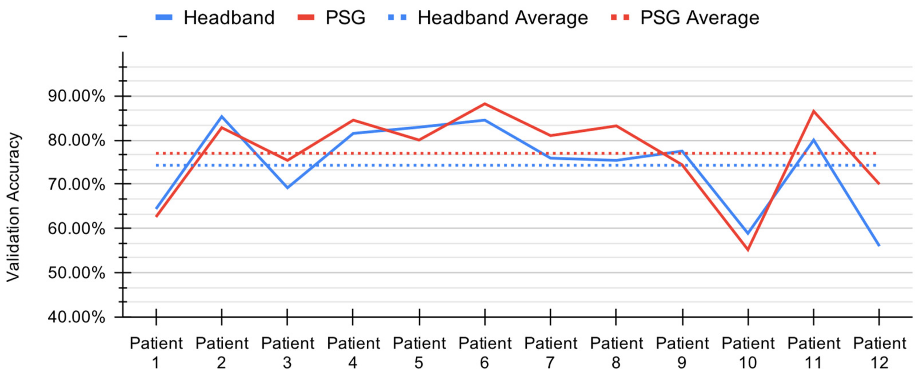
3.1. Deep Learning Model Performance
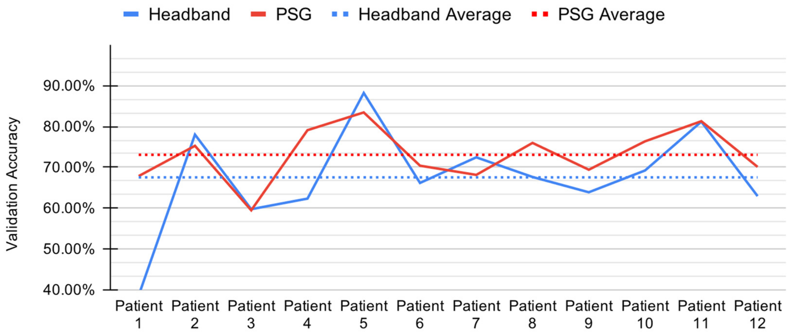
3.2. Baseline Model Performance
4. Discussion
4.1. Deep Learning Model Comparison
4.2. Baseline Model Comparison
4.3. Electrode Comparison
5. Conclusions
Author Contributions
Funding
Institutional Review Board Statement
Informed Consent Statement
Data Availability Statement
Acknowledgments
Conflicts of Interest
Appendix A

| Layer Type | Output Shape | Param # |
|---|---|---|
| Conv1D | (None, 2993, 8) | 136 |
| Activation (ReLU) | (None, 2993, 8) | 0 |
| MaxPooling1D | (None, 997, 8) | 0 |
| Conv1D | (None, 990, 16) | 1040 |
| Activation (ReLU) | (None, 990, 16) | 0 |
| MaxPooling1D | (None, 330, 16) | 0 |
| Conv1D | (None, 323, 32) | 4128 |
| Activation (ReLU) | (None, 323, 32) | 0 |
| MaxPooling1D | (None, 107, 32) | 0 |
| LSTM | (None, 107, 64) | 24,832 |
| LSTM | (None, 64) | 33,024 |
| Dense | (None, 5) | 325 |
| Total Params | 63,485 | |
| Trainable Params | 63,485 | |
| Non-Trainable Params | 0 |
| Headband (HB) | Polysomnography (PSG) | |
|---|---|---|
| Subject 1 |  |  |
| Subject 2 |  |  |
| Subject 3 |  |  |
| Subject 4 |  |  |
| Subject 5 |  |  |
| Subject 6 |  |  |
| Subject 7 |  |  |
| Subject 8 |  |  |
| Subject 9 |  |  |
| Subject 10 |  |  |
| Subject 11 |  |  |
| Subject 12 |  |  |
References
- Kent, B.A.; Feldman, H.H.; Nygaard, H.B. Sleep and Its Regulation: An Emerging Pathogenic and Treatment Frontier in Alzheimer’s Disease. Prog. Neurobiol. 2021, 197, 101902. [Google Scholar] [CrossRef] [PubMed]
- Arnal, P.J.; Thorey, V.; Ballard, M.E.; Hernandez, A.B.; Guillot, A.; Jourde, H.; Harris, M.; Guillard, M.; Beers, P.V.; Chennaoui, M.; et al. The Dreem Headband as an Alternative to Polysomnography for EEG Signal Acquisition and Sleep Staging. bioRxiv 2019, 662734. [Google Scholar] [CrossRef]
- Malkani, R.; Attarian, H. Sleep in Neurodegenerative Disorders. Curr. Sleep Med. Rep. 2015, 1, 81–90. [Google Scholar] [CrossRef][Green Version]
- Dora, C.; Biswal, P.K. An Improved Algorithm for Efficient Ocular Artifact Suppression from Frontal EEG Electrodes Using VMD. Biocybern. Biomed. Eng. 2020, 40, 148–161. [Google Scholar] [CrossRef]
- Lucey, B.P.; Mcleland, J.S.; Toedebusch, C.D.; Boyd, J.; Morris, J.C.; Landsness, E.C.; Yamada, K.; Holtzman, D.M. Comparison of a Single-Channel EEG Sleep Study to Polysomnography. J. Sleep Res. 2016, 25, 625–635. [Google Scholar] [CrossRef]
- Jackson, M.L.; Cavuoto, M.; Schembri, R.; Doré, V.; Villemagne, V.L.; Barnes, M.; O’Donoghue, F.J.; Rowe, C.C.; Robinson, S.R. Severe Obstructive Sleep Apnea Is Associated with Higher Brain Amyloid Burden: A Preliminary PET Imaging Study. J. Alzheimer’s Dis. 2020, 78, 611–617. [Google Scholar] [CrossRef]
- Santos-Mayo, L.; San-Jose-Revuelta, L.M.; Arribas, J.I. A Computer-Aided Diagnosis System With EEG Based on the P3b Wave During an Auditory Odd-Ball Task in Schizophrenia. IEEE Trans. Biomed. Eng. 2017, 64, 395–407. [Google Scholar] [CrossRef]
- Ashfaq Khan, M.; Kim, Y. Cardiac Arrhythmia Disease Classification Using LSTM Deep Learning Approach. Comput. Mater. Contin. 2021, 67, 427–443. [Google Scholar] [CrossRef]
- Giger, M.; Suzuki, K. Computer-Aided Diagnosis (CAD). In Biomedical Information Technology; Elsevier: Amsterdam, The Netherlands, 2007; pp. 359–374. ISBN 978-0-12-373583-6. [Google Scholar]
- Pineda, A.M.; Ramos, F.M.; Betting, L.E.; Campanharo, A.S.L.O. Quantile Graphs for EEG-Based Diagnosis of Alzheimer’s Disease. PLoS ONE 2020, 15, e0231169. [Google Scholar] [CrossRef]
- Hulbert, S.; Adeli, H. EEG/MEG- and Imaging-Based Diagnosis of Alzheimer’s Disease. Rev. Neurosci. 2013, 24, 563–576. [Google Scholar] [CrossRef]
- Roy, Y.; Banville, H.; Albuquerque, I.; Gramfort, A.; Falk, T.H.; Faubert, J. Deep Learning-Based Electroencephalography Analysis: A Systematic Review. J. Neural. Eng. 2019, 16, 051001. [Google Scholar] [CrossRef]
- Chambon, S.; Galtier, M.; Arnal, P.; Wainrib, G.; Gramfort, A. A Deep Learning Architecture for Temporal Sleep Stage Classification Using Multivariate and Multimodal Time Series. arXiv 2017, arXiv:1707.03321. [Google Scholar] [CrossRef]
- Neng, W.; Lu, J.; Xu, L. CCRRSleepNet: A Hybrid Relational Inductive Biases Network for Automatic Sleep Stage Classification on Raw Single-Channel EEG. Brain Sci. 2021, 11, 456. [Google Scholar] [CrossRef]
- Patanaik, A.; Ong, J.L.; Gooley, J.J.; Ancoli-Israel, S.; Chee, M.W.L. An End-to-End Framework for Real-Time Automatic Sleep Stage Classification. Sleep 2018, 41. [Google Scholar] [CrossRef]
- Ismail Fawaz, H.; Forestier, G.; Weber, J.; Idoumghar, L.; Muller, P.-A. Deep Learning for Time Series Classification: A Review. Data Min. Knowl. Disc. 2019, 33, 917–963. [Google Scholar] [CrossRef]
- Bickel, S.; Brückner, M.; Scheffer, T. Discriminative Learning under Covariate Shift. J. Mach. Learn. Res. 2019, 10, 2137–2155. [Google Scholar]
- AWS S3 Explorer. Available online: https://dreem-octave-irba.s3.eu-west-3.amazonaws.com/index.html (accessed on 24 March 2021).
- Griessenberger, H.; Heib, D.P.J.; Kunz, A.B.; Hoedlmoser, K.; Schabus, M. Assessment of a Wireless Headband for Automatic Sleep Scoring. Sleep Breath 2013, 17, 747–752. [Google Scholar] [CrossRef]
- Zhang, Z.; Guan, C. An Accurate Sleep Staging System with Novel Feature Generation and Auto-Mapping. In Proceedings of the 2017 International Conference on Orange Technologies (ICOT), Singapore, 8–10 December 2017; pp. 214–217. [Google Scholar]
- Dong, H.; Supratak, A.; Pan, W.; Wu, C.; Matthews, P.M.; Guo, Y. Mixed Neural Network Approach for Temporal Sleep Stage Classification. IEEE Trans. Neural. Syst. Rehabil. Eng. 2018, 26, 324–333. [Google Scholar] [CrossRef]
- Levendowski, D.J.; Ferini-Strambi, L.; Gamaldo, C.; Cetel, M.; Rosenberg, R.; Westbrook, P.R. The Accuracy, Night-to-Night Variability, and Stability of Frontopolar Sleep Electroencephalography Biomarkers. J. Clin. Sleep Med. 2017, 13, 791–803. [Google Scholar] [CrossRef]
- Berry, R.B.; Brooks, R.; Gamaldo, C.; Harding, S.M.; Lloyd, R.M.; Quan, S.F.; Troester, M.T.; Vaughn, B.V. AASM Scoring Manual Updates for 2017 (Version 2.4). J. Clin. Sleep Med. 2017, 13, 665–666. [Google Scholar] [CrossRef]
- Dry EEG Headset | CGX | United States. Available online: https://www.cgxsystems.com/ (accessed on 27 April 2021).
- Patel, A.K.; Reddy, V.; Araujo, J.F. Physiology, Sleep Stages. In StatPearls; StatPearls Publishing: Treasure Island, FL, USA, 2021. [Google Scholar]
- Aurlien, H.; Gjerde, I.O.; Aarseth, J.H.; Eldøen, G.; Karlsen, B.; Skeidsvoll, H.; Gilhus, N.E. EEG Background Activity Described by a Large Computerized Database. Clin. Neurophysiol. 2004, 115, 665–673. [Google Scholar] [CrossRef]
- Shukla, A.; Majumdar, A. Exploiting Inter-Channel Correlation in EEG Signal Reconstruction. Biomed. Signal Process. Control 2015, 18, 49–55. [Google Scholar] [CrossRef]
- Lashgari, E.; Liang, D.; Maoz, U. Data Augmentation for Deep-Learning-Based Electroencephalography. J. Neurosci. Methods 2020, 346, 108885. [Google Scholar] [CrossRef]
- O’Shea, A.; Lightbody, G.; Boylan, G.; Temko, A. Neonatal Seizure Detection Using Convolutional Neural Networks. In Proceedings of the 2017 IEEE 27th International Workshop on Machine Learning for Signal Processing (MLSP), Tokyo, Japan, 25–28 September 2017; pp. 1–6. [Google Scholar]
- Majidov, I.; Whangbo, T. Efficient Classification of Motor Imagery Electroencephalography Signals Using Deep Learning Methods. Sensors 2019, 19, 1736. [Google Scholar] [CrossRef]
- Ullah, I.; Hussain, M.; Qazi, E.-H.; Aboalsamh, H. An Automated System for Epilepsy Detection Using EEG Brain Signals Based on Deep Learning Approach. Expert Syst. Appl. 2018, 107, 61–71. [Google Scholar] [CrossRef]
- Sors, A.; Bonnet, S.; Mirek, S.; Vercueil, L.; Payen, J.-F. A Convolutional Neural Network for Sleep Stage Scoring from Raw Single-Channel EEG. Biomed. Signal Process. Control 2018, 42, 107–114. [Google Scholar] [CrossRef]
- Tsinalis, O.; Matthews, P.M.; Guo, Y.; Zafeiriou, S. Automatic Sleep Stage Scoring with Single-Channel EEG Using Convolutional Neural Networks. arXiv 2016, arXiv:1610.01683. [Google Scholar]
- Vilamala, A.; Madsen, K.H.; Hansen, L.K. Deep Convolutional Neural Networks for Interpretable Analysis of EEG Sleep Stage Scoring. arXiv 2017, arXiv:1710.00633. [Google Scholar]
- Xu, Z.; Yang, X.; Sun, J.; Liu, P.; Qin, W. Sleep Stage Classification Using Time-Frequency Spectra From Consecutive Multi-Time Points. Front. Neurosci. 2020, 14. [Google Scholar] [CrossRef] [PubMed]
- Supratak, A.; Dong, H.; Wu, C.; Guo, Y. DeepSleepNet: A Model for Automatic Sleep Stage Scoring Based on Raw Single-Channel EEG. IEEE Trans. Neural. Syst. Rehabil. Eng. 2017, 25, 1998–2008. [Google Scholar] [CrossRef] [PubMed]
- Bresch, E.; Großekathöfer, U.; Garcia-Molina, G. Recurrent Deep Neural Networks for Real-Time Sleep Stage Classification From Single Channel EEG. Front. Comput. Neurosci. 2018, 12. [Google Scholar] [CrossRef]
- Xie, L.; Wang, J.; Wei, Z.; Wang, M.; Tian, Q. DisturbLabel: Regularizing CNN on the Loss Layer. In Proceedings of the 2016 Institute of Electrical and Electronics Engineers (IEEE) Conference on Computer Vision and Pattern Recognition, Las Vegas, NV, USA, 27–30 June 2016; pp. 4753–4762. [Google Scholar]
- Zheng, Q.; Yang, M.; Tian, X.; Jiang, N.; Wang, D. A Full Stage Data Augmentation Method in Deep Convolutional Neural Network for Natural Image Classification. Discret. Dyn. Nat. Soc. 2020, 2020, e4706576. [Google Scholar] [CrossRef]
- Srivastava, N.; Hinton, G.; Krizhevsky, A.; Sutskever, I.; Salakhutdinov, R. Dropout: A Simple Way to Prevent Neural Networks from Overfitting. J. Mach. Learn. Res. 2014, 15, 1929–1958. [Google Scholar]
- Kingma, D.P.; Ba, J. Adam: A Method for Stochastic Optimization. arXiv 2017, arXiv:1412.6980. [Google Scholar]
- Rosenberg, R.S.; Van Hout, S. The American Academy of Sleep Medicine Inter-Scorer Reliability Program: Sleep Stage Scoring. J. Clin. Sleep Med. 2013, 09, 81–87. [Google Scholar] [CrossRef]
- Fiorillo, L.; Puiatti, A.; Papandrea, M.; Ratti, P.-L.; Favaro, P.; Roth, C.; Bargiotas, P.; Bassetti, C.L.; Faraci, F.D. Automated Sleep Scoring: A Review of the Latest Approaches. Sleep Med. Rev. 2019, 48, 101204. [Google Scholar] [CrossRef]
- Mathewson, K.E.; Harrison, T.J.L.; Kizuk, S.A.D. High and Dry? Comparing Active Dry EEG Electrodes to Active and Passive Wet Electrodes. Psychophysiology 2017, 54, 74–82. [Google Scholar] [CrossRef]
- Li, G.-L.; Wu, J.-T.; Xia, Y.-H.; He, Q.-G.; Jin, H.-G. Review of Semi-Dry Electrodes for EEG Recording. J. Neural Eng. 2020, 17, 051004. [Google Scholar] [CrossRef]
- Li, G.; Wu, J.; Xia, Y.; Wu, Y.; Tian, Y.; Liu, J.; Chen, D.; He, Q. Towards Emerging EEG Applications: A Novel Printable Flexible Ag/AgCl Dry Electrode Array for Robust Recording of EEG Signals at Forehead Sites. J. Neural Eng. 2020, 17, 026001. [Google Scholar] [CrossRef]
- Li, G.; Wang, S.; Li, M.; Duan, Y.Y. Towards Real-Life EEG Applications: Novel Superporous Hydrogel-Based Semi-Dry EEG Electrodes Enabling Automatically ‘charge–Discharge’ Electrolyte. J. Neural Eng. 2021, 18, 046016. [Google Scholar] [CrossRef]


| Bandwidth | Sample Rate | Amplifier Gain | Resolution | Noise |
|---|---|---|---|---|
| 0–131 Hz | 500 samples/sec | 6 | 24 bits/sample | 0.7 μV |
| Feature Category | Feature Group | Feature Size |
|---|---|---|
| Frequency Domain | RSP | 11 |
| HP | 15 | |
| SWI | 3 | |
| Time Domain | Hjorth | 3 |
| Skewness | 1 | |
| Kurtosis | 1 | |
| HOSA | Bi-Spectrum | 20 |
| Wavelet | Relative Power | 8 |
| Total Features | 62 |
| Data | N1 | N2 | N3 | REM | Wake | Accuracy | Balanced Accuracy |
|---|---|---|---|---|---|---|---|
| HB | 29.80% | 74.87% | 84.02% | 73.96% | 80.60% | 74.01% | 68.65% |
| PSG | 31.08% | 77.82% | 85.27% | 75.38% | 84.64% | 77.00% | 70.84% |
| Data | N1 | N2 | N3 | REM | Wake | Accuracy | Balanced Accuracy |
|---|---|---|---|---|---|---|---|
| HB | 4.11% | 82.32% | 49.65% | 28.26% | 80.03% | 67.53% | 48.88% |
| PSG | 13.13% | 88.36% | 35.90% | 55.17% | 83.49% | 73.06% | 55.21% |
Publisher’s Note: MDPI stays neutral with regard to jurisdictional claims in published maps and institutional affiliations. |
© 2021 by the authors. Licensee MDPI, Basel, Switzerland. This article is an open access article distributed under the terms and conditions of the Creative Commons Attribution (CC BY) license (https://creativecommons.org/licenses/by/4.0/).
Share and Cite
Casciola, A.A.; Carlucci, S.K.; Kent, B.A.; Punch, A.M.; Muszynski, M.A.; Zhou, D.; Kazemi, A.; Mirian, M.S.; Valerio, J.; McKeown, M.J.; et al. A Deep Learning Strategy for Automatic Sleep Staging Based on Two-Channel EEG Headband Data. Sensors 2021, 21, 3316. https://doi.org/10.3390/s21103316
Casciola AA, Carlucci SK, Kent BA, Punch AM, Muszynski MA, Zhou D, Kazemi A, Mirian MS, Valerio J, McKeown MJ, et al. A Deep Learning Strategy for Automatic Sleep Staging Based on Two-Channel EEG Headband Data. Sensors. 2021; 21(10):3316. https://doi.org/10.3390/s21103316
Chicago/Turabian StyleCasciola, Amelia A., Sebastiano K. Carlucci, Brianne A. Kent, Amanda M. Punch, Michael A. Muszynski, Daniel Zhou, Alireza Kazemi, Maryam S. Mirian, Jason Valerio, Martin J. McKeown, and et al. 2021. "A Deep Learning Strategy for Automatic Sleep Staging Based on Two-Channel EEG Headband Data" Sensors 21, no. 10: 3316. https://doi.org/10.3390/s21103316
APA StyleCasciola, A. A., Carlucci, S. K., Kent, B. A., Punch, A. M., Muszynski, M. A., Zhou, D., Kazemi, A., Mirian, M. S., Valerio, J., McKeown, M. J., & Nygaard, H. B. (2021). A Deep Learning Strategy for Automatic Sleep Staging Based on Two-Channel EEG Headband Data. Sensors, 21(10), 3316. https://doi.org/10.3390/s21103316