Active and Passive Electro-Optical Sensors for Health Assessment in Food Crops


 ,
,  ,
,
Abstract
1. Introduction
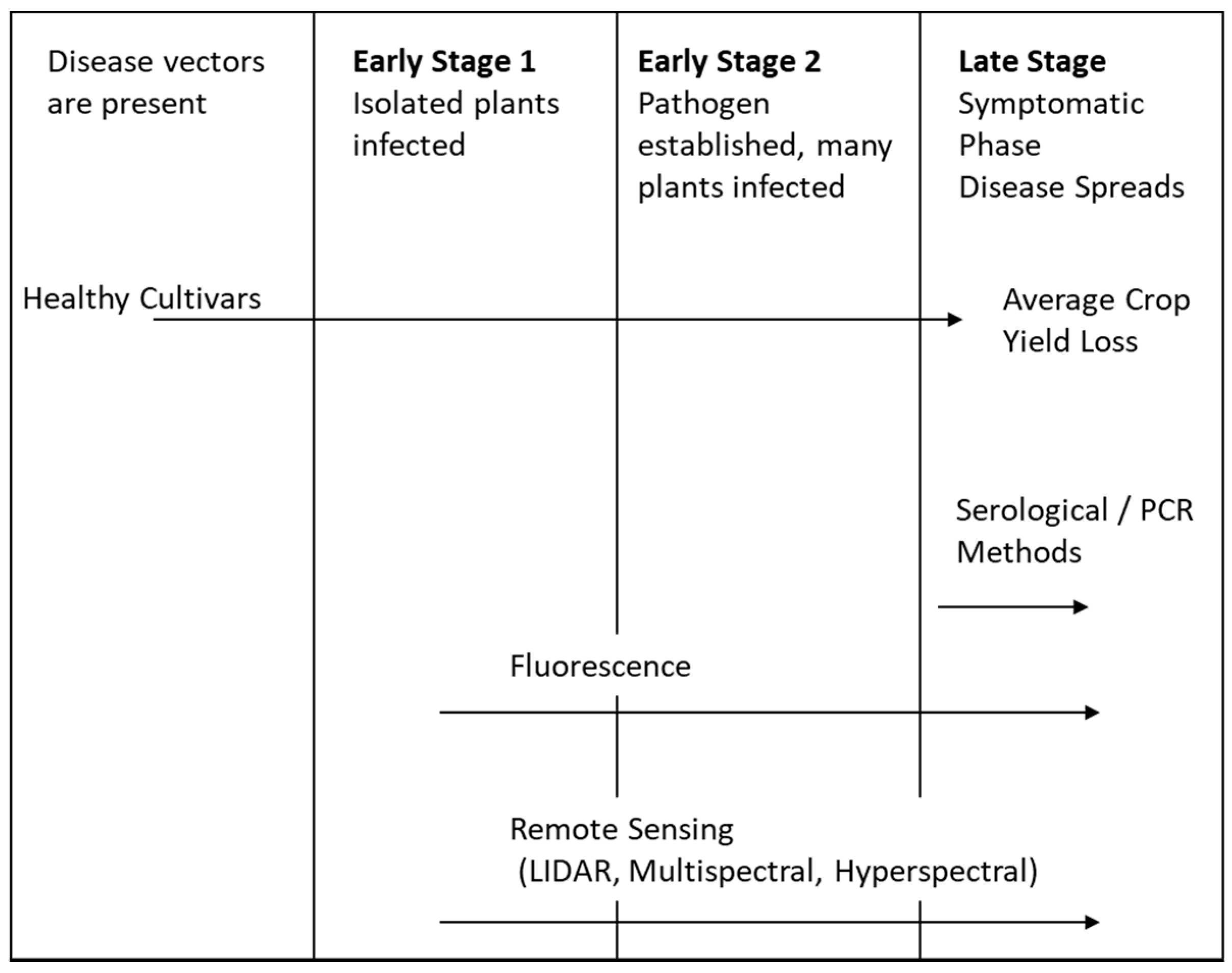
2. Background
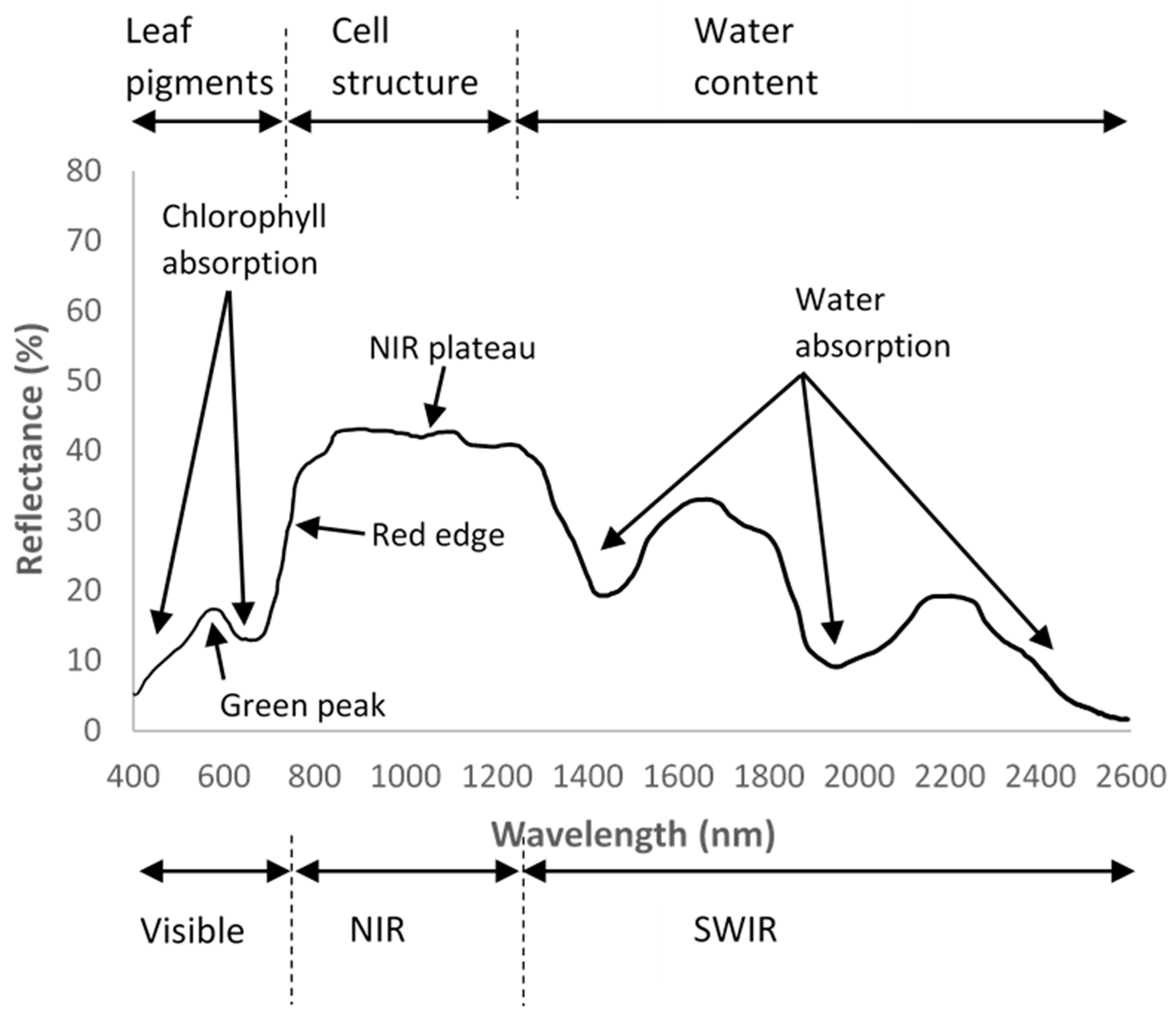
2.1. Plant Biology in Relation to Sensors
2.2. Wavelength Bands
2.3. Plant Breeding
2.4. Soil Monitoring
2.5. Classification Indices
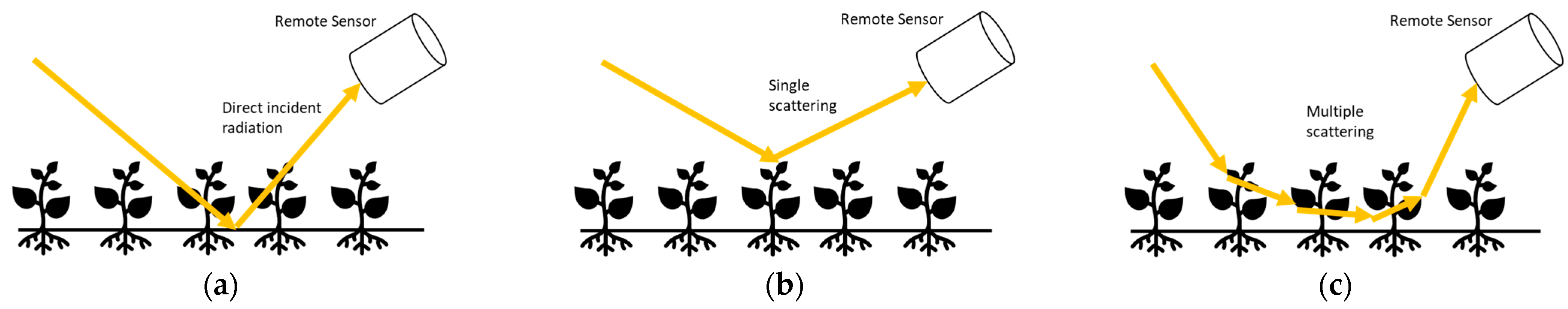
2.6. Bidirectional Reflectance Distribution Function Measurement
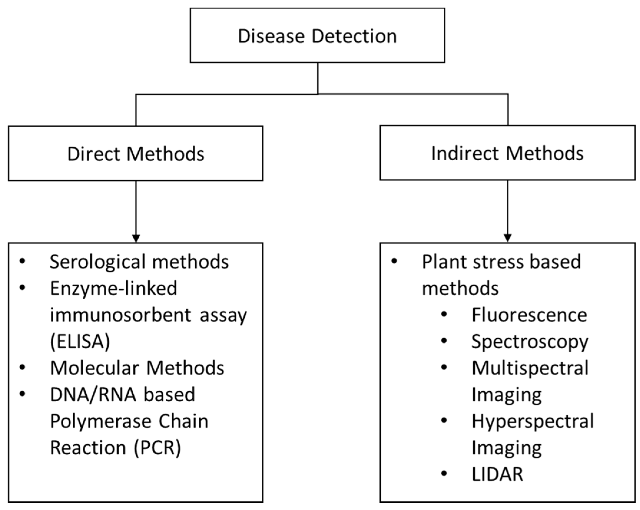
3. Proximal Sensors
3.1. Traditional Molecular Methods
3.1.1. Serological Assays
3.1.2. Nucleic Acid-Based Methods
3.2. Fluorescence Spectroscopy
4. Remote Sensing
4.1. Multispectral Imaging
4.2. Hyperspectral Imaging
4.3. Thermography
4.4. LIDAR
Carbon Dioxide Absorption Spectroscopy
4.5. LIDAR Shape Profiling and 3D Scanners
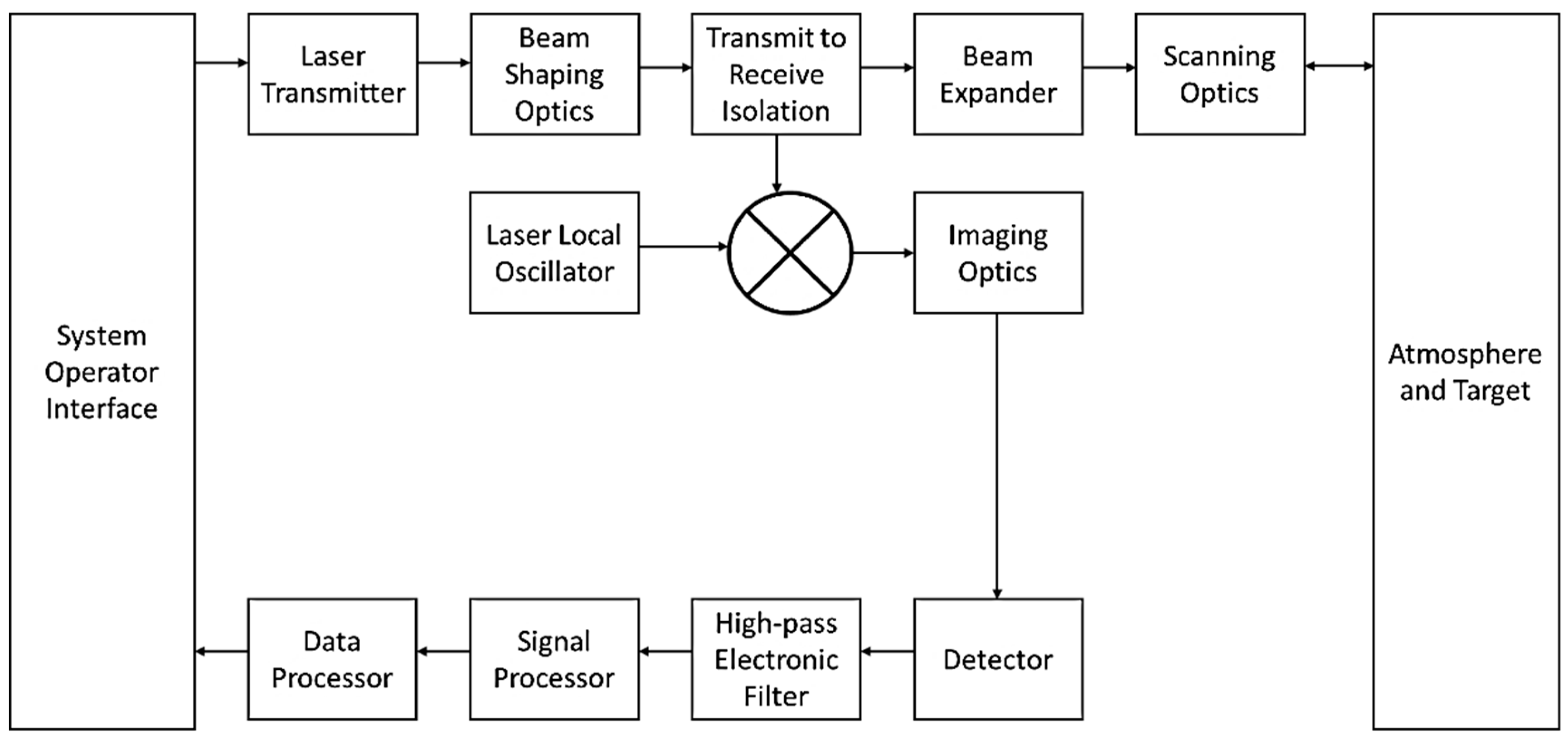
4.6. Bistatic LIDAR System Concept
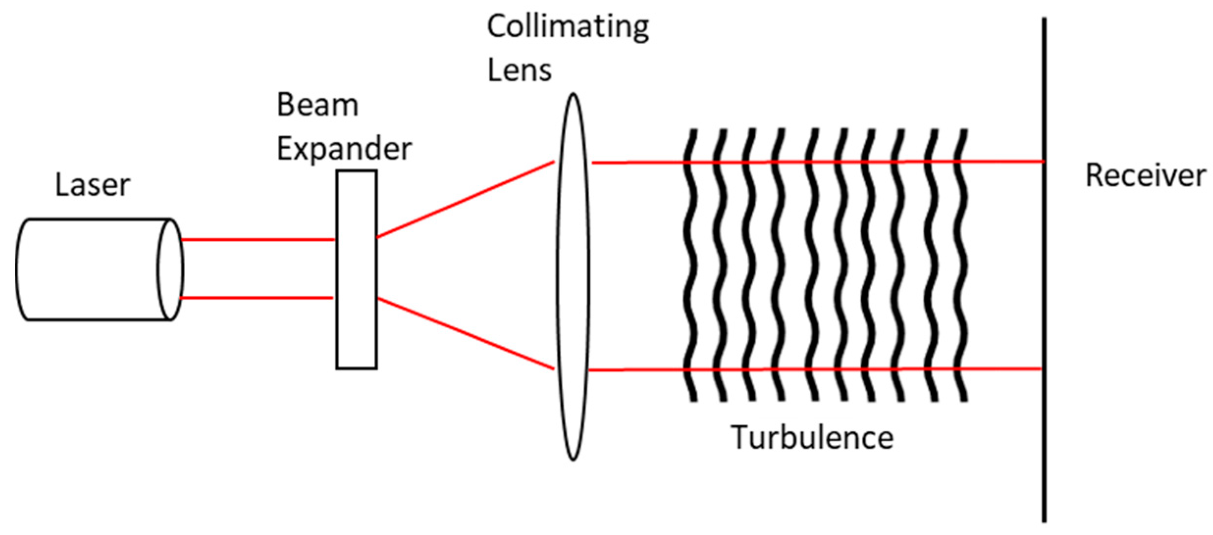
LIDAR Laser Beam Propagation in the Atmosphere
4.7. Hyperspectral and LIDAR RS Fusion
5. Food Quality Analysis
5.1. Fluorescence Spectroscopy
5.2. Multispectral Imaging
5.3. Hyperspectral Imaging
5.4. LIDAR
6. Remote Sensor Platforms
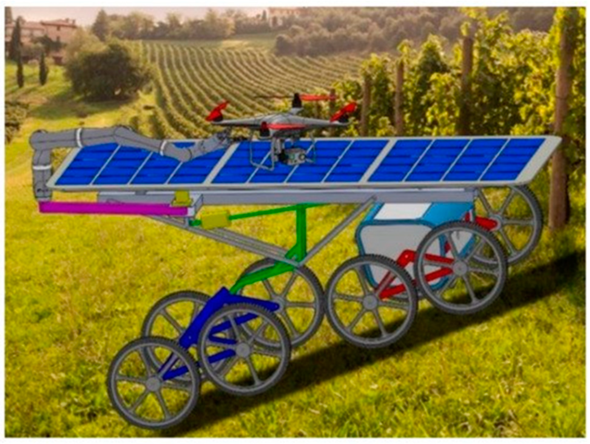
UGV and UAV Cooperative Approaches
7. Data Analysis Methods
7.1. Partial Least Squares Regression
7.2. Principal Component Analysis
7.3. Self-Organizing Maps
7.4. Artificial Neural Networks
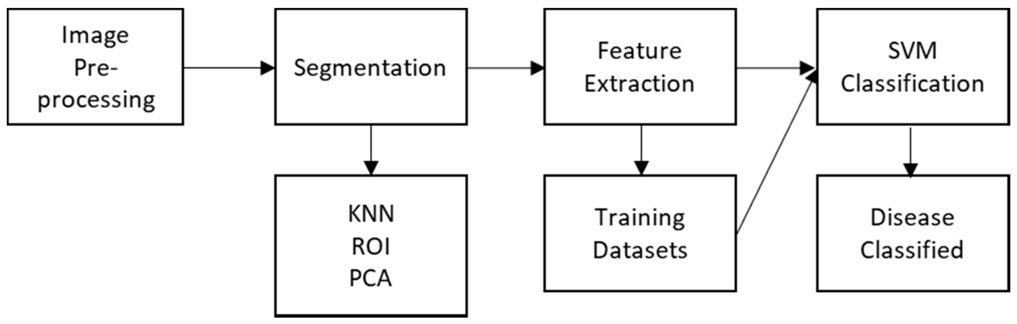
7.5. Support Vector Machines
7.6. K-Nearest Neighbours
7.7. Regions of Interest
8. Conclusions
Author Contributions
Funding
Conflicts of Interest
References
- Martinelli, F.; Scalenghe, R.; Davino, S.; Panno, S.; Scuderi, G.; Ruisi, P.; Villa, P.; Stroppiana, D.; Boschetti, M.; Goulart, L.R. Advanced methods of plant disease detection. A review. Agron. Sustain. Dev. 2015, 35, 1–25. [Google Scholar] [CrossRef]
- Christou, P.; Twyman, R.M. The potential of genetically enhanced plants to address food insecurity. Nutr. Res. Rev. 2004, 17, 23–42. [Google Scholar] [CrossRef] [PubMed]
- Strange, R.N.; Scott, P.R. Plant disease: A threat to global food security. Annu. Rev. Phytopathol. 2005, 43, 83–116. [Google Scholar] [CrossRef] [PubMed]
- Steffen, W.; Sims, J.; Walcott, J.; Laughlin, G. Australian agriculture: Coping with dangerous climate change. Reg. Environ. Chang. 2011, 11, 205–214. [Google Scholar] [CrossRef]
- Huang, W.; Luo, J.; Zhang, J.; Zhao, J.; Zhao, C.; Wang, J.; Yang, G.; Huang, M.; Huang, L.; Du, S. Crop disease and pest monitoring by remote sensing. In Remote Sensing-Applications; IntechOpen: Rijeka, Croatia, 2012. [Google Scholar]
- De Jong, S.M.; Van der Meer, F.D. Remote Sensing Image Analysis: Including the Spatial domain; Springer Science & Business Media: New York, NY, USA, 2007; Volume 5. [Google Scholar]
- Atkinson, N.J.; Urwin, P.E. The interaction of plant biotic and abiotic stresses: From genes to the field. J. Exp. Bot. 2012, 63, 3523–3543. [Google Scholar] [CrossRef]
- Rumpf, T.; Mahlein, A.-K.; Steiner, U.; Oerke, E.-C.; Dehne, H.-W.; Plümer, L. Early detection and classification of plant diseases with support vector machines based on hyperspectral reflectance. Comput. Electron. Agric. 2010, 74, 91–99. [Google Scholar] [CrossRef]
- Nutter, F.W.; van Rij, N.; Eggenberger, S.K.; Holah, N. Spatial and temporal dynamics of plant pathogens. In Precision Crop Protection-the Challenge and Use of Heterogeneity; Springer: Berlin/Heidelberg, Germany, 2010; pp. 27–50. [Google Scholar]
- Stafford, J.V. Implementing precision agriculture in the 21st century. J. Agric. Eng. Res. 2000, 76, 267–275. [Google Scholar] [CrossRef]
- Mahlein, A.-K.; Oerke, E.-C.; Steiner, U.; Dehne, H.-W. Recent advances in sensing plant diseases for precision crop protection. Eur. J. Plant Pathol. 2012, 133, 197–209. [Google Scholar] [CrossRef]
- Maxwell, K.; Johnson, G.N. Chlorophyll fluorescence—A practical guide. J. Exp. Bot. 2000, 51, 659–668. [Google Scholar] [CrossRef]
- Lee, W.-S.; Alchanatis, V.; Yang, C.; Hirafuji, M.; Moshou, D.; Li, C. Sensing technologies for precision specialty crop production. Comput. Electron. Agric. 2010, 74, 2–33. [Google Scholar] [CrossRef]
- Jacquemoud, S.; Ustin, S.L. Leaf optical properties: A state of the art. In Proceedings of the 8th International Symposium of Physical Measurements & Signatures in Remote Sensing, Aussois, France, 8–12 January 2001; pp. 223–332. [Google Scholar]
- Mouazen, A.M.; Alexandridis, T.; Buddenbaum, H.; Cohen, Y.; Moshou, D.; Mulla, D.; Nawar, S.; Sudduth, K.A. Monitoring. In Agricultural Internet of Things and Decision Support for Precision Smart Farming; Elsevier: Amsterdam, The Netherlands, 2020; pp. 35–138. [Google Scholar]
- Teke, M.; Deveci, H.S.; Haliloğlu, O.; Gürbüz, S.Z.; Sakarya, U. A short survey of hyperspectral remote sensing applications in agriculture. In Proceedings of the 2013 6th International Conference on Recent Advances in Space Technologies (RAST), Istanbul, Turkey, 12–14 June 2013; pp. 171–176. [Google Scholar]
- Sahoo, R.N.; Ray, S.; Manjunath, K. Hyperspectral remote sensing of agriculture. Curr. Sci. 2015, 108, 848–859. [Google Scholar]
- Jorge, L.A.; Brandão, Z.; Inamasu, R. Insights and Recommendations of Use of UAV Platforms in Precision Agriculture in Brazil; SPIE: Bellingham, WA, USA, 2014; Volume 9239. [Google Scholar]
- Ustin, S.L.; Gamon, J.A. Remote sensing of plant functional types. New Phytol. 2010, 186, 795–816. [Google Scholar] [CrossRef] [PubMed]
- Varshney, P.K.; Arora, M.K. Advanced Image Processing Techniques for Remotely Sensed Hyperspectral Data; Springer Science & Business Media: New York, NY, USA, 2004. [Google Scholar]
- Shimelis, H.; Laing, M. Timelines in conventional crop improvement: Pre-breeding and breeding procedures. Aust. J. Crop Sci. 2012, 6, 1542. [Google Scholar]
- Kuska, M.; Wahabzada, M.; Leucker, M.; Dehne, H.-W.; Kersting, K.; Oerke, E.-C.; Steiner, U.; Mahlein, A.-K. Hyperspectral phenotyping on the microscopic scale: Towards automated characterization of plant-pathogen interactions. Plant Methods 2015, 11, 28. [Google Scholar] [CrossRef] [PubMed]
- Rascher, U.; Blossfeld, S.; Fiorani, F.; Jahnke, S.; Jansen, M.; Kuhn, A.J.; Matsubara, S.; Märtin, L.L.; Merchant, A.; Metzner, R. Non-invasive approaches for phenotyping of enhanced performance traits in bean. Funct. Plant Biol. 2011, 38, 968–983. [Google Scholar] [CrossRef] [PubMed]
- Magalhães, A.; Kubota, T.; Boas, P.; Meyer, M.; Milori, D. Non-destructive fluorescence spectroscopy as a phenotyping technique in soybeans. In Proceedings of the II Latin-American Conference on Plant Phenotyping and Phenomics for Plant Breeding, São Carlos, Brazil, 20–22 September 2017. [Google Scholar]
- Romano, G.; Zia, S.; Spreer, W.; Sanchez, C.; Cairns, J.; Araus, J.L.; Müller, J. Use of thermography for high throughput phenotyping of tropical maize adaptation in water stress. Comput. Electron. Agric. 2011, 79, 67–74. [Google Scholar] [CrossRef]
- Guo, Q.; Wu, F.; Pang, S.; Zhao, X.; Chen, L.; Liu, J.; Xue, B.; Xu, G.; Li, L.; Jing, H. Crop 3D—A LiDAR based platform for 3D high-throughput crop phenotyping. Sci. China Life Sci. 2018, 61, 328–339. [Google Scholar] [CrossRef]
- Bi, K.; Xiao, S.; Gao, S.; Zhang, C.; Huang, N.; Niu, Z. Estimating Vertical Chlorophyll Concentrations in Maize in Different Health States Using Hyperspectral LiDAR. IEEE Trans. Geosci. Remote Sens. 2020, 58, 8125–8133. [Google Scholar] [CrossRef]
- Walter, J.D.C.; Edwards, J.; McDonald, G.; Kuchel, H. Estimating biomass and canopy height with lidar for field crop breeding. Front. Plant Sci. 2019, 10, 1145. [Google Scholar] [CrossRef]
- Lin, Y. LiDAR: An important tool for next-generation phenotyping technology of high potential for plant phenomics? Comput. Electron. Agric. 2015, 119, 61–73. [Google Scholar] [CrossRef]
- Bajcsy, P.; Groves, P. Methodology for hyperspectral band selection. Photogramm. Eng. Remote Sens. 2004, 70, 793–802. [Google Scholar] [CrossRef]
- Pinter, P.J., Jr.; Hatfield, J.L.; Schepers, J.S.; Barnes, E.M.; Moran, M.S.; Daughtry, C.S.; Upchurch, D.R. Remote sensing for crop management. Photogramm. Eng. Remote Sens. 2003, 69, 647–664. [Google Scholar] [CrossRef]
- Liu, K.; Zhou, Q.-B.; Wu, W.-B.; Xia, T.; Tang, H.-J. Estimating the crop leaf area index using hyperspectral remote sensing. J. Integr. Agric. 2016, 15, 475–491. [Google Scholar] [CrossRef]
- Hu, J.; Peng, J.; Zhou, Y.; Xu, D.; Zhao, R.; Jiang, Q.; Fu, T.; Wang, F.; Shi, Z. Quantitative estimation of soil salinity using UAV-borne hyperspectral and satellite multispectral images. Remote Sens. 2019, 11, 736. [Google Scholar] [CrossRef]
- Ge, X.; Wang, J.; Ding, J.; Cao, X.; Zhang, Z.; Liu, J.; Li, X. Combining UAV-based hyperspectral imagery and machine learning algorithms for soil moisture content monitoring. PeerJ 2019, 7, e6926. [Google Scholar] [CrossRef] [PubMed]
- Tilman, D.; Cassman, K.G.; Matson, P.A.; Naylor, R.; Polasky, S. Agricultural sustainability and intensive production practices. Nature 2002, 418, 671–677. [Google Scholar] [CrossRef]
- Pérez, E.; García, P. Monitoring soil erosion by raster images: From aerial photographs to drone taken pictures. Eur. J. Geogr. 2017, 7, 117–129. [Google Scholar]
- Thenkabail, P.S.; Gumma, M.K.; Teluguntla, P.; Mohammed, I.A. Hyperspectral remote sensing of vegetation and agricultural crops. Photogramm. Eng. Remote Sens. 2014, 80, 697–723. [Google Scholar]
- Myneni, R.B.; Ross, J. Photon-Vegetation Interactions: Applications in Optical Remote Sensing and Plant Ecology; Springer Science & Business Media: New York, NY, USA, 2012. [Google Scholar]
- Qi, J.; Kerr, Y.; Moran, M.; Weltz, M.; Huete, A.; Sorooshian, S.; Bryant, R. Leaf area index estimates using remotely sensed data and BRDF models in a semiarid region. Remote Sens. Environ. 2000, 73, 18–30. [Google Scholar] [CrossRef]
- Liang, S.; Strahler, A.H. An analytic BRDF model of canopy radiative transfer and its inversion. IEEE Trans. Geosci. Remote Sens. 1993, 31, 1081–1092. [Google Scholar] [CrossRef]
- Sankaran, S.; Mishra, A.; Ehsani, R.; Davis, C. A review of advanced techniques for detecting plant diseases. Comput. Electron. Agric. 2010, 72, 1–13. [Google Scholar] [CrossRef]
- Schaad, N.; Song, W.; Hutcheson, S.; Dane, F. Gene tagging systems for polymerase chain reaction based monitoring of bacteria released for biological control of weeds. Can. J. Plant Pathol. 2001, 23, 36–41. [Google Scholar] [CrossRef]
- Duffy, B.; Schouten, A.; Raaijmakers, J.M. Pathogen self-defense: Mechanisms to counteract microbial antagonism. Annu. Rev. Phytopathol. 2003, 41, 501–538. [Google Scholar] [CrossRef] [PubMed]
- Ray, M.; Ray, A.; Dash, S.; Mishra, A.; Achary, K.G.; Nayak, S.; Singh, S. Fungal disease detection in plants: Traditional assays, novel diagnostic techniques and biosensors. Biosens. Bioelectron. 2017, 87, 708–723. [Google Scholar] [CrossRef] [PubMed]
- Ranulfi, A.C.; Cardinali, M.C.; Kubota, T.M.; Freitas-Astua, J.; Ferreira, E.J.; Bellete, B.S.; da Silva, M.F.G.; Boas, P.R.V.; Magalhaes, A.B.; Milori, D.M. Laser-induced fluorescence spectroscopy applied to early diagnosis of citrus Huanglongbing. Biosyst. Eng. 2016, 144, 133–144. [Google Scholar] [CrossRef]
- Tomlinson, J.; Barker, I.; Boonham, N. Faster, simpler, more-specific methods for improved molecular detection of Phytophthora ramorum in the field. Appl. Environ. Microbiol. 2007, 73, 4040–4047. [Google Scholar] [CrossRef]
- Itakura, K.; Saito, Y.; Suzuki, T.; Kondo, N.; Hosoi, F. Estimation of citrus maturity with fluorescence spectroscopy using deep learning. Horticulturae 2019, 5, 2. [Google Scholar] [CrossRef]
- Moshou, D.; Bravo, C.; Oberti, R.; West, J.; Ramon, H.; Vougioukas, S.; Bochtis, D. Intelligent multi-sensor system for the detection and treatment of fungal diseases in arable crops. Biosyst. Eng. 2011, 108, 311–321. [Google Scholar] [CrossRef]
- Golhani, K.; Balasundram, S.K.; Vadamalai, G.; Pradhan, B. A review of neural networks in plant disease detection using hyperspectral data. Inf. Process. Agric. 2018, 5, 354–371. [Google Scholar] [CrossRef]
- Marcassa, L.; Gasparoto, M.; Belasque, J.; Lins, E.; Nunes, F.D.; Bagnato, V. Fluorescence spectroscopy applied to orange trees. Laser Phys. 2006, 16, 884–888. [Google Scholar] [CrossRef]
- Belasque, J., Jr.; Gasparoto, M.; Marcassa, L. Detection of mechanical and disease stresses in citrus plants by fluorescence spectroscopy. Appl. Opt. 2008, 47, 1922–1926. [Google Scholar] [CrossRef] [PubMed]
- Choi, Y.H.; Tapias, E.C.; Kim, H.K.; Lefeber, A.W.; Erkelens, C.; Verhoeven, J.T.J.; Brzin, J.; Zel, J.; Verpoorte, R. Metabolic discrimination of Catharanthus roseus leaves infected by phytoplasma using 1H-NMR spectroscopy and multivariate data analysis. Plant Physiol. 2004, 135, 2398–2410. [Google Scholar] [CrossRef] [PubMed]
- Lins, E.C.; Belasque, J.; Marcassa, L.G. Detection of citrus canker in citrus plants using laser induced fluorescence spectroscopy. Precis. Agric. 2009, 10, 319–330. [Google Scholar] [CrossRef]
- Bravo, C.; Moshou, D.; Oberti, R.; West, J.; McCartney, A.; Bodria, L.; Ramon, H. Foliar Disease Detection in the Field Using Optical Sensor Fusion. 2004. Available online: https://ecommons.cornell.edu/bitstream/handle/1813/10394/FP%2004%20008%20Bravo-Moshou%20Final%2022Dec2004.pdf?sequence=1&isAllowed=y (accessed on 5 June 2020).
- Zhang, X.; Li, M. Analysis and estimation of the phosphorus content in cucumber leaf in greenhouse by spectroscopy. Guang Pu Xue Yu Guang Pu Fen Xi = Guang Pu 2008, 28, 2404–2408. [Google Scholar] [PubMed]
- Hussain, J.; Mabood, F.; Al-Harrasi, A.; Ali, L.; Rizvi, T.S.; Jabeen, F.; Gilani, S.A.; Shinwari, S.; Ahmad, M.; Alabri, Z.K.; et al. New robust sensitive fluorescence spectroscopy coupled with PLSR for estimation of quercetin in Ziziphus mucronata and Ziziphus sativa. Spectrochim. Acta Part A Mol. Biomol. Spectrosc. 2018, 194, 152–157. [Google Scholar] [CrossRef] [PubMed]
- Blackburn, G.A. Hyperspectral remote sensing of plant pigments. J. Exp. Bot. 2007, 58, 855–867. [Google Scholar] [CrossRef]
- Girma, K.; Mosali, J.; Raun, W.; Freeman, K.; Martin, K.; Solie, J.; Stone, M. Identification of optical spectral signatures for detecting cheat and ryegrass in winter wheat. Crop Sci. 2005, 45, 477–485. [Google Scholar] [CrossRef]
- Mahlein, A.-K.; Alisaac, E.; Al Masri, A.; Behmann, J.; Dehne, H.-W.; Oerke, E.-C. Comparison and combination of thermal, fluorescence, and hyperspectral imaging for monitoring fusarium head blight of wheat on spikelet scale. Sensors 2019, 19, 2281. [Google Scholar] [CrossRef]
- Qin, J.; Chao, K.; Kim, M.S.; Lu, R.; Burks, T.F. Hyperspectral and multispectral imaging for evaluating food safety and quality. J. Food Eng. 2013, 118, 157–171. [Google Scholar] [CrossRef]
- De Castro, A.I.; Ehsani, R.; Ploetz, R.; Crane, J.H.; Abdulridha, J. Optimum spectral and geometric parameters for early detection of laurel wilt disease in avocado. Remote Sens. Environ. 2015, 171, 33–44. [Google Scholar] [CrossRef]
- Schor, N.; Berman, S.; Dombrovsky, A.; Elad, Y.; Ignat, T.; Bechar, A. Development of a robotic detection system for greenhouse pepper plant diseases. Precis. Agric. 2017, 1–16. [Google Scholar] [CrossRef]
- Raji, S.N.; Subhash, N.; Ravi, V.; Saravanan, R.; Mohanan, C.N.; MakeshKumar, T.; Nita, S. Detection and Classification of Mosaic Virus Disease in Cassava Plants by Proximal Sensing of Photochemical Reflectance Index. J. Indian Soc. Remote Sens. 2016, 44, 875–883. [Google Scholar] [CrossRef]
- Raji, S.N.; Subhash, N.; Ravi, V.; Saravanan, R.; Mohanan, C.N.; Nita, S.; Kumar, T.M. Detection of mosaic virus disease in cassava plants by sunlight-induced fluorescence imaging: A pilot study for proximal sensing. Int. J. Remote Sens. 2015, 36, 2880–2897. [Google Scholar] [CrossRef]
- Oberti, R.; Marchi, M.; Tirelli, P.; Calcante, A.; Iriti, M.; Borghese, A.N. Automatic detection of powdery mildew on grapevine leaves by image analysis: Optimal view-angle range to increase the sensitivity. Comput. Electron. Agric. 2014, 104, 1–8. [Google Scholar] [CrossRef]
- Raikes, C.; Burpee, L. Use of multispectral radiometry for assessment of Rhizoctonia blight in creeping bentgrass. Phytopathology 1998, 88, 446–449. [Google Scholar] [CrossRef] [PubMed][Green Version]
- Moshou, D.; Bravo, C.; West, J.; Wahlen, S.; McCartney, A.; Ramon, H. Automatic detection of ‘yellow rust’ in wheat using reflectance measurements and neural networks. Comput. Electron. Agric. 2004, 44, 173–188. [Google Scholar] [CrossRef]
- Atole, R.R.; Park, D. A multiclass deep convolutional neural network classifier for detection of common rice plant anomalies. Int. J. Adv. Comput. Sci. Appl. 2018, 9, 67–70. [Google Scholar]
- Albetis, J.; Duthoit, S.; Guttler, F.; Jacquin, A.; Goulard, M.; Poilvé, H.; Féret, J.-B.; Dedieu, G. Detection of Flavescence dorée grapevine disease using Unmanned Aerial Vehicle (UAV) multispectral imagery. Remote Sens. 2017, 9, 308. [Google Scholar] [CrossRef]
- Li, N.; Huang, X.; Zhao, H.; Qiu, X.; Deng, K.; Jia, G.; Li, Z.; Fairbairn, D.; Gong, X. A Combined Quantitative Evaluation Model for the Capability of Hyperspectral Imagery for Mineral Mapping. Sensors 2019, 19, 328. [Google Scholar] [CrossRef]
- Duarte-Carvajalino, J.M.; Castillo, P.E.; Velez-Reyes, M. Comparative study of semi-implicit schemes for nonlinear diffusion in hyperspectral imagery. IEEE Trans. Image Process. 2007, 16, 1303–1314. [Google Scholar] [CrossRef]
- Broge, N.H.; Mortensen, J.V. Deriving green crop area index and canopy chlorophyll density of winter wheat from spectral reflectance data. Remote Sens. Environ. 2002, 81, 45–57. [Google Scholar] [CrossRef]
- Gowen, A.; O’Donnell, C.; Cullen, P.; Downey, G.; Frias, J. Hyperspectral imaging–an emerging process analytical tool for food quality and safety control. Trends Food Sci. Technol. 2007, 18, 590–598. [Google Scholar] [CrossRef]
- Cui, S.; Ling, P.; Zhu, H.; Keener, H.M. Plant pest detection using an artificial nose system: A review. Sensors 2018, 18, 378. [Google Scholar] [CrossRef] [PubMed]
- Kerekes, J.P.; Baum, J.E. Hyperspectral imaging system modeling. Linc. Lab. J. 2003, 14, 117–130. [Google Scholar]
- Feng, Y.; Sun, D.-W. Application of Hyperspectral Imaging in Food Safety Inspection and Control: A Review. Crit. Rev. Food Sci. Nutr. 2012, 52, 1039–1058. [Google Scholar] [CrossRef]
- López, M.M.; Bertolini, E.; Olmos, A.; Caruso, P.; Gorris, M.T.; Llop, P.; Penyalver, R.; Cambra, M. Innovative tools for detection of plant pathogenic viruses and bacteria. Int. Microbiol. 2003, 6, 233–243. [Google Scholar] [CrossRef]
- Fang, Y.; Ramasamy, R.P. Current and prospective methods for plant disease detection. Biosensors 2015, 5, 537–561. [Google Scholar] [CrossRef]
- Mahlein, A.-K.; Steiner, U.; Hillnhütter, C.; Dehne, H.-W.; Oerke, E.-C. Hyperspectral imaging for small-scale analysis of symptoms caused by different sugar beet diseases. Plant Methods 2012, 8, 3. [Google Scholar] [CrossRef]
- Thomas, S.; Kuska, M.T.; Bohnenkamp, D.; Brugger, A.; Alisaac, E.; Wahabzada, M.; Behmann, J.; Mahlein, A.-K. Benefits of hyperspectral imaging for plant disease detection and plant protection: A technical perspective. J. Plant Dis. Prot. 2018, 125, 5–20. [Google Scholar] [CrossRef]
- Bock, C.; Poole, G.; Parker, P.; Gottwald, T. Plant disease severity estimated visually, by digital photography and image analysis, and by hyperspectral imaging. Crit. Rev. Plant Sci. 2010, 29, 59–107. [Google Scholar] [CrossRef]
- Jaud, M.; Le Dantec, N.; Ammann, J.; Grandjean, P.; Constantin, D.; Akhtman, Y.; Barbieux, K.; Allemand, P.; Delacourt, C.; Merminod, B. Direct georeferencing of a pushbroom, lightweight hyperspectral system for mini-UAV applications. Remote Sens. 2018, 10, 204. [Google Scholar] [CrossRef]
- Govender, M.; Chetty, K.; Bulcock, H. A review of hyperspectral remote sensing and its application in vegetation and water resource studies. Water Sa 2007, 33. [Google Scholar] [CrossRef]
- Bannari, A.; Pacheco, A.; Staenz, K.; McNairn, H.; Omari, K. Estimating and mapping crop residues cover on agricultural lands using hyperspectral and IKONOS data. Remote Sens. Environ. 2006, 104, 447–459. [Google Scholar] [CrossRef]
- Dalponte, M.; Bruzzone, L.; Vescovo, L.; Gianelle, D. The role of spectral resolution and classifier complexity in the analysis of hyperspectral images of forest areas. Remote Sens. Environ. 2009, 113, 2345–2355. [Google Scholar] [CrossRef]
- Moshou, D.; Bravo, C.; Oberti, R.; West, J.; Bodria, L.; McCartney, A.; Ramon, H. Plant disease detection based on data fusion of hyper-spectral and multi-spectral fluorescence imaging using Kohonen maps. Real-Time Imaging 2005, 11, 75–83. [Google Scholar] [CrossRef]
- Li, W.; Prasad, S.; Fowler, J.E. Classification and reconstruction from random projections for hyperspectral imagery. IEEE Trans. Geosci. Remote Sens. 2012, 51, 833–843. [Google Scholar] [CrossRef][Green Version]
- Thenkabail, P.S.; Lyon, J.G. Hyperspectral Remote Sensing of Vegetation; CRC Press: Boca Raton, FL, USA, 2016. [Google Scholar]
- Suarez, L.; Apan, A.; Werth, J. Hyperspectral sensing to detect the impact of herbicide drift on cotton growth and yield. Isprs J. Photogramm. Remote Sens. 2016, 120, 65–76. [Google Scholar] [CrossRef]
- Chen, B.; Wang, K.; Li, S.; Wang, J.; Bai, J.; Xiao, C.; Lai, J. Spectrum characteristics of cotton canopy infected with verticillium wilt and inversion of severity level. In CCTA 2007: Computer and Computing Technologies In Agriculture, Proceedings of the International Conference on Computer and Computing Technologies in Agriculture, Jilin, China, 12–15 August 2017; Springer: Boston, MA, USA, 2017; pp. 1169–1180. [Google Scholar]
- Lu, J.; Ehsani, R.; Shi, Y.; Abdulridha, J.; de Castro, A.I.; Xu, Y. Field detection of anthracnose crown rot in strawberry using spectroscopy technology. Comput. Electron. Agric. 2017, 135, 289–299. [Google Scholar] [CrossRef]
- Polder, G.; Van der Heijden, G.; Van Doorn, J.; Clevers, J.; Van der Schoor, R.; Baltissen, A. Detection of the tulip breaking virus (TBV) in tulips using optical sensors. Precis. Agric. 2010, 11, 397–412. [Google Scholar] [CrossRef]
- Shafri, H.Z.; Anuar, M.I.; Seman, I.A.; Noor, N.M. Spectral discrimination of healthy and Ganoderma-infected oil palms from hyperspectral data. Int. J. Remote Sens. 2011, 32, 7111–7129. [Google Scholar] [CrossRef]
- Shafri, H.Z.; Hamdan, N. Hyperspectral imagery for mapping disease infection in oil palm plantationusing vegetation indices and red edge techniques. Am. J. Appl. Sci. 2009, 6, 1031. [Google Scholar]
- Qin, J.; Burks, T.F.; Ritenour, M.A.; Bonn, W.G. Detection of citrus canker using hyperspectral reflectance imaging with spectral information divergence. J. Food Eng. 2009, 93, 183–191. [Google Scholar] [CrossRef]
- Delalieux, S.; Van Aardt, J.; Keulemans, W.; Schrevens, E.; Coppin, P. Detection of biotic stress (Venturia inaequalis) in apple trees using hyperspectral data: Non-parametric statistical approaches and physiological implications. Eur. J. Agron. 2007, 27, 130–143. [Google Scholar] [CrossRef]
- Yang, C.-M.; Cheng, C.-H.; Chen, R.-K. Changes in spectral characteristics of rice canopy infested with brown planthopper and leaffolder. Crop Sci. 2007, 47, 329–335. [Google Scholar] [CrossRef]
- Christensen, L.K.; Bennedsen, B.S.; Jørgensen, R.N.; Nielsen, H. Modelling Nitrogen and Phosphorus Content at Early Growth Stages in Spring Barley using Hyperspectral Line Scanning. Biosyst. Eng. 2004, 88, 19–24. [Google Scholar] [CrossRef]
- Kim, M.S.; Chen, Y.; Mehl, P. Hyperspectral reflectance and fluorescence imaging system for food quality and safety. Trans. ASAE 2001, 44, 721. [Google Scholar]
- Oerke, E.C.; Steiner, U.; Dehne, H.; Lindenthal, M. Thermal imaging of cucumber leaves affected by downy mildew and environmental conditions. J. Exp. Bot. 2006, 57, 2121–2132. [Google Scholar] [CrossRef]
- Oerke, E.-C.; Fröhling, P.; Steiner, U. Thermographic assessment of scab disease on apple leaves. Precis. Agric. 2011, 12, 699–715. [Google Scholar] [CrossRef]
- Chaerle, L.; Leinonen, I.; Jones, H.G.; Van Der Straeten, D. Monitoring and screening plant populations with combined thermal and chlorophyll fluorescence imaging. J. Exp. Bot. 2007, 58, 773–784. [Google Scholar] [CrossRef]
- Zia, S.; Spohrer, K.; Wenyong, D.; Spreer, W.; Romano, G.; Xiongkui, H.; Joachim, M. Monitoring physiological responses to water stress in two maize varieties by infrared thermography. Int. J. Agric. Biol. Eng. 2011, 4, 7–15. [Google Scholar]
- O’shaughnessy, S.; Evett, S.; Colaizzi, P.; Howell, T. Using radiation thermography and thermometry to evaluate crop water stress in soybean and cotton. Agric. Water Manag. 2011, 98, 1523–1535. [Google Scholar] [CrossRef]
- Pham, H.; Gardi, A.; Lim, Y.; Sabatini, R.; Pang, E. UAS mission design for early plant disease detection. In AIAC18: 18th Australian International Aerospace Congress (2019): HUMS-11th Defence Science and Technology (DST) International Conference on Health and Usage Monitoring (HUMS 2019): ISSFD-27th International Symposium on Space Flight Dynamics (ISSFD); Engineers Australia, Royal Aeronautical Society: Melbourne, Australia, 2019; p. 477. [Google Scholar]
- Gaulton, R.; Danson, F.; Ramirez, F.; Gunawan, O. The potential of dual-wavelength laser scanning for estimating vegetation moisture content. Remote Sens. Environ. 2013, 132, 32–39. [Google Scholar] [CrossRef]
- Abshire, J.B.; Riris, H.; Allan, G.R.; Weaver, C.J.; Mao, J.; Sun, X.; Hasselbrack, W.E.; Yu, A.; Amediek, A.; Choi, Y. A lidar approach to measure CO2 concentrations from space for the ASCENDS Mission. In Lidar Technologies, Techniques, and Measurements for Atmospheric Remote Sensing VI; International Society for Optics and Photonics: Bellingham, WA, USA, 2010; Volume 7832, p. 78320D. [Google Scholar]
- Sabatini, R.; Richardson, M.A.; Gardi, A.; Ramasamy, S. Airborne laser sensors and integrated systems. Prog. Aerosp. Sci. 2015, 79, 15–63. [Google Scholar] [CrossRef]
- Bietresato, M.; Carabin, G.; Vidoni, R.; Gasparetto, A.; Mazzetto, F. Evaluation of a LiDAR-based 3D-stereoscopic vision system for crop-monitoring applications. Comput. Electron. Agric. 2016, 124, 1–13. [Google Scholar] [CrossRef]
- Shen, X.; Cao, L.; Coops, N.C.; Fan, H.; Wu, X.; Liu, H.; Wang, G.; Cao, F. Quantifying vertical profiles of biochemical traits for forest plantation species using advanced remote sensing approaches. Remote Sens. Environ. 2020, 250, 112041. [Google Scholar] [CrossRef]
- Schaefer, M.T.; Lamb, D.W. A combination of plant NDVI and LiDAR measurements improve the estimation of pasture biomass in tall fescue (Festuca arundinacea var. Fletcher). Remote Sens. 2016, 8, 109. [Google Scholar] [CrossRef]
- Prueger, J.; Hatfield, J.; Parkin, T.; Kustas, W.; Kaspar, T. Carbon dioxide dynamics during a growing season in midwestern cropping systems. Environ. Manag. 2004, 33, S330–S343. [Google Scholar] [CrossRef][Green Version]
- Neethirajan, S.; Jayas, D.; Sadistap, S. Carbon dioxide (CO2) sensors for the agri-food industry—A review. Food Bioprocess Technol. 2009, 2, 115–121. [Google Scholar] [CrossRef]
- Marazuela, M.D.; Moreno-Bondi, M.C.; Orellana, G. Luminescence lifetime quenching of a ruthenium (II) polypyridyl dye for optical sensing of carbon dioxide. Appl. Spectrosc. 1998, 52, 1314–1320. [Google Scholar] [CrossRef]
- Rego, R.; Mendes, A. Carbon dioxide/methane gas sensor based on the permselectivity of polymeric membranes for biogas monitoring. Sens. Actuators B Chem. 2004, 103, 2–6. [Google Scholar] [CrossRef]
- Tan, E.S.; Slaughter, D.C.; Thompson, J.F. Freeze damage detection in oranges using gas sensors. Postharvest Biol. Technol. 2005, 35, 177–182. [Google Scholar] [CrossRef]
- Eitel, J.U.; Höfle, B.; Vierling, L.A.; Abellán, A.; Asner, G.P.; Deems, J.S.; Glennie, C.L.; Joerg, P.C.; LeWinter, A.L.; Magney, T.S. Beyond 3-D: The new spectrum of lidar applications for earth and ecological sciences. Remote Sens. Environ. 2016, 186, 372–392. [Google Scholar] [CrossRef]
- Junttila, S.; Vastaranta, M.; Liang, X.; Kaartinen, H.; Kukko, A.; Kaasalainen, S.; Holopainen, M.; Hyyppä, H.; Hyyppä, J. Measuring Leaf Water Content with Dual-Wavelength Intensity Data from Terrestrial Laser Scanners. Remote Sens. 2016, 9, 8. [Google Scholar] [CrossRef]
- Hyyppä, J.; Hyyppä, H.; Leckie, D.; Gougeon, F.; Yu, X.; Maltamo, M. Review of methods of small-footprint airborne laser scanning for extracting forest inventory data in boreal forests. Int. J. Remote Sens. 2008, 29, 1339–1366. [Google Scholar] [CrossRef]
- Kankare, V.; Holopainen, M.; Vastaranta, M.; Puttonen, E.; Yu, X.; Hyyppä, J.; Vaaja, M.; Hyyppä, H.; Alho, P. Individual tree biomass estimation using terrestrial laser scanning. Isprs J. Photogramm. Remote Sens. 2013, 75, 64–75. [Google Scholar] [CrossRef]
- Douglas, E.S.; Strahler, A.; Martel, J.; Cook, T.; Mendillo, C.; Marshall, R.; Chakrabarti, S.; Schaaf, C.; Woodcock, C.; Li, Z. DWEL: A dual-wavelength echidna lidar for ground-based forest scanning. In Proceedings of the 2012 IEEE International Geoscience and Remote Sensing Symposium, Munich, Germany, 22–27 July 2012; pp. 4998–5001. [Google Scholar]
- Li, L.; Lu, J.; Wang, S.; Ma, Y.; Wei, Q.; Li, X.; Cong, R.; Ren, T. Methods for estimating leaf nitrogen concentration of winter oilseed rape (Brassica napus L.) using in situ leaf spectroscopy. Ind. Crop. Prod. 2016, 91, 194–204. [Google Scholar] [CrossRef]
- Rall, J.A.; Knox, R.G. Spectral ratio biospheric lidar. In Proceedings of the IGARSS 2004. 2004 IEEE International Geoscience and Remote Sensing Symposium, Anchorage, AK, USA, 20–24 September 2004; pp. 1951–1954. [Google Scholar]
- Tan, S.; Narayanan, R.M.; Shetty, S.K. Polarized lidar reflectance measurements of vegetation at near-infrared and green wavelengths. Int. J. Infrared Millim. Waves 2005, 26, 1175–1194. [Google Scholar] [CrossRef]
- Woodhouse, I.H.; Nichol, C.; Sinclair, P.; Jack, J.; Morsdorf, F.; Malthus, T.J.; Patenaude, G. A Multispectral Canopy LiDAR Demonstrator Project. IEEE Geosci. Remote Sens. Lett. 2011, 8, 839–843. [Google Scholar] [CrossRef]
- Wei, G.; Shalei, S.; Bo, Z.; Shuo, S.; Faquan, L.; Xuewu, C. Multi-wavelength canopy LiDAR for remote sensing of vegetation: Design and system performance. Isprs J. Photogramm. Remote Sens. 2012, 69, 1–9. [Google Scholar] [CrossRef]
- Narayanan, R.M.; Pflum, M.T. Remote sensing of vegetation stress and soil contamination using CO2 laser reflectance ratios. Int. J. Infrared Millim. Waves 1999, 20, 1593–1617. [Google Scholar] [CrossRef]
- Morsdorf, F.; Nichol, C.; Malthus, T.; Woodhouse, I.H. Assessing forest structural and physiological information content of multi-spectral LiDAR waveforms by radiative transfer modelling. Remote Sens. Environ. 2009, 113, 2152–2163. [Google Scholar] [CrossRef]
- Fleck, J.; Morris, J.; Feit, M. Time-dependent propagation of high energy laser beams through the atmosphere. Appl. Phys. A Mater. Sci. Process. 1976, 10, 129–160. [Google Scholar]
- Gebhardt, F.G. High Power Laser Propagation. Appl. Opt. 1976, 15, 1479–1493. [Google Scholar] [CrossRef] [PubMed]
- Sabatini, R.; Richardson, M. Airborne Laser Systems Testing and Analysis, RTO Agardograph AG-300 Vol. 26, Flight Test Instrumentation Series, Systems Concepts and Integration Panel (SCI-126); NATO Science and Technology Organization: Paris, France, 2010. [Google Scholar]
- Gardi, A.; Sabatini, R.; Ramasamy, S. Stand-off measurement of industrial air pollutant emissions from unmanned aircraft. In Proceedings of the 2016 International Conference on Unmanned Aircraft Systems (ICUAS), Arlington, VA, USA, 7–10 June 2016; pp. 1162–1171. [Google Scholar]
- Gardi, A.; Sabatini, R.; Wild, G. Unmanned aircraft bistatic LIDAR for CO2 column density determination. In Proceedings of the 2014 IEEE Metrology for Aerospace (MetroAeroSpace), Benevento, Italy, 29–30 May 2014; pp. 44–49. [Google Scholar]
- Pham, H.; Lim, Y.; Gardi, A.; Sabatini, R.; Pang, E. A novel bistatic lidar system for early-detection of plant diseases from unmanned aircraft. In Proceedings of the 31th Congress of the International Council of the Aeronautical Sciences (ICAS 2018), Belo Horizonte, Brazil, 9–14 September 2018. [Google Scholar]
- Gardi, A.; Kapoor, R.; Sabatini, R. Detection of volatile organic compound emissions from energy distribution network leaks by bistatic LIDAR. Energy Procedia 2017, 110, 396–401. [Google Scholar] [CrossRef]
- Müller, D.; Wandinger, U.; Ansmann, A. Microphysical particle parameters from extinction and backscatter lidar data by inversion with regularization: Theory. Appl. Opt. 1999, 38, 2346–2357. [Google Scholar] [CrossRef] [PubMed]
- Kuang, Z.; Margolis, J.; Toon, G.; Crisp, D.; Yung, Y. Spaceborne measurements of atmospheric CO2 by high-resolution NIR spectrometry of reflected sunlight: An introductory study. Geophys. Res. Lett. 2002, 29. [Google Scholar] [CrossRef]
- Dufour, E.; Bréon, F.-M. Spaceborne estimate of atmospheric CO2 column by use of the differential absorption method: Error analysis. Appl. Opt. 2003, 42, 3595–3609. [Google Scholar] [CrossRef]
- Krainak, M.A.; Andrews, A.E.; Allan, G.R.; Burris, J.F.; Riris, H.; Sun, X.; Abshire, J.B. Measurements of atmospheric CO2 over a horizontal path using a tunable-diode-laser and erbium-fiber-amplifier at 1572 nm. In Conference on Lasers and Electro-Optics; Optical Society of America: California, CA, USA, 2003. [Google Scholar]
- Veselovskii, I.; Kolgotin, A.; Griaznov, V.; Müller, D.; Franke, K.; Whiteman, D.N. Inversion of multiwavelength Raman lidar data for retrieval of bimodal aerosol size distribution. Appl. Opt. 2004, 43, 1180–1195. [Google Scholar] [CrossRef]
- Riris, H.; Abshire, J.; Allan, G.; Burris, J.; Chen, J.; Kawa, S.; Mao, J.; Krainak, M.; Stephen, M.; Sun, X. A laser sounder for measuring atmospheric trace gases from space. In Lidar Technologies, Techniques, and Measurements for Atmospheric Remote Sensing III; International Society for Optics and Photonics: Bellingham, WA, USA, 2007; Volume 6750, p. 67500U. [Google Scholar]
- Allan, G.R.; Riris, H.; Abshire, J.B.; Sun, X.; Wilson, E.; Burris, J.F.; Krainak, M.A. Laser sounder for active remote sensing measurements of CO2 concentrations. In Proceedings of the 2008 IEEE Aerospace Conference, Big Sky, MT, USA, 1–8 March 2008; pp. 1–7. [Google Scholar]
- Amediek, A.; Fix, A.; Ehret, G.; Caron, J.; Durand, Y. Airborne lidar reflectance measurements at 1.57 μm in support of the A-SCOPE mission for atmospheric CO2. Atmos. Meas. Tech. 2009, 2, 755–772. [Google Scholar] [CrossRef]
- Caron, J.; Durand, Y. Operating wavelengths optimization for a spaceborne lidar measuring atmospheric CO2. Appl. Opt. 2009, 48, 5413–5422. [Google Scholar] [CrossRef]
- Abshire, J.B.; Weaver, C.J.; Riris, H.; Mao, J.; Sun, X.; Allan, G.R.; Hasselbrack, W.; Browell, E.V. Analysis of Pulsed Airborne Lidar measurements of Atmospheric CO2 Column Absorption from 3–13 km altitudes. In Geophysical Research Abstracts. In Proceedings of the EGU General Assembly, Vienna, Austria, 3–8 April 2011; Volume 13. [Google Scholar]
- Choi, S.; Baik, S.; Park, S.; Park, N.; Kim, D. Implementation of Differential Absorption LIDAR (DIAL) for Molecular Iodine Measurements Using Injection-Seeded Laser. J. Opt. Soc. Korea 2012, 16, 325–330. [Google Scholar] [CrossRef][Green Version]
- Sabatini, R.; Richardson, M.A.; Jia, H.; Zammit-Mangion, D. Airborne laser systems for atmospheric sounding in the near infrared. In Laser Sources and Applications; International Society for Optics and Photonics: Bellingham, WA, USA, 2012; Volume 8433. [Google Scholar]
- Abshire, J.B.; Ramanathan, A.; Riris, H.; Mao, J.; Allan, G.R.; Hasselbrack, W.E.; Weaver, C.J.; Browell, E.V. Airborne measurements of CO2 column concentration and range using a pulsed direct-detection IPDA lidar. Remote Sens. 2013, 6, 443–469. [Google Scholar] [CrossRef]
- Pelon, J.; Vali, G.; Ancellet, G.; Ehret, G.; Flament, P.; Haimov, S.; Heymsfield, G.; Leon, D.; Mead, J.; Pazmany, A. LIDAR and RADAR observations. In Airborne Measurements for Environmental Research: Methods and Instruments; Wiley-Blackwell: Oxford, UK, 2013; pp. 457–526. [Google Scholar]
- Sabatini, R.; Richardson, M. Novel atmospheric extinction measurement techniques for aerospace laser system applications. Infrared Phys. Technol. 2013, 56, 30–50. [Google Scholar] [CrossRef]
- Gardi, A.; Sabatini, R.; Ramasamy, S. Bistatic LIDAR system for the characterisation of aviation-related pollutant column densities. Appl. Mech. Mater. 2014, 629, 257–262. [Google Scholar] [CrossRef]
- Sabatini, R. Innovative flight test instrumentation and techniques for airborne laser systems performance analysis and mission effectiveness evaluation. In Proceedings of the Metrology for Aerospace (MetroAeroSpace), Benevento, Italy, 29–30 May 2014; pp. 1–17. [Google Scholar]
- Sabatini, R. Airborne Laser Systems Performance Prediction, Safety Analysis, Fligth Testing and Operational Training. Ph.D. Thesis, School of Engineering, Cranfield Univeristy, Bedford, UK, 2003. [Google Scholar]
- Chu, T.; Hogg, D. Effects of precipitation on propagation at 0.63, 3.5, and 10.6 microns. Bell Syst. Tech. J. 1968, 47, 723–759. [Google Scholar] [CrossRef]
- Thomas, M.E.; Duncan, D. Atmospheric transmission. Infrared Electro-Opt. Syst. Handb. 1993, 2, 1–156. [Google Scholar]
- Blackburn, G.A. Remote sensing of forest pigments using airborne imaging spectrometer and LIDAR imagery. Remote Sens. Environ. 2002, 82, 311–321. [Google Scholar] [CrossRef]
- Riaño, D.; Valladares, F.; Condés, S.; Chuvieco, E. Estimation of leaf area index and covered ground from airborne laser scanner (Lidar) in two contrasting forests. Agric. For. Meteorol. 2004, 124, 269–275. [Google Scholar] [CrossRef]
- Solberg, S.; Næsset, E.; Aurdal, L.; Lange, H.; Bollandsås, O.M.; Solberg, R. Remote sensing of foliar mass and chlorophyll as indicators of forest health: Preliminary results from a project in Norway. In Proceedings of the ForestSAT, Borås, Sweden, 31 May–3 June 2005; pp. 105–109. [Google Scholar]
- Al Riza, D.F.; Saito, Y.; Itakura, K.; Kohno, Y.; Suzuki, T.; Kuramoto, M.; Kondo, N. Monitoring of Fluorescence Characteristics of Satsuma Mandarin (Citrus unshiu Marc.) during the Maturation Period. Horticulturae 2017, 3, 51. [Google Scholar]
- Ghozlen, N.B.; Cerovic, Z.G.; Germain, C.; Toutain, S.; Latouche, G. Non-destructive optical monitoring of grape maturation by proximal sensing. Sensors 2010, 10, 10040–10068. [Google Scholar] [CrossRef]
- Matese, A.; Capraro, F.; Primicerio, J.; Gualato, G.; Di Gennaro, S.; Agati, G. Mapping of vine vigor by UAV and anthocyanin content by a non-destructive fluorescence technique. In Precision Agriculture’13; Springer: Berlin/Heidelberg, Germany, 2013; pp. 201–208. [Google Scholar]
- Matteoli, S.; Diani, M.; Massai, R.; Corsini, G.; Remorini, D. A spectroscopy-based approach for automated nondestructive maturity grading of peach fruits. IEEE Sens. J. 2015, 15, 5455–5464. [Google Scholar] [CrossRef]
- Lu, R.; Peng, Y. Development of a multispectral imaging prototype for real-time detection of apple fruit firmness. Opt. Eng. 2007, 46, 123201. [Google Scholar]
- Lleó, L.; Barreiro, P.; Ruiz-Altisent, M.; Herrero, A. Multispectral images of peach related to firmness and maturity at harvest. J. Food Eng. 2009, 93, 229–235. [Google Scholar] [CrossRef]
- Suárez, L.; Zarco-Tejada, P.J.; González-Dugo, V.; Berni, J.A.J.; Sagardoy, R.; Morales, F.; Fereres, E. Detecting water stress effects on fruit quality in orchards with time-series PRI airborne imagery. Remote Sens. Environ. 2010, 114, 286–298. [Google Scholar] [CrossRef]
- Kim, M.; Lefcourt, A.; Chao, K.; Chen, Y.; Kim, I.; Chan, D. Multispectral detection of fecal contamination on apples based on hyperspectral imagery: Part I. Application of visible and near–infrared reflectance imaging. Trans. ASAE 2002, 45, 2027. [Google Scholar]
- Kim, M.; Lefcourt, A.; Chen, Y.; Kim, I.; Chan, D.; Chao, K. Multispectral detection of fecal contamination on apples based on hyperspectral imagery: Part II. Application of hyperspectral fluorescence imaging. Trans. ASAE 2002, 45, 2039. [Google Scholar]
- Mehl, P.M.; Chen, Y.-R.; Kim, M.S.; Chan, D.E. Development of hyperspectral imaging technique for the detection of apple surface defects and contaminations. J. Food Eng. 2004, 61, 67–81. [Google Scholar] [CrossRef]
- Wit, R.C.N.; Boon, B.H.; van Velzen, A.; Cames, M.; Deuber, O.; Lee, D.S. Giving Wings to Emission Trading-Inclusion of Aviation under the European Emission Trading System (ETS): Design and Impacts; ENV.C.2/ETU/2004/0074r; CE Solutions for Environment, Economy and Technology, Directorate General for Environment of the European Commission: Delft, NL, USA, 2005. [Google Scholar]
- Liu, Y.; Chen, Y.; Wang, C.; Chan, D.; Kim, M. Development of hyperspectral imaging technique for the detection of chilling injury in cucumbers; spectral and image analysis. Appl. Eng. Agric. 2006, 22, 101–111. [Google Scholar] [CrossRef]
- Yao, H.; Hruska, Z.; DiCrispino, K.; Brabham, K.; Lewis, D.; Beach, J.; Brown, R.L.; Cleveland, T.E. Differentiation of fungi using hyperspectral imagery for food inspection. In Proceedings of the 2005 ASAE Annual Meeting, Tampa, FL, USA, 17–20 July 2005; American Society of Agricultural and Biological Engineers: St. Joseph, MI, USA, 2005; p. 1. [Google Scholar]
- Tallada, J.G.; Nagata, M.; Kobayashi, T. Detection of bruises in strawberries by hyperspectral imaging. In Proceedings of the 2006 ASAE Annual Meeting, American Society of Agricultural and Biological Engineers. Portland, OR, USA, 9–12 July 2006; p. 1. [Google Scholar]
- Wendel, A.; Underwood, J.; Walsh, K. Maturity estimation of mangoes using hyperspectral imaging from a ground based mobile platform. Comput. Electron. Agric. 2018, 155, 298–313. [Google Scholar] [CrossRef]
- Das, J.; Cross, G.; Qu, C.; Makineni, A.; Tokekar, P.; Mulgaonkar, Y.; Kumar, V. Devices, systems, and methods for automated monitoring enabling precision agriculture. In Proceedings of the 2015 IEEE International Conference on Automation Science and Engineering (CASE), Gothenburg, Sweden, 24–28 August 2015; pp. 462–469. [Google Scholar]
- Shamshiri, R.R.; Hameed, I.A.; Balasundram, S.K.; Ahmad, D.; Weltzien, C.; Yamin, M. Fundamental research on unmanned aerial vehicles to support precision agriculture in oil palm plantations. In Agricultural Robots-Fundamentals and Application, 1st ed.; Zhou, J., Ed.; InTechOpen: London, UK, 2018. [Google Scholar]
- Quaglia, G.; Visconte, C.; Scimmi, L.S.; Melchiorre, M.; Cavallone, P.; Pastorelli, S. Design of a UGV Powered by Solar Energy for Precision Agriculture. Robotics 2020, 9, 13. [Google Scholar] [CrossRef]
- Roldán, J.J.; del Cerro, J.; Garzón-Ramos, D.; Garcia-Aunon, P.; Garzón, M.; de León, J.; Barrientos, A. Robots in agriculture: State of art and practical experiences. In Service Robots; InTechOpen: London, UK, 2018. [Google Scholar]
- Wilson, J. Guidance of agricultural vehicles—A historical perspective. Comput. Electron. Agric. 2000, 25, 3–9. [Google Scholar] [CrossRef]
- Weiss, U.; Biber, P. Plant detection and mapping for agricultural robots using a 3D LIDAR sensor. Robot. Auton. Syst. 2011, 59, 265–273. [Google Scholar] [CrossRef]
- Pierzchała, M.; Giguère, P.; Astrup, R. Mapping forests using an unmanned ground vehicle with 3D LiDAR and graph-SLAM. Comput. Electron. Agric. 2018, 145, 217–225. [Google Scholar] [CrossRef]
- Guzman, R.; Navarro, R.; Beneto, M.; Carbonell, D. Robotnik—Professional service robotics applications with ROS. In Robot Operating System (ROS); Springer: Berlin/Heidelberg, Germany, 2016; pp. 253–288. [Google Scholar]
- Berni, J.A.; Zarco-Tejada, P.J.; Suárez, L.; Fereres, E. Thermal and narrowband multispectral remote sensing for vegetation monitoring from an unmanned aerial vehicle. IEEE Trans. Geosci. Remote Sens. 2009, 47, 722–738. [Google Scholar] [CrossRef]
- Matese, A.; Toscano, P.; Di Gennaro, S.F.; Genesio, L.; Vaccari, F.P.; Primicerio, J.; Belli, C.; Zaldei, A.; Bianconi, R.; Gioli, B. Intercomparison of UAV, aircraft and satellite remote sensing platforms for precision viticulture. Remote Sens. 2015, 7, 2971–2990. [Google Scholar] [CrossRef]
- Bellvert, J.; Zarco-Tejada, P.J.; Girona, J.; Fereres, E. Mapping crop water stress index in a ‘Pinot-noir’vineyard: Comparing ground measurements with thermal remote sensing imagery from an unmanned aerial vehicle. Precis. Agric. 2014, 15, 361–376. [Google Scholar] [CrossRef]
- Bendig, J.; Bolten, A.; Bennertz, S.; Broscheit, J.; Eichfuss, S.; Bareth, G. Estimating biomass of barley using crop surface models (CSMs) derived from UAV-based RGB imaging. Remote Sens. 2014, 6, 10395–10412. [Google Scholar] [CrossRef]
- Duan, S.-B.; Li, Z.-L.; Wu, H.; Tang, B.-H.; Ma, L.; Zhao, E.; Li, C. Inversion of the PROSAIL model to estimate leaf area index of maize, potato, and sunflower fields from unmanned aerial vehicle hyperspectral data. Int. J. Appl. Earth Obs. Geoinf. 2014, 26, 12–20. [Google Scholar] [CrossRef]
- Garcia-Ruiz, F.; Sankaran, S.; Maja, J.M.; Lee, W.S.; Rasmussen, J.; Ehsani, R. Comparison of two aerial imaging platforms for identification of Huanglongbing-infected citrus trees. Comput. Electron. Agric. 2013, 91, 106–115. [Google Scholar] [CrossRef]
- Zhang, D.; Zhou, X.; Zhang, J.; Lan, Y.; Xu, C.; Liang, D. Detection of rice sheath blight using an unmanned aerial system with high-resolution color and multispectral imaging. PLoS ONE 2018, 13, e0187470. [Google Scholar] [CrossRef]
- Bhandari, S.; Raheja, A.; Green, R.L.; Do, D. Towards collaboration between unmanned aerial and ground vehicles for precision agriculture. In Autonomous Air and Ground Sensing Systems for Agricultural Optimization and Phenotyping II; International Society for Optics and Photonics: Bellingham, WA, USA, 2017; Volume 10218, p. 1021806. [Google Scholar]
- Zarco-Tejada, P.J.; González-Dugo, V.; Berni, J.A. Fluorescence, temperature and narrow-band indices acquired from a UAV platform for water stress detection using a micro-hyperspectral imager and a thermal camera. Remote Sens. Environ. 2012, 117, 322–337. [Google Scholar] [CrossRef]
- Colomina, I.; Molina, P. Unmanned aerial systems for photogrammetry and remote sensing: A review. ISPRS J. Photogramm. Remote Sens. 2014, 92, 79–97. [Google Scholar] [CrossRef]
- Hunt, E.R.; Hively, W.D.; Fujikawa, S.J.; Linden, D.S.; Daughtry, C.S.; McCarty, G.W. Acquisition of NIR-green-blue digital photographs from unmanned aircraft for crop monitoring. Remote Sens. 2010, 2, 290–305. [Google Scholar] [CrossRef]
- Vu, Q.; Raković, M.; Delic, V.; Ronzhin, A. Trends in development of UAV-UGV cooperation approaches in precision agriculture. In ICR 2018: Interactive Collaborative Robotics, Proceedings of the International Conference on Interactive Collaborative Robotics, Leipzig, Germany, 18–22 September 2018; Springer: Berlin/Heidelberg, Germany, 2018; pp. 213–221. [Google Scholar]
- Tokekar, P.; Vander Hook, J.; Mulla, D.; Isler, V. Sensor planning for a symbiotic UAV and UGV system for precision agriculture. IEEE Trans. Robot. 2016, 32, 1498–1511. [Google Scholar] [CrossRef]
- Quaglia, G.; Cavallone, P.; Visconte, C. Agri_q: Agriculture UGV for monitoring and drone landing. In IFToMM Symposium on Mechanism Design for Robotics; Springer: Berlin/Heidelberg, Germany, 2018; pp. 413–423. [Google Scholar]
- Wold, S.; Sjöström, M.; Eriksson, L. PLS-regression: A basic tool of chemometrics. Chemom. Intell. Lab. Syst. 2001, 58, 109–130. [Google Scholar] [CrossRef]
- Tobias, R.D. An introduction to partial least squares regression. In Proceedings of the Twentieth Annual SAS Users Group International Conference, Orlando, FL, USA, 2–5 April 1995; SAS Institute Inc.: Cary, NC, USA, 1995; Volume 20. [Google Scholar]
- Meacham-Hensold, K.; Montes, C.M.; Wu, J.; Guan, K.; Fu, P.; Ainsworth, E.A.; Pederson, T.; Moore, C.E.; Brown, K.L.; Raines, C.; et al. High-throughput field phenotyping using hyperspectral reflectance and partial least squares regression (PLSR) reveals genetic modifications to photosynthetic capacity. Remote Sens. Environ. 2019, 231, 111176. [Google Scholar] [CrossRef]
- Axelsson, C.; Skidmore, A.K.; Schlerf, M.; Fauzi, A.; Verhoef, W. Hyperspectral analysis of mangrove foliar chemistry using PLSR and support vector regression. Int. J. Remote Sens. 2013, 34, 1724–1743. [Google Scholar] [CrossRef]
- Jolliffe, I.T.; Cadima, J. Principal component analysis: A review and recent developments. Philos. Trans. R. Soc. A Math. Phys. Eng. Sci. 2016, 374, 20150202. [Google Scholar] [CrossRef]
- Paini, D.R.; Worner, S.P.; Cook, D.C.; De Barro, P.J.; Thomas, M.B. Using a self-organizing map to predict invasive species: Sensitivity to data errors and a comparison with expert opinion. J. Appl. Ecol. 2010, 47, 290–298. [Google Scholar] [CrossRef]
- Meunkaewjinda, A.; Kumsawat, P.; Attakitmongcol, K.; Srikaew, A. Grape leaf disease detection from color imagery using hybrid intelligent system. In Proceedings of the 2008 5th International Conference on Electrical Engineering/Electronics, Computer, Telecommunications and Information Technology, Krabi, Thailand, 14–17 May 2008; Volume 1, pp. 513–516. [Google Scholar]
- Liu, Z.-Y.; Wu, H.-F.; Huang, J.-F. Application of neural networks to discriminate fungal infection levels in rice panicles using hyperspectral reflectance and principal components analysis. Comput. Electron. Agric. 2010, 72, 99–106. [Google Scholar] [CrossRef]
- Sladojevic, S.; Arsenovic, M.; Anderla, A.; Culibrk, D.; Stefanovic, D. Deep neural networks based recognition of plant diseases by leaf image classification. Comput. Intell. Neurosci. 2016, 2016. [Google Scholar] [CrossRef] [PubMed]
- Elangovan, K.; Nalini, S. Plant disease classification using image segmentation and SVM techniques. Int. J. Comput. Intell. Res. 2017, 13, 1821–1828. [Google Scholar]
- Pujari, D.; Yakkundimath, R.; Byadgi, A.S. SVM and ANN based classification of plant diseases using feature reduction technique. IJIMAI 2016, 3, 6–14. [Google Scholar] [CrossRef]
- Tian, J.; Hu, Q.; Ma, X.; Han, M. An improved KPCA/GA-SVM classification model for plant leaf disease recognition. J. Comput. Inf. Syst. 2012, 8, 7737–7745. [Google Scholar]
- Abdu, A.M.; Mokji, M.; Sheikh, U. An Investigation into the Effect of Disease Symptoms Segmentation Boundary Limit on Classifier Performance in Application of Machine Learning for Plant Disease Detection. Int. J. Agric. For. Plant. 2018, 7, 33–40. [Google Scholar]
- Pooja, V.; Das, R.; Kanchana, V. Identification of plant leaf diseases using image processing techniques. In Proceedings of the 2017 IEEE Technological Innovations in ICT for Agriculture and Rural Development (TIAR), Chennai, India, 7–8 April 2017; pp. 130–133. [Google Scholar]


| Abiotic Factors | Biotic Factors |
|---|---|
| Nutrients | Fungi |
| Pesticides | Bacteria |
| Pollution | Nematodes |
| Temperature | Parasitic Plants |
| Light | Virus |
| Index | Equation | Plant Property |
|---|---|---|
| Normalized difference vegetation index (NDVI) | Biomass, leaf area | |
| Simple ratio | Biomass, leaf area | |
| Structure insensitive vegetation index | Ratio of carotenoids to chlorophyll | |
| Pigments specific simple ratio | Chlorophyll content | |
| Anthocyanin reflectance index | Anthocyanin | |
| Red edge position | Inflection point red edge |
| Plant | Disease | Optimal Spectral Range | Data Analysis | Classification Accuracy 1 | Reference |
|---|---|---|---|---|---|
| Orange trees | Citrus canker | 442, 532 nm | Figure of merit | [50] | |
| Greenhouse plants of Citrus limonia | Citrus canker | 532 nm | Figure of merit | [51] | |
| Catharanthus roseus LG Don | Infected by 10 types of phytoplasmas | PCA, Multivariate Data Analysis | [52] | ||
| Citrus leaves | Citrus canker | 350–580 nm | Figure of merit | 94–95% | [53] |
| Wheat | Yellow Rust | 550–690 nm | Quadratic Discriminant Analysis (QDA) | 99% (in conjunction with MSI) | [54] |
| Orange tree | Huanglongbing | Excitation: 405 nm Emission: 200–900 nm | PLSR | >90% | [45] |
| Cucumber Leaves | N/A (Phosphorus) | 325–1075 nm | PLSR, ANN, SVM | 75% | [55] |
| Ziziphus | Quercetin | 350–800 nm | PLSR | [56] | |
| Soybeans | N/A (phenotyping) | Excitation: 405 nm Emission: 194–894 nm | Regression and PLSR | 85–96% | [24] |
| Sensor | Index | Equation | Indicator |
|---|---|---|---|
| Thermography | Maximum temperature difference | MTD = max − min temperature | Biotic stresses in early stage |
| Average temperature difference | ΔT = average air temperature − average measured temperature | Biotic stresses in early and late stages | |
| Chlorophyll fluorescence imaging | Maximal fluorescence yields | Fm | Fast chlorophyll fluorescence kinetics |
| Maximal PSII quantum yields (Fv/Fm) | Fv/Fm = (Fm − F0)/Fm | Maximal photochemical efficacy of photosynthesis II | |
| Effective PSII quantum yield (Y[II]) | Y[II] = (Fm’ − F)/Fm’ | Photochemical quantum yields at steady state | |
| Hyperspectral Imaging | Normalized differences vegetation index (NDVI) | NDVI = (R800 − R670)/(R800 + R670) | Biomass, leaf area |
| Photochemical reflection index (PRI) | PRI = (R531 − R570)/(R531 + R570) | Pigments, photosynthetic efficiency | |
| Pigment-specific simple ration (PSSR) | PSSRa = R800/R680 | Chlorophyll a | |
| PSSRb = R800/R635 | Chlorophyll b | ||
| PSSRc = R800/R470 | Carotenoid | ||
| Water Index (WI) | WI = R900/R970 | Water content |
| Plant | Disease | Optimal Spectral Range | Data Analysis | Classification Accuracy 1 | Reference |
|---|---|---|---|---|---|
| Avocado | Laurel wilt (LW) | 10–580, 10–650, 10–740, 10–750, 10–760 and 40–850 nm | Multilayer perceptron (MLP) and Radial basis function (RBF) | [61] | |
| Bell pepper | Powdery mildew (PM) and Tomato spotted wilt virus (TSWV) | 520–920 nm | Principal component analysis (PCA), Linear discriminant analysis (LDA) and Quadratic discriminant analysis (QDA) | [62] | |
| Cassava (Manihot esculenta Crantz) | Cassava Mosaic virus Disease (CMD) | 531 and 570 nm | Regions of interest (ROI), Receiver operating characteristic (ROC) | [63] | |
| Cassava (Manihot esculenta Crantz) | Cassava Mosaic virus Disease (CMD) | 684, 687, 757.5, 759.5 nm | Fraunhofer line discrimination (FLD), Pseudo-colour mapped (PCM) and Regions of interest (ROI) | [64] | |
| Grapevine | Powdery mildew (PM) | 540, 660, 800 nm | Regions of interest (ROI) | [65] | |
| Creeping bentgrass (turfgrass) | Rhizoctonia solani | 760–810 nm | Linear Regression Analysis | <50% | [66] |
| Wheat | Yellow Rust | 861, 543 nm | Self-Organising Maps (SOM), MANOVA | 95% | [67] |
| Rice plants | Snails | N/A | ANN | 91% | [68] |
| Grapevines | Flavescence dorée | 455–495, 540–580, 658–678, 707–727, 800–880 nm | Pix4D software, univariate and multivariate classification approach, RMSE | 80–90% | [69] |
| Features | Molecular Methods | Fluorescence Spectroscopy | Multispectral Imaging | Hyperspectral Imaging | LIDAR |
|---|---|---|---|---|---|
| Spatial information |  | | | ||
| Spectral information | | Limited | | | |
| Sensitive to minor components | | | Limited | Limited | Limited |
| Building chemical images | | | Limited | | Limited |
| Flexibility of spectral information extraction | Limited | Limited | | |
| Plant | Disease | Optimal Spectral Range | Data Analysis | Reference | Classification Accuracy 1 |
|---|---|---|---|---|---|
| Cotton | Herbicide drift | 325–1075 nm | Partial least squares regression (PLSR) | [89] | |
| Cotton | Verticillium wilt | 620–700, 1001–1110, 1205–1320 nm | Severity Level (SL) | [90] | |
| Strawberry | Anthracnose crown rot (ACR) | 350–2500 nm | Fisher discriminant analysis (FDA), Stepwise discriminate analysis (SDA) and k-nearest neighbour (kNN) | [91] | |
| Tulips | Tulip breaking virus (TBV) | 430–900 nm | Fisher’s linear discriminant analysis (LDA) | [92] | |
| Oil palms | Ganoderma | 460–959 nm | One-way ANOVA | [93] | |
| Oil Palms | Ganoderma | 430–900 nm | Lagrangian interpolation, MNF | [94] | 73–84% |
| Soybean | 800 nm | Image intensity data (1-y) | [9] | ||
| Grapefruit | Citrus canker | 450–930 nm | SDK, SID | [95] | 96% |
| Apple trees | Venturia inaequalis (apple scab) | 1350–1750, 2200–2500, 650–700 nm | Logistic regression, PLSR, logistic discriminant analysis, and tree-based modelling | [96] | |
| Rice plants | Brown planthopper and leaf folder infestations | 445, 757 nm | Linear correlation | [97] | R = 0.92 |
| Wheat | Yellow Rust | 550–690 nm | Kohonen maps, Self-Organizing maps, QDA | [86] | 99% |
| Barely | N/A (Nitrogen and phosphorus content) | 450–700 nm | PLSR | [98] | 75% |
| Apples | Apple bruises/fungal | 430–930 nm | [99] |
| Parameter | Fluorescence Model | CO2 Model |
|---|---|---|
| Irradiance | Solar | Laser Emitter |
| Radiance | Canopy | Noise |
| Spectrum Window Interval | Oxygen absorption 680–698 nm 750–780 nm | CO2 absorption cross-section 1568–1675 nm |
| Function-based | Gaussian | Beer Lambert |
| Measured object | Small amount of fluorescence signal from background reflectance | Molecular absorption within transmitted beam |
| UAV | Aerial | Satellite | ||
|---|---|---|---|---|
| Mission | Range | Poor | Good | Optimal |
| Flexibility | Optimal | Good | ||
| Endurance | Poor | Optimal | Optimal | |
| Cloud cover dependency | Optimal | Good | Poor | |
| Reliability | Average | Good | Optimal | |
| Processing | Payload | Average | Good | Optimal |
| Resolution | Optimal | Good | Average | |
| Precision | Optimal | Good | Average | |
| Processing time | Average | Good | Good |
| Platform | Spectral Wavelength | Altitude | Resolution (Pixels) |
|---|---|---|---|
| UAV | 520–600, 630–690, 760–900 nm | 150 m | 2048 × 1536 |
| Aerial | 415–425, 526–536, 545–555, 565–575, 695–705, 710–720, 745–755, 490–510, 670–690 770–790, 790–810, and 890–910 nm | 2300 m | 2048 × 2048 |
| Satellite | 440–510, 520–590, 630–680, 690–730, and 760–850 nm | 630 km | 12,000 (pixel linear CCD per band) |
Publisher’s Note: MDPI stays neutral with regard to jurisdictional claims in published maps and institutional affiliations. |
© 2020 by the authors. Licensee MDPI, Basel, Switzerland. This article is an open access article distributed under the terms and conditions of the Creative Commons Attribution (CC BY) license (http://creativecommons.org/licenses/by/4.0/).
Share and Cite
Fahey, T.; Pham, H.; Gardi, A.; Sabatini, R.; Stefanelli, D.; Goodwin, I.; Lamb, D.W. Active and Passive Electro-Optical Sensors for Health Assessment in Food Crops. Sensors 2021, 21, 171. https://doi.org/10.3390/s21010171
Fahey T, Pham H, Gardi A, Sabatini R, Stefanelli D, Goodwin I, Lamb DW. Active and Passive Electro-Optical Sensors for Health Assessment in Food Crops. Sensors. 2021; 21(1):171. https://doi.org/10.3390/s21010171
Chicago/Turabian StyleFahey, Thomas, Hai Pham, Alessandro Gardi, Roberto Sabatini, Dario Stefanelli, Ian Goodwin, and David William Lamb. 2021. "Active and Passive Electro-Optical Sensors for Health Assessment in Food Crops" Sensors 21, no. 1: 171. https://doi.org/10.3390/s21010171
APA StyleFahey, T., Pham, H., Gardi, A., Sabatini, R., Stefanelli, D., Goodwin, I., & Lamb, D. W. (2021). Active and Passive Electro-Optical Sensors for Health Assessment in Food Crops. Sensors, 21(1), 171. https://doi.org/10.3390/s21010171