Selective Detection of Target Volatile Organic Compounds in Contaminated Air Using Sensor Array with Machine Learning: Aging Notes and Mold Smells in Simulated Automobile Interior Contaminant Gases

 ,
,  ,
,  and
and
Abstract
1. Introduction
2. Materials and Methods
2.1. Gas Sensors
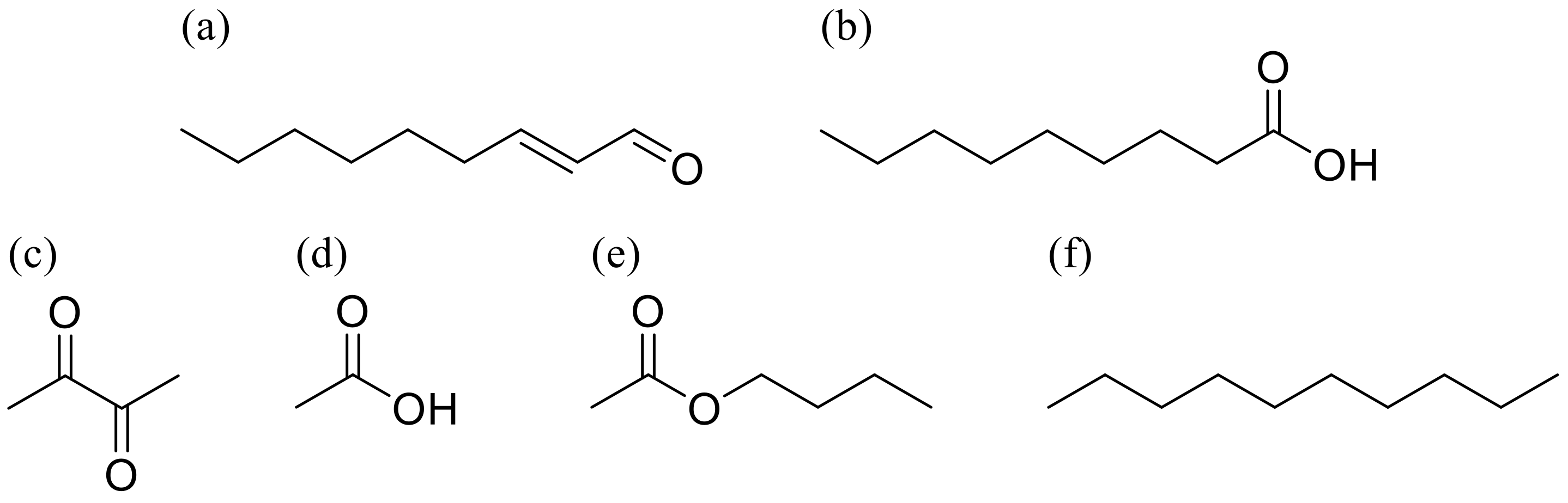
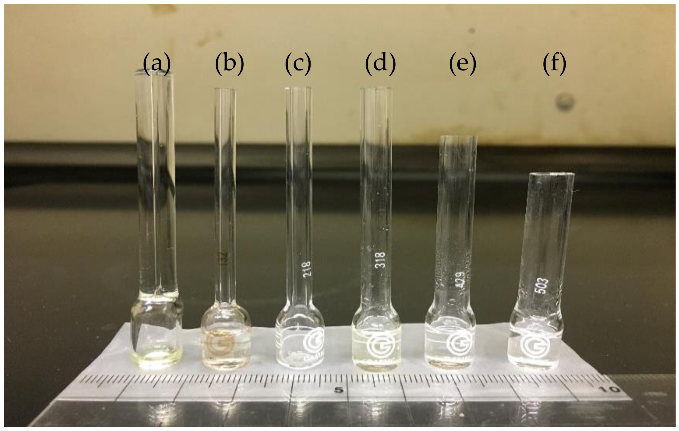
2.2. Preparation of Target and Contaminant VOCs
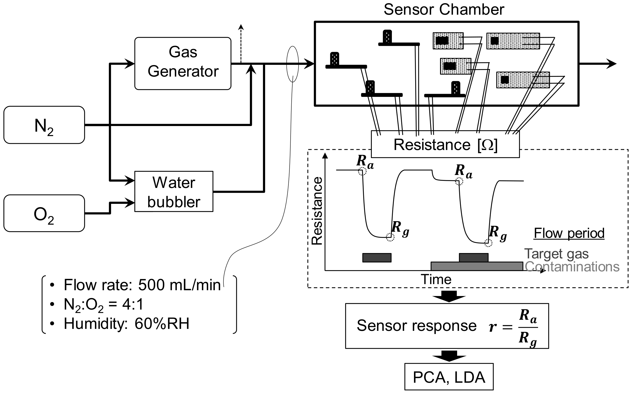
2.3. Gas-Sensor Analysis
2.4. Data Analysis
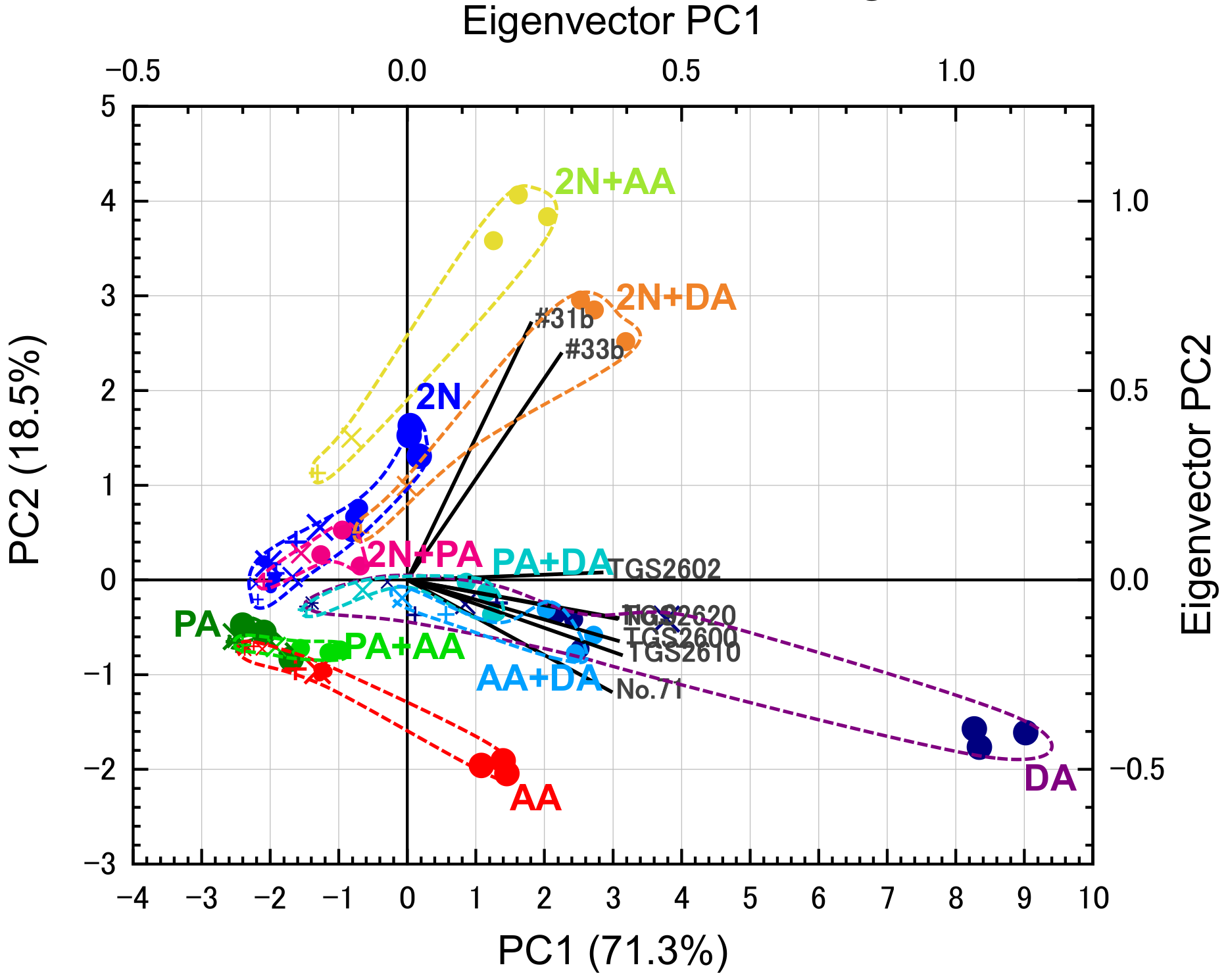
2.4.1. PCA
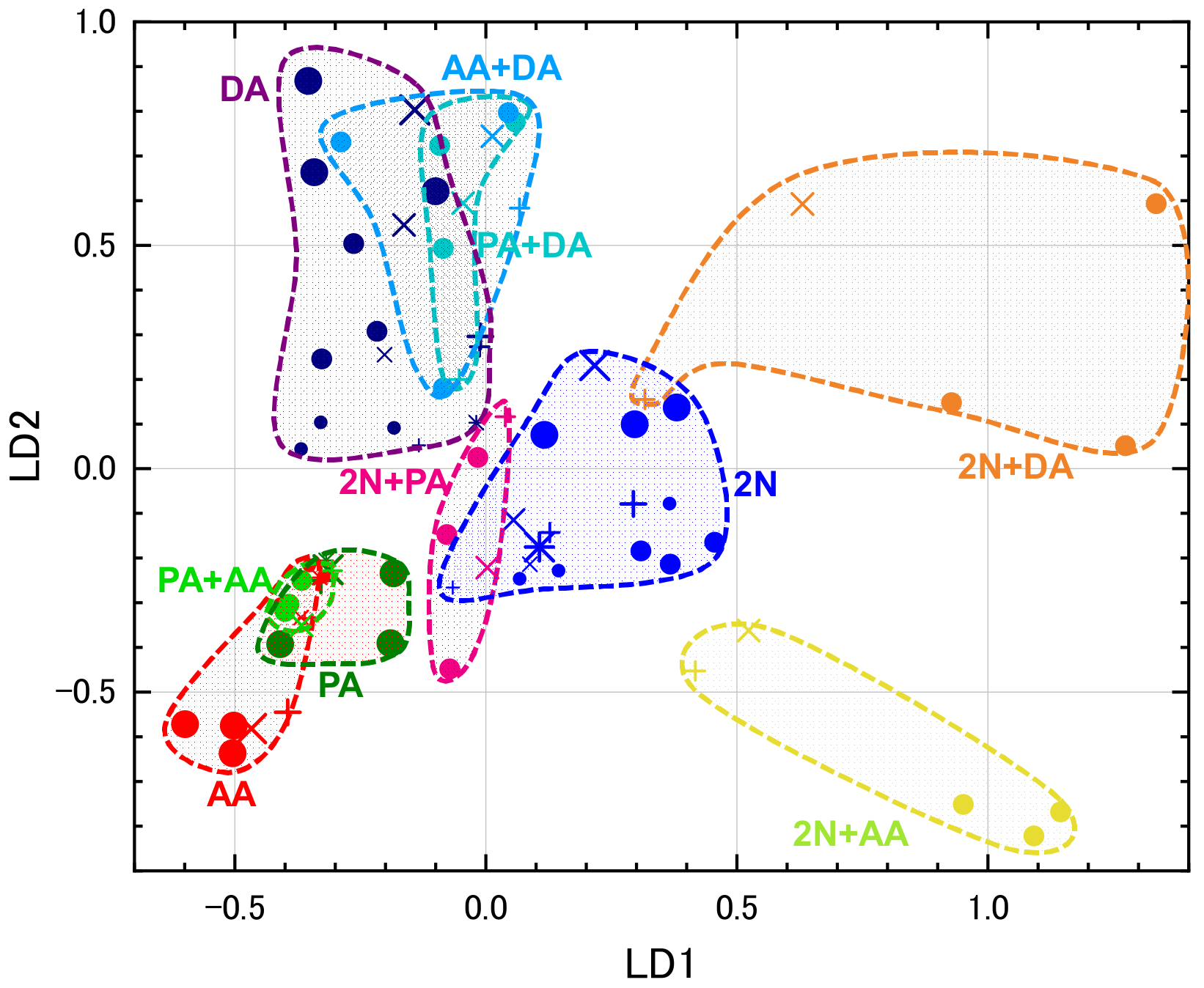
2.4.2. LDA
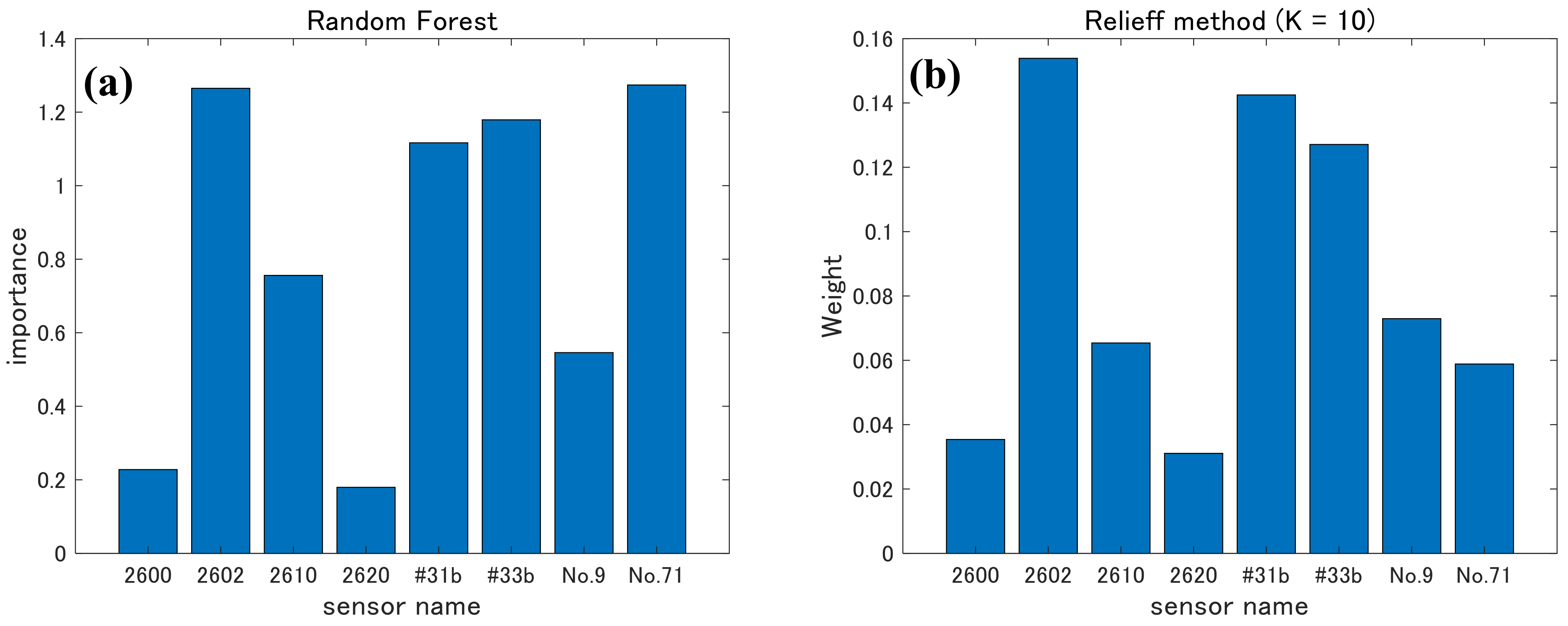
2.4.3. Random Forests and ReliefF
2.4.4. k Nearest Neighbors (kNN)
3. Results and Discussion
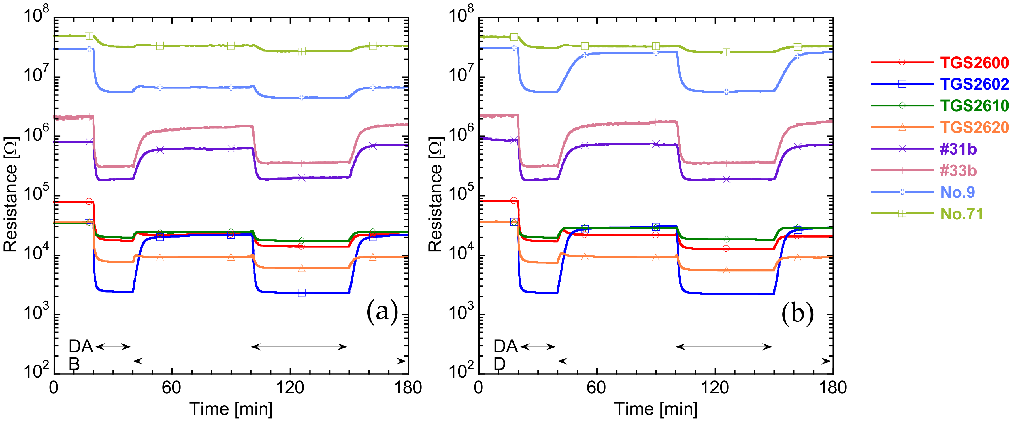
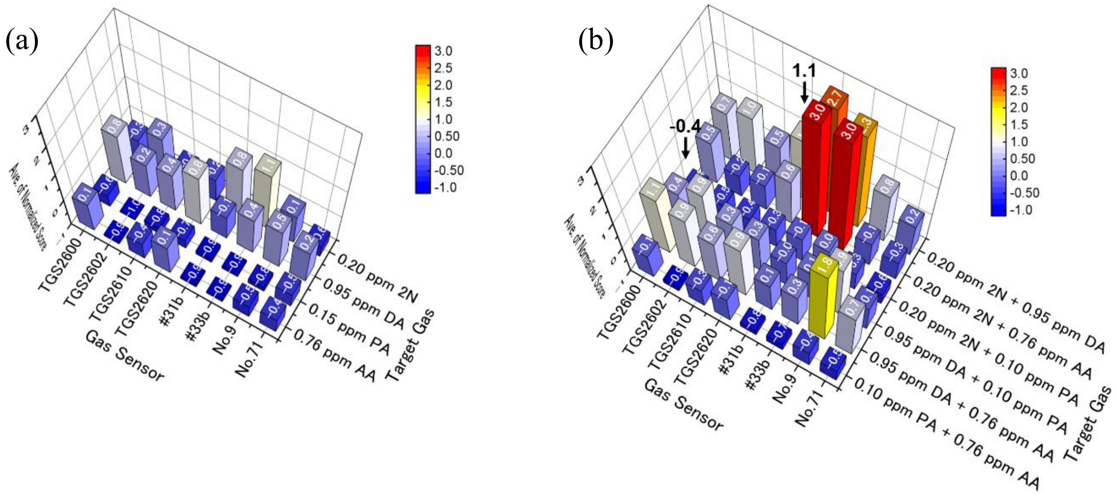
3.1. Sensor Responses and Discrimination of Target Gases
3.2. Selecting Appropriate Sensors for PCA and LDA
4. Conclusions
Author Contributions
Funding
Acknowledgments
Conflicts of Interest
References
- Gozu, Y.; Haze, S.; Nakamura, S.; Kohno, Y.; Fukui, H.; Kumano, Y.; Sawano, K.; Ohta, H.; Yamazaki, K. Development of care-products to prevent aged body odor. J. Soc. Cosmet. Chem. Jpn. 2000, 34, 379–386. (In Japanese) [Google Scholar] [CrossRef]
- Haze, S.; Gozu, Y.; Nakamura, S.; Kohno, Y.; Sawano, K.; Ohta, H.; Yamazaki, K. 2-Nonenal newly found in human body odor tends to increase with aging. J. Investig. Dermatol. 2001, 116, 520–524. [Google Scholar] [CrossRef]
- Ishino, K.; Wakita, C.; Shibata, T.; Toyokuni, S.; Machida, S.; Matsuda, S.; Matsuda, T.; Uchida, K. Lipid peroxidation generates body odor component trans-2-nonenal covalently bound to protein in vivo. J. Biolog. Chem. 2010, 285, 15302–15313. [Google Scholar] [CrossRef]
- Kimura, K.; Sekine, Y.; Furukawa, S.; Takahashi, M.; Oikawa, D. Measurement of 2-nonenal and diacetyl emanating from human skin surface employing passive flux sampler—GCMS system. J. Chromatogr. B 2016, 1028, 181–185. [Google Scholar] [CrossRef]
- Kanda, F.; Yagi, E.; Fukuda, M.; Nakajima, K.; Ohta, T.; Nakata, O.; Fujiyama, Y. Elucidating body malodour to develop a novel body odour quencher. J. Soc. Cosmet. Chem. Jpn. 1989, 23, 217–224. [Google Scholar] [CrossRef]
- Shimizu, H. Development of the deodorization technology corresponding to aging of body odor. Aroma Res. 2014, 15, 146–147. (In Japanese) [Google Scholar]
- Tuomi, T.; Ilvesoksa, J.; Laakso, S.; Rosenqvist, H. Interaction of Abscisic-acid and Indole-3-acetic Acid-Producing Fungi with Salix Levels. J. Plant Growth Regul. 1993, 12, 149–156. [Google Scholar] [CrossRef]
- Simmons, R.B.; Noble, J.A.; Rose, L.; Price, D.L.; Crow, S.A.; Ahearn, D.G. Fungal colonization of automobile air conditioning systems. J. Ind. Microbiol. Biotechnol. 1997, 19, 150–153. [Google Scholar] [CrossRef]
- Simmons, R.B.; Rose, L.J.; Crow, S.A.; Ahearn, D.G. The occurrence and persistence of mixed biofilms in automobile air conditioning systems. Curr. Microbiol. 1999, 39, 141–145. [Google Scholar] [CrossRef]
- Yamazoe, N.; Shimanoe, K. Theory of power laws for semiconductor gas sensors. Sens. Actuators B Chem. 2008, 128, 566–573. [Google Scholar] [CrossRef]
- Yamazoe, N.; Shimanoe, K. New perspectives of gas sensor technology. Sens. Actuators B Chem. 2009, 138, 100–107. [Google Scholar] [CrossRef]
- Izu, N.; Shin, W.; Matsubara, I.; Murayama, N. Development of Resistive Oxygen Sensors Based on Cerium Oxide Thick Film. J. Electroceramics 2004, 13, 703–706. [Google Scholar] [CrossRef]
- Izu, N.; Shin, W.; Matsubara, I.; Murayama, N. Evaluation of response characteristics of resistive oxygen sensors based on porous cerium oxide thick film using pressure modulation method. Sens. Actuators B Chem. 2006, 113, 207–213. [Google Scholar] [CrossRef]
- Itoh, T.; Izu, N.; Akamatsu, T.; Shin, W.; Miki, Y.; Hirose, Y. Elimination of Flammable Gas Effects in Cerium Oxide Semiconductor-Type Resistive Oxygen Sensors for Monitoring Low Oxygen Concentrations. Sensors 2015, 15, 9427–9437. [Google Scholar] [CrossRef]
- Kadosaki, M.; Sakai, Y.; Tamura, I.; Matsubara, I.; Itoh, T. Development of Oxide Semiconductor Thick Film Gas Sensor for the Detection of Total Volatile Organic Compounds. Electro. Commun. Jpn. 2008, 128, 125–130. [Google Scholar] [CrossRef]
- Sakai, Y.; Kadosaki, M.; Matsubara, I.; Itoh, T. Preparation of total VOC sensor with sensor-response stability for humidity by noble metal addition to SnO2. J. Ceram. Soc. Jpn. 2009, 117, 1297–1301. [Google Scholar] [CrossRef]
- Akamatsu, T.I.T.; Tsuruta, A.; Shin, W.; Itoh, T.; Akamatsu, T. Selective Detection of Target Volatile Organic Compounds in Contaminated Humid Air Using a Sensor Array with Principal Component Analysis. Sensors 2017, 17, 1662. [Google Scholar] [CrossRef]
- Byun, H.-G.; Persaud, K.C.; Pisanelli, A.M. Wound-State Monitoring for Burn Patients Using E-Nose/SPME System. ETRI J. 2010, 32, 440–446. [Google Scholar] [CrossRef]
- Yu, J.-B.; Byun, H.-G.; Zhang, S.; Do, S.-H.; Lim, J.O.; Huh, J.-S. Exhaled Breath Analysis of Lung Cancer Patients Using a Metal Oxide Sensor. J. Sens. Sci. Technol. 2011, 20, 300–304. [Google Scholar] [CrossRef]
- Zaromb, S.; Stellar, J.R. Theoretical basis for identification and measurement of air contaminants using an array of sensors having partially overlapping sensitivities. Sens. Actuators 1984, 6, 225–243. [Google Scholar] [CrossRef]
- Imamura, G.; Shiba, K.; Yoshikawa, G. Smell identification of spices using nanomechanical membrane-type surface stress sensors. Jpn. J. Appl. Phys. 2016, 55, 1102B3. [Google Scholar] [CrossRef]
- Güntner, A.T.; Pineau, N.J.; Mochalski, P.; Wiesenhofer, H.; Agapiou, A.; Mayhew, C.A.; Pratsinis, S.E. Sniffing Entrapped Humans with Sensor Arrays. Anal. Chem. 2018, 90, 4940–4945. [Google Scholar] [CrossRef] [PubMed]
- Imamura, G.; Shiba, K.; Yoshikawa, G.; Washio, T. Analysis of nanomechanical sensing signals; physical parameter estimation for gas identification. AIP Adv. 2018, 8, 075007. [Google Scholar] [CrossRef]
- Jeon, J.-Y.; Choi, J.-S.; Yu, J.-B.; Lee, H.-R.; Jang, B.K.; Byun, H.-G. Sensor array optimization techniques for exhaled breath analysis to discriminate diabetics using an electronic nose. ETRI J. 2018, 40, 802–812. [Google Scholar] [CrossRef]
- Kou, L.; Zhang, L.; Liu, D. A Novel Medical E-Nose Signal Analysis System. Sensors 2017, 17, 402. [Google Scholar] [CrossRef]
- Lau, H.-C.; Yu, J.-B.; Lee, H.-W.; Huh, J.-S.; Lim, J.O. Investigation of Exhaled Breath Samples from Patients with Alzheimer’s Disease Using Gas Chromatography-Mass Spectrometry and an Exhaled Breath Sensor System. Sensors 2017, 17, 1783. [Google Scholar] [CrossRef]
- Li, W.; Liu, H.; Xie, D.; He, Z.; Pi, X. Lung Cancer Screening Based on Type-different Sensor Arrays. Sci. Rep. 2017, 7, 1969. [Google Scholar] [CrossRef]
- Cole, M.; Covington, J.A.; Gardner, J. Combined electronic nose and tongue for a flavour sensing system. Sens. Actuators B Chem. 2011, 156, 832–839. [Google Scholar] [CrossRef]
- Itoh, T.; Akamatsu, T.; Izu, N.; Shin, W.; Byun, H.-G. Monitoring of disease-related volatile organic compounds in simulated room air. In Proceedings of the IEEE SENSORS 2014 Proceedings, Valencia, Spain, 2–5 November 2014; pp. 1427–1430. [Google Scholar]
- Itoh, T.; Nakashima, T.; Akamatsu, T.; Izu, N.; Shin, W. Nonanal gas sensing properties of platinum, palladium, and gold-loaded tin oxide VOCs sensors. Sens. Actuators B Chem. 2013, 187, 135–141. [Google Scholar] [CrossRef]
- Bishiop, C.M. Pattern Recognition and Machine Learning; Springer: New York, NY, USA, 2006; Japanese Edition; Maruzen Publishing: Tokyo, Japan, 2012. [Google Scholar]
- Breiman, L. Random Forests. Mach. Learn. 2001, 45, 5–32. [Google Scholar] [CrossRef]
- Millard, K.; Richardson, M. On the Importance of Training Data Sample Selection in Random Forest Image Classification: A Case Study in Peatland Ecosystem Mapping. Remote. Sens. 2015, 7, 8489–8515. [Google Scholar] [CrossRef]
- Menze, B.; Kelm, B.M.; Masuch, R.; Himmelreich, U.; Bachert, P.; Petrich, W.; Hamprecht, F.A. A comparison of random forest and its Gini importance with standard chemometric methods for the feature selection and classification of spectral data. BMC Bioinform. 2009, 10, 213. [Google Scholar] [CrossRef] [PubMed]
- Zhou, Y.; Zhang, R.; Wang, S.; Wang, F. Feature Selection Method Based on High-Resolution Remote Sensing Images and the Effect of Sensitive Features on Classification Accuracy. Sensors 2018, 18, 2013. [Google Scholar] [CrossRef] [PubMed]
- Zhang, J.; Chen, M.; Zhao, S.; Hu, S.; Shi, Z.; Cao, Y. ReliefF-Based EEG Sensor Selection Methods for Emotion Recognition. Sensors 2016, 16, 1558. [Google Scholar] [CrossRef]
- Huang, Y.; Mccullagh, P.; Black, N.D. An optimization of ReliefF for classification in large datasets. Data Knowl. Eng. 2009, 68, 1348–1356. [Google Scholar] [CrossRef]
- Srivastava, A.; Dravid, V.P. On the performance evaluation of hybrid and mono-class sensor arrays in selective detection of VOCs: A comparative study. Sens. Actuators B Chem. 2006, 117, 244–252. [Google Scholar] [CrossRef]


| Sensor Name | Detected Compounds and Sensor Details |
|---|---|
| TGS 2600 | H2 and alcohol (manufactured by Figaro) |
| TGS 2602 | Alcohol, ammonia, VOC, and H2S (manufactured by Figaro) |
| TGS 2610 | Liquefied petroleum gas (manufactured by Figaro) |
| TGS 2620 | Alcohol and solvent vapors (manufactured by Figaro) |
| #31b | VOCs (Pt, Pd, Au/SnO2; film thickness: 4.6 μm) |
| #33b | VOCs (Pt, Pd, Au/SnO2; film thickness: 2.8 μm) |
| No. 9 | Oxygen and VOCs (CeZr10; film thickness: 9 μm) |
| No. 71 | Oxygen and VOCs (CeZr10/Al2O3/Pt-CeZr10; film thickness: 9/4/9 μm) |
| VOCs | Concentration | Selection of D-tubes for Designated Concentration | |
|---|---|---|---|
| Target gas | 2N | 0.20 ppm | D-04 × 1 |
| 0.081 ppm | D-03 × 1 | ||
| 0.021 ppm | D-01 × 1 | ||
| PA | 0.15 ppm | D-05 × 3 | |
| 0.10 ppm | D-05 × 2 | ||
| DA | 5.4 ppm | D-01 × 1 | |
| 1.6 ppm | D-001 × 1 | ||
| 0.95 ppm | D-001* × 1 | ||
| AA | 2.2 ppm | D-01 × 1 | |
| 0.76 ppm | D-001 × 1 | ||
| Contaminant gas | B | 2.7 ppm | D-02 × 1 |
| D | 1.0 ppm | D-04 × 1 |
| Target Gas (Class) | Concentration | Plot Color, Shape, and Size | |||||||
|---|---|---|---|---|---|---|---|---|---|
| Including Contaminant Gases | |||||||||
| None | B (2.7 ppm) | D (1.0 ppm) | B (2.7 ppm) +D (1.0 ppm) | ||||||
| 2N | 0.20 ppm | ● | (large) | + | (large) | × | (large) | * | (large) |
| 0.081 ppm | ● | (medium) | + | (medium) | × | (medium) | * | (medium) | |
| 0.021 ppm | ● | (small) | + | (small) | × | (small) | * | (small) | |
| PA | 0.15 ppm | ● | (large) | + | (large) | × | (large) | * | (large) |
| 0.10 ppm | ● | (small) | + | (small) | × | (small) | * | (small) | |
| DA | 5.4 ppm | ● | (large) | + | (large) | × | (large) | * | (large) |
| 1.6 ppm | ● | (medium) | + | (medium) | × | (medium) | * | (medium) | |
| 0.95 ppm | ● | (small) | + | (small) | × | (small) | * | (small) | |
| AA | 2.2 ppm | ● | (large) | + | (large) | × | (large) | * | (large) |
| 0.76 ppm | ● | (small) | + | (small) | × | (small) | * | (small) | |
| 2N + PA | 0.20 ppm (2N) 0.10 ppm (PA) | ● | (medium) | + | (medium) | × | (medium) | − | − |
| 2N + DA | 0.20 ppm (2N) 0.95 ppm (DA) | ● | (medium) | + | (medium) | × | (medium) | − | − |
| 2N + AA | 0.20 ppm (2N) 0.76 ppm (AA) | ● | (medium) | + | (medium) | × | (medium) | − | − |
| PA + DA | 0.10 ppm (PA) 0.95 ppm (DA) | ● | (medium) | + | (medium) | × | (medium) | − | − |
| PA + AA | 0.10 ppm (PA) 0.76 ppm (AA) | ● | (medium) | + | (medium) | × | (medium) | − | − |
| DA + AA | 0.95 ppm (DA) 0.76 ppm (AA) | ● | (medium) | + | (medium) | × | (medium) | − | − |
| Match Ratio (%) | |||
| Contaminations | |||
| Not included | Included | All | |
| PCA from 8 sensors (Figure 5) | 79 | 74 | 77 |
| LDA from 8 sensors (Figure 7) | 84 | 72 | 79 |
| Match Ratio (%) | |||
| Contamination | |||
| Not included | Included | All | |
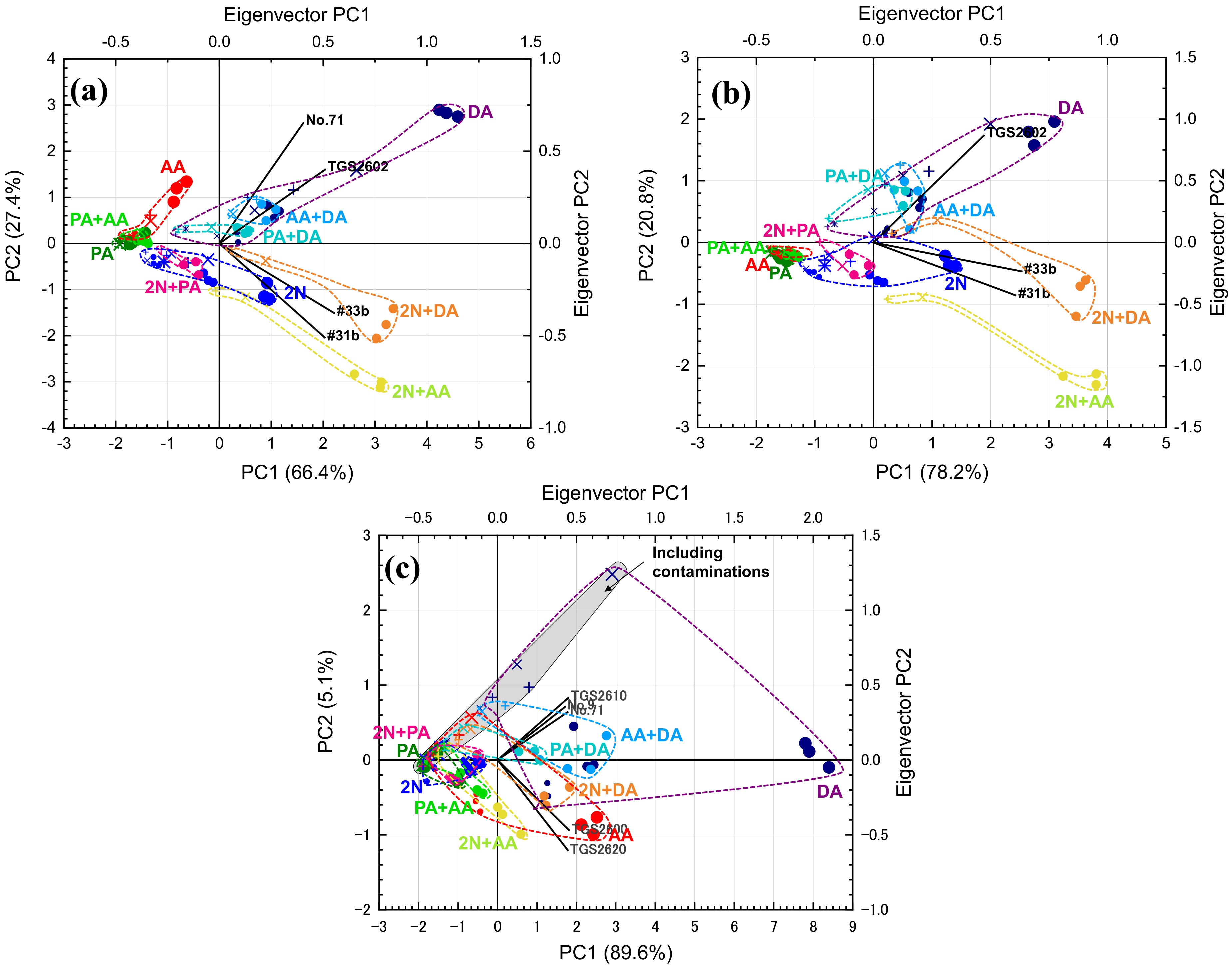
| PCA from 4 sensors (Figure 9a) | 86 | 76 | 82 |
| PCA from 3 sensors (Figure 9b) | 78 | 72 | 75 |
| PCA from 5 sensors (Figure 9c) | 73 | 30 | 55 |
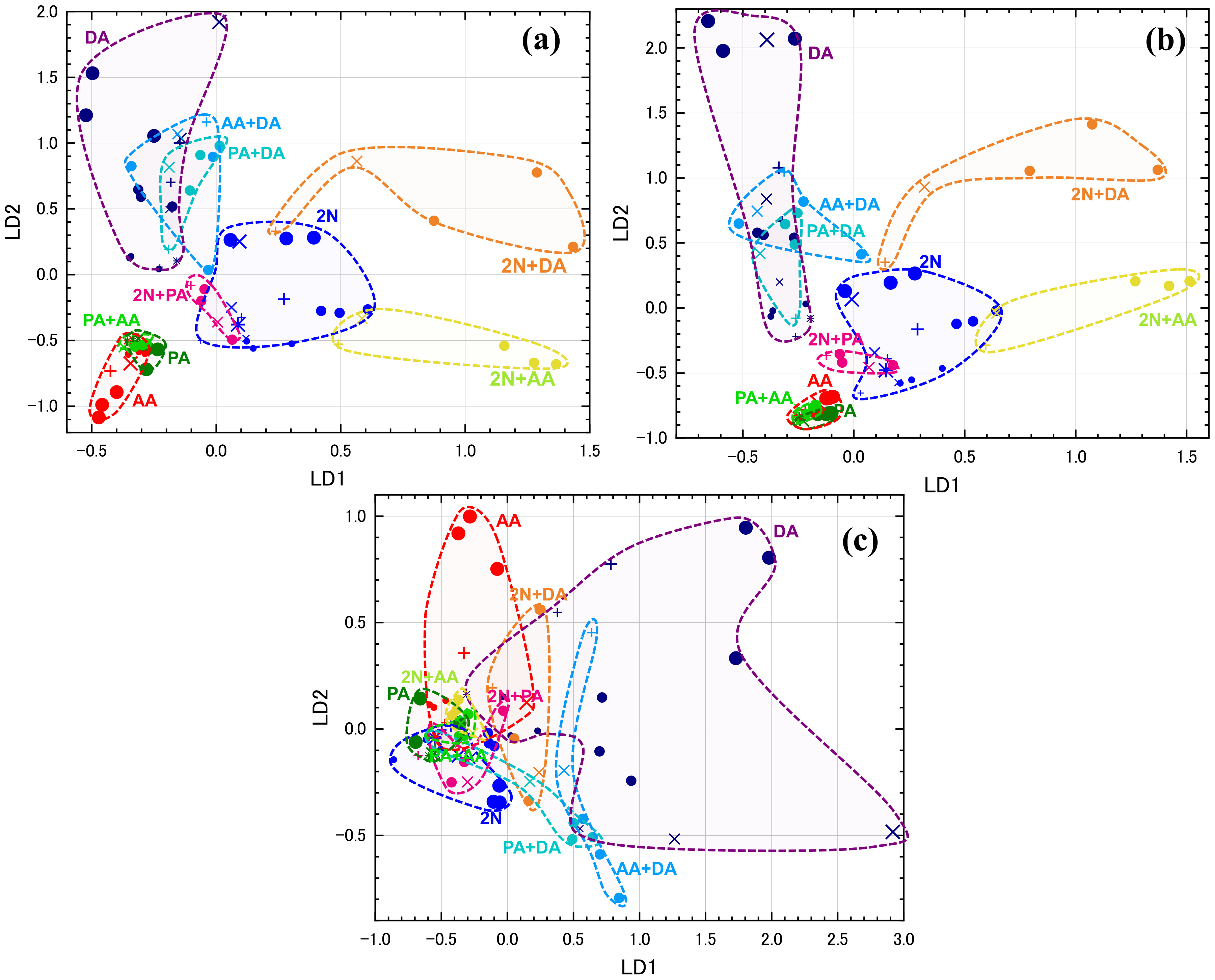
| LDA from 4 sensors (Figure 10a) | 81 | 74 | 78 |
| LDA from 3 sensors (Figure 10b) | 81 | 72 | 77 |
| LDA from 5 sensors (Figure 10c) | 68 | 54 | 62 |
© 2020 by the authors. Licensee MDPI, Basel, Switzerland. This article is an open access article distributed under the terms and conditions of the Creative Commons Attribution (CC BY) license (http://creativecommons.org/licenses/by/4.0/).
Share and Cite
Itoh, T.; Koyama, Y.; Shin, W.; Akamatsu, T.; Tsuruta, A.; Masuda, Y.; Uchiyama, K. Selective Detection of Target Volatile Organic Compounds in Contaminated Air Using Sensor Array with Machine Learning: Aging Notes and Mold Smells in Simulated Automobile Interior Contaminant Gases. Sensors 2020, 20, 2687. https://doi.org/10.3390/s20092687
Itoh T, Koyama Y, Shin W, Akamatsu T, Tsuruta A, Masuda Y, Uchiyama K. Selective Detection of Target Volatile Organic Compounds in Contaminated Air Using Sensor Array with Machine Learning: Aging Notes and Mold Smells in Simulated Automobile Interior Contaminant Gases. Sensors. 2020; 20(9):2687. https://doi.org/10.3390/s20092687
Chicago/Turabian StyleItoh, Toshio, Yutaro Koyama, Woosuck Shin, Takafumi Akamatsu, Akihiro Tsuruta, Yoshitake Masuda, and Kazuhisa Uchiyama. 2020. "Selective Detection of Target Volatile Organic Compounds in Contaminated Air Using Sensor Array with Machine Learning: Aging Notes and Mold Smells in Simulated Automobile Interior Contaminant Gases" Sensors 20, no. 9: 2687. https://doi.org/10.3390/s20092687
APA StyleItoh, T., Koyama, Y., Shin, W., Akamatsu, T., Tsuruta, A., Masuda, Y., & Uchiyama, K. (2020). Selective Detection of Target Volatile Organic Compounds in Contaminated Air Using Sensor Array with Machine Learning: Aging Notes and Mold Smells in Simulated Automobile Interior Contaminant Gases. Sensors, 20(9), 2687. https://doi.org/10.3390/s20092687