Classification for Penicillium expansum Spoilage and Defect in Apples by Electronic Nose Combined with Chemometrics

 ,
, 


 and
and
Abstract
1. Introduction
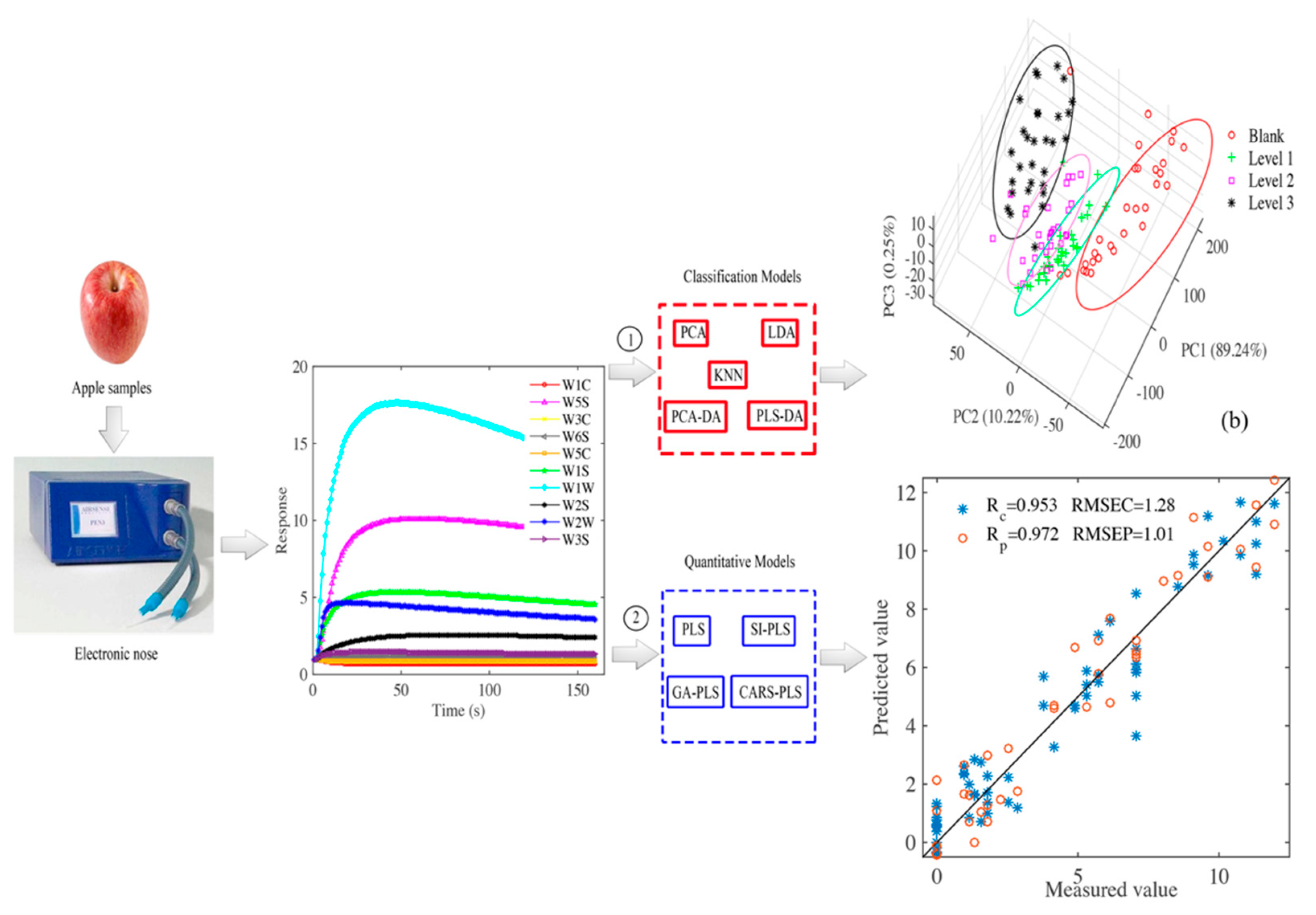
2. Materials and Methods
2.1. Sample Preparation
2.2. Electronic Nose Sampling
2.3. Pattern Recognition Methods
2.3.1. Principal Component Analysis
2.3.2. Linear Discriminant Analysis
2.3.3. K-Nearest Neighbor
2.3.4. Principal Component Analysis Discriminant Analysis
2.3.5. Partial Least Square Discriminant Analysis
2.4. Multivariate Calibration Methods
2.4.1. Partial Least Square
2.4.2. Synergy Interval Partial Least Square
2.4.3. Genetic Algorithm
2.4.4. Competitive Adaptive Reweighted Sampling
3. Results and Analysis
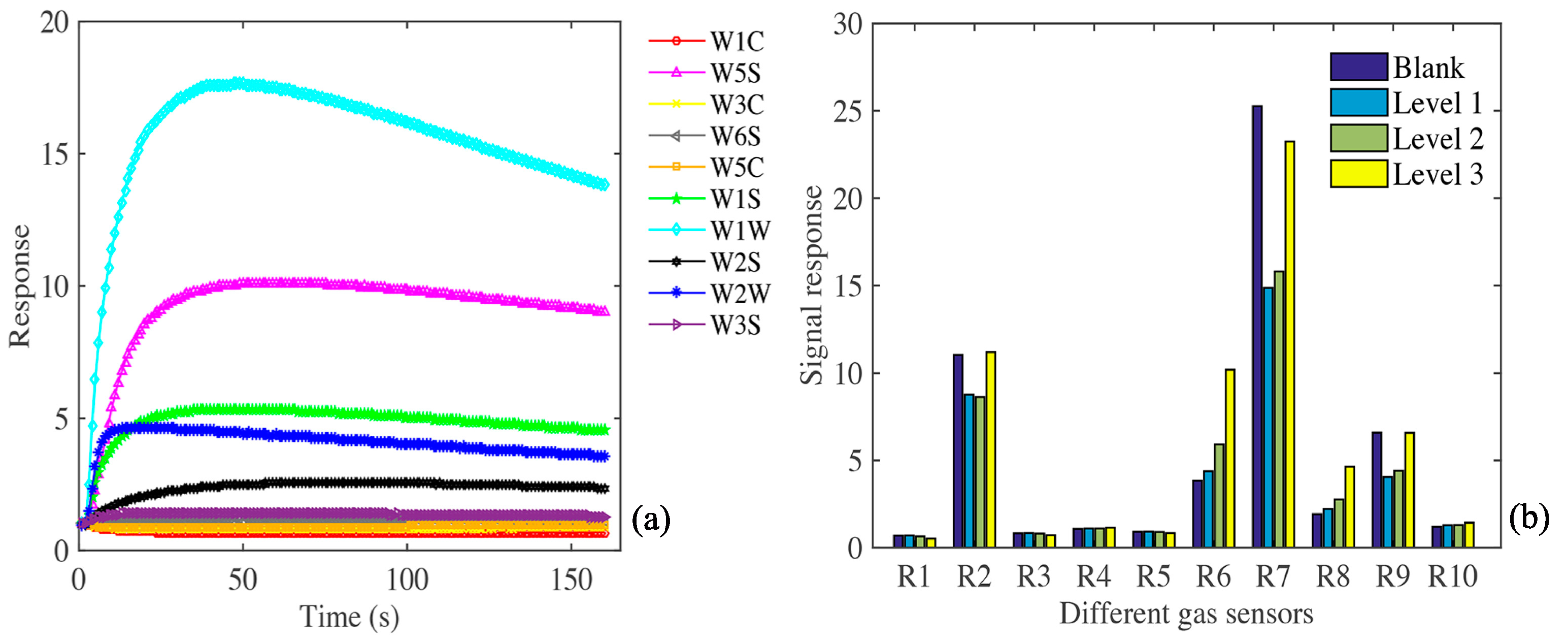
3.1. Analysis of Apple Gas Components
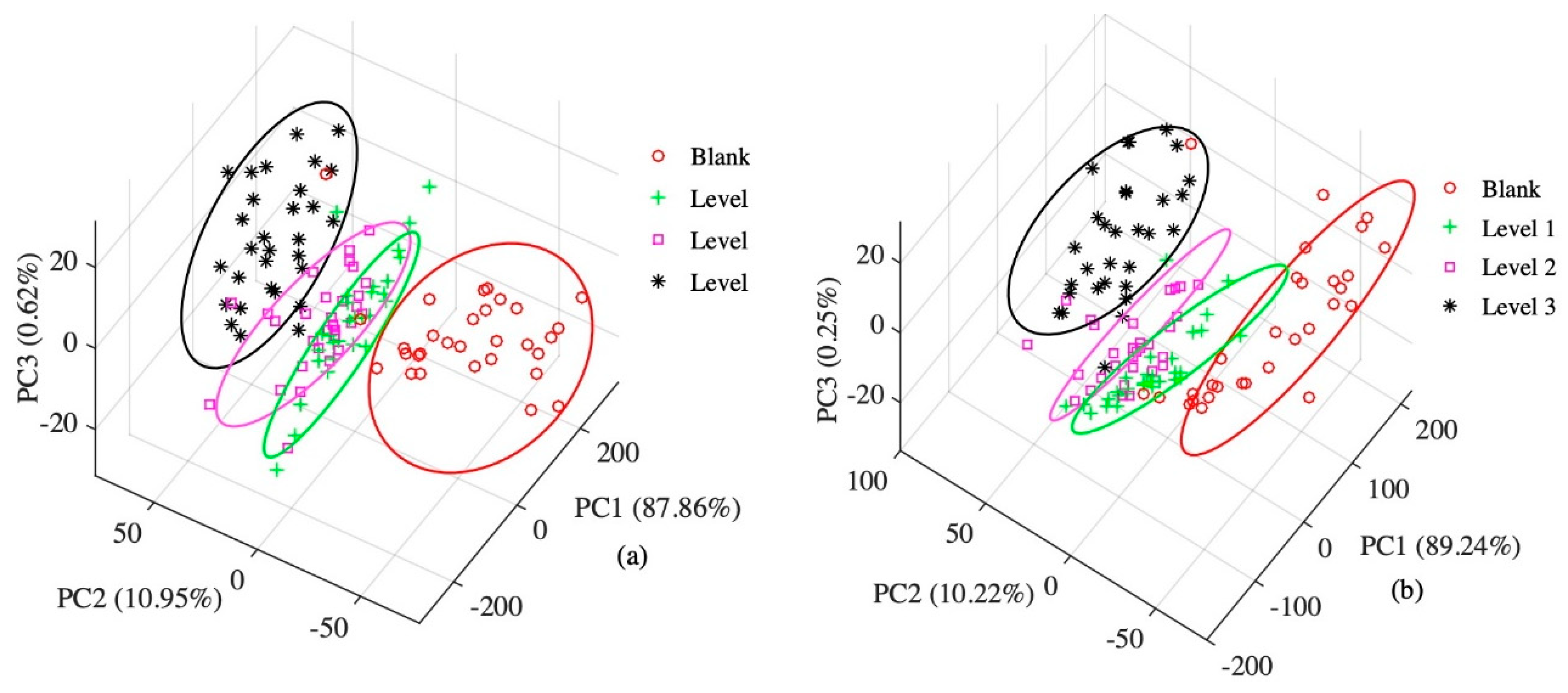
3.2. Principal Component Analysis
3.3. Classification Models of Spoilage
3.3.1. LDA Model
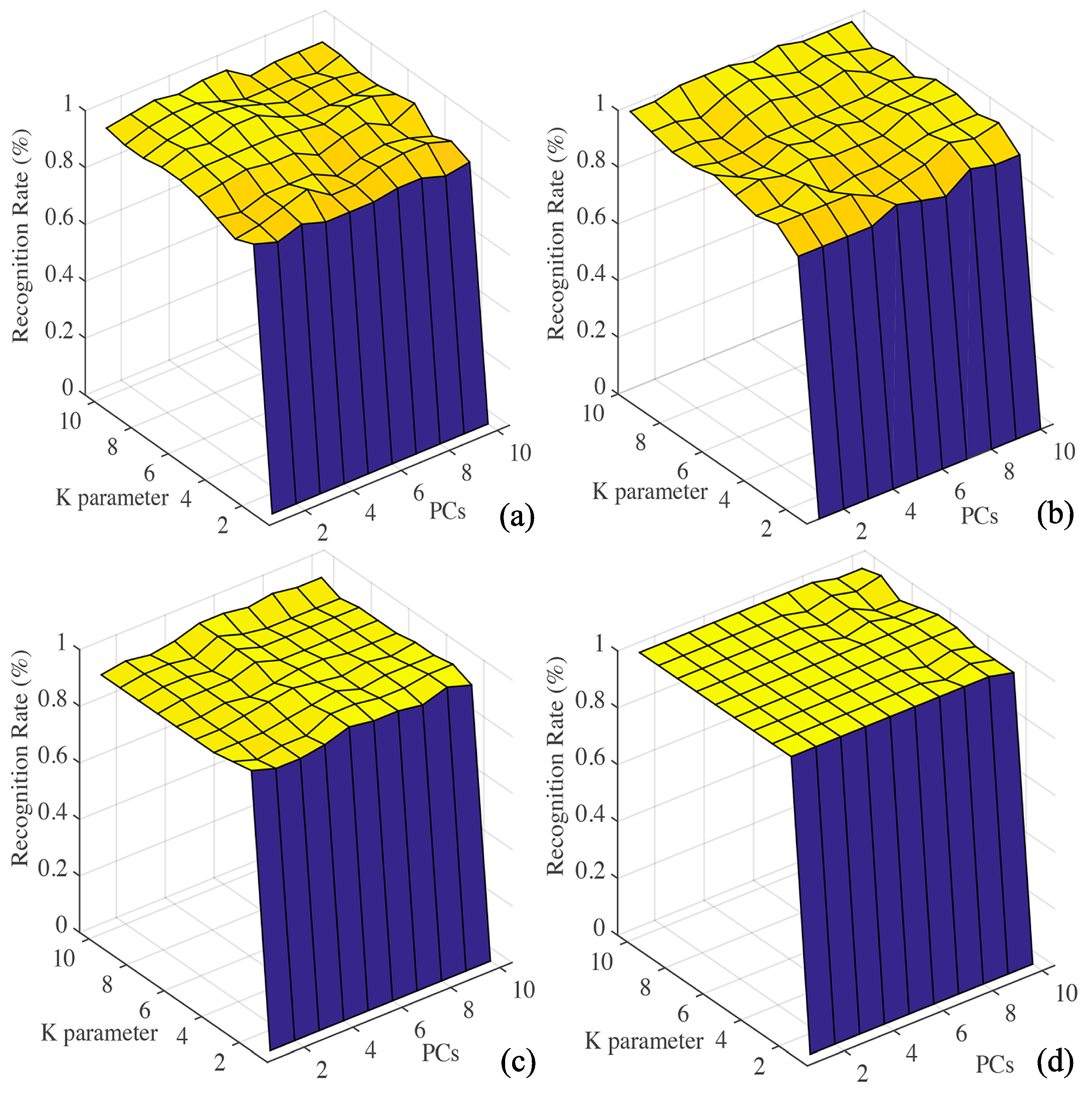
3.3.2. KNN Model
3.3.3. PCA-DA Model
3.3.4. PLS-DA Model
3.3.5. Compare Different Classification Algorithms
3.4. Quantitative Models of Apple Spoilage Area
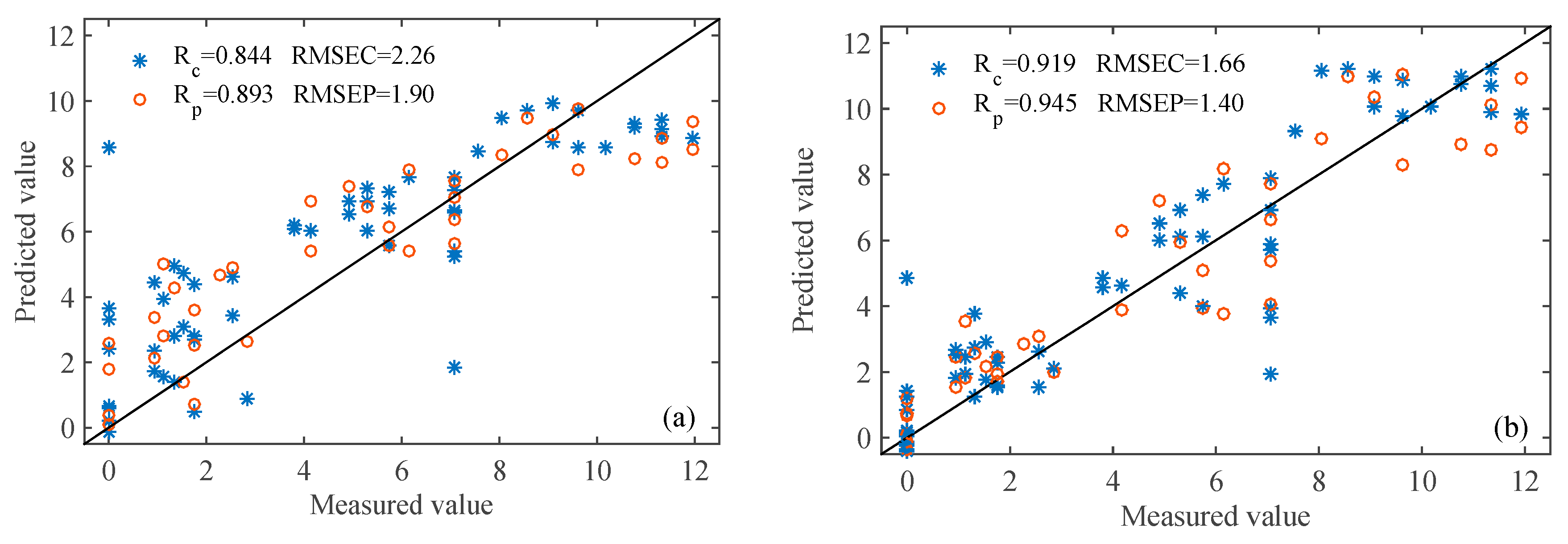
3.4.1. PLS Models
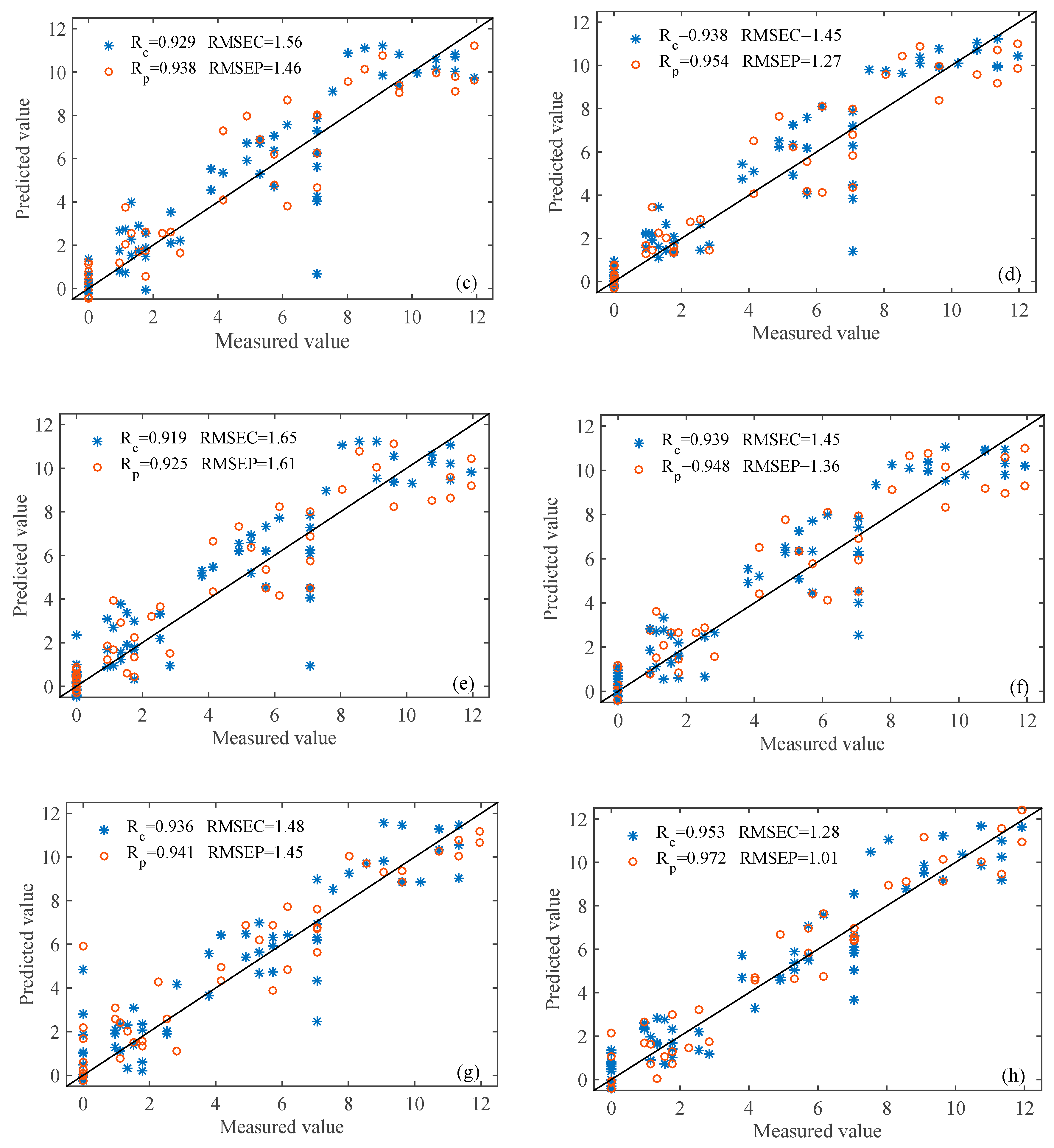
3.4.2. SI-PLS Models
3.4.3. GA-PLS Models
3.4.4. CARS-PLS Models
3.4.5. Comparisons of Different PLS Models.
4. Conclusions
Supplementary Materials
Author Contributions
Funding
Conflicts of Interest
References
- FAO food and agriculture statistic. 2018. Available online: http://www.fao.org/faostat/en/#data/QC (accessed on 1 February 2020).
- Mastello, R.B.; Capobiango, M.; Chin, S.-T.; Monteiro, M.; Marriott, P.J. Identification of odour-active compounds of pasteurised orange juice using multidimensional gas chromatography techniques. Food Res. Int. 2015, 75, 281–288. [Google Scholar] [CrossRef] [PubMed]
- Pelletier, A.; Lavoie, J.-M.; Chornet, E. Identification of secondary metabolites in citrus fruit using gas chromatography and mass spectroscopy. J. Chem. Educ. 2008, 85, 1555. [Google Scholar] [CrossRef]
- Bhargava, A.; Bansal, A. Quality evaluation of Mono & bi-Colored Apples with computer vision and multispectral imaging. Multimed Tools Appl. 2020, 1–18. [Google Scholar]
- Guo, Z.; Huang, W.; Peng, Y.; Chen, Q.; Ouyang, Q.; Zhao, J. Color compensation and comparison of shortwave near infrared and long wave near infrared spectroscopy for determination of soluble solids content of ‘Fuji’ apple. Postharvest Biol. Tec. 2016, 115, 81–90. [Google Scholar] [CrossRef]
- Berna, A. Metal Oxide Sensors for Electronic Noses and Their Application to Food Analysis. Sensors 2010, 10, 3882–3910. [Google Scholar] [CrossRef]
- Shi, H.; Zhang, M.; Adhikari, B. Advances of electronic nose and its application in fresh foods: A review. Crit. Rev. Food Sci. 2018, 58, 2700–2710. [Google Scholar] [CrossRef]
- Dai, C.; Huang, X.; Huang, D.; Lv, R.; Sun, J.; Zhang, Z.; Ma, M.; Aheto, J.H. Detection of submerged fermentation of Tremella aurantialba using data fusion of electronic nose and tongue. J. Food Process Eng. 2019, 42, e13002. [Google Scholar] [CrossRef]
- Ying, X.; Liu, W.; Hui, G. Litchi freshness rapid non-destructive evaluating method using electronic nose and non-linear dynamics stochastic resonance model. Bioengineered 2015, 6, 218–221. [Google Scholar] [CrossRef]
- Xu, S.; Lu, E.; Lu, H.; Zhou, Z.; Wang, Y.; Yang, J.; Wang, Y. Quality Detection of Litchi Stored in Different Environments Using an Electronic Nose. Sensors 2016, 16, 852. [Google Scholar] [CrossRef]
- Dai, C.; Huang, X.; Lv, R.; Zhang, Z.; Sun, J.; Aheto, J.H. Analysis of volatile compounds of Tremella aurantialba fermentation via electronic nose and HS-SPME-GC-MS. J. Food Saf. 2018, 38, e12555. [Google Scholar] [CrossRef]
- Torri, L.; Sinelli, N.; Limbo, S. Shelf life evaluation of fresh-cut pineapple by using an electronic nose. Postharvest Biol. Technol. 2010, 56, 239–245. [Google Scholar] [CrossRef]
- Sun, J.; Zhang, R.; Zhang, Y.; Liang, Q.; Li, G.; Yang, N.; Xu, P.; Guo, J. Classifying fish freshness according to the relationship between EIS parameters and spoilage stages. J. Food Eng. 2018, 219, 101–110. [Google Scholar] [CrossRef]
- Adak, M.F.; Yumusak, N. Classification of E-nose aroma data of four fruit types by ABC-based neural network. Sensors 2016, 16, 304. [Google Scholar] [CrossRef] [PubMed]
- Güney, S.; Atasoy, A. Study of fish species discrimination via electronic nose. Comput. Electron Agr. 2015, 119, 83–91. [Google Scholar] [CrossRef]
- Pan, L.; Zhang, W.; Zhu, N.; Mao, S.; Tu, K. Early detection and classification of pathogenic fungal disease in post-harvest strawberry fruit by electronic nose and gas chromatography–mass spectrometry. Food Res. Int. 2014, 62, 162–168. [Google Scholar] [CrossRef]
- Bonah, E.; Huang, X.; Yi, R.; Aheto, J.H.; Osae, R.; Golly, M. Electronic nose classification and differentiation of bacterial foodborne pathogens based on support vector machine optimized with particle swarm optimization algorithm. J. Food Process Eng. 2019, 42, e13236. [Google Scholar] [CrossRef]
- Bonah, E.; Huang, X.; Aheto, J.H.; Osae, R. Application of electronic nose as a non-invasive technique for odor fingerprinting and detection of bacterial foodborne pathogens: a review. J. Food Sci. Technol. 2019, 1–14. [Google Scholar] [CrossRef]
- Biondi, E.; Blasioli, S.; Galeone, A.; Spinelli, F.; Cellini, A.; Lucchese, C.; Braschi, I. Detection of potato brown rot and ring rot by electronic nose: From laboratory to real scale. Talanta 2014, 129, 422–430. [Google Scholar] [CrossRef]
- Bro, R.; Smilde, A.K. Principal component analysis. Anal. Methods 2014, 6, 2812–2831. [Google Scholar] [CrossRef]
- Li, C.-N.; Shao, Y.-H.; Deng, N.-Y. Robust L1-norm two-dimensional linear discriminant analysis. Neural Netw. 2015, 65, 92–104. [Google Scholar] [CrossRef]
- Tharwat, A.; Gaber, T.; Ibrahim, A.; Hassanien, A.E. Linear discriminant analysis: A detailed tutorial. AI Commun. 2017, 30, 169–190. [Google Scholar] [CrossRef]
- Peterson, L.E. K-nearest neighbor. Scholarpedia 2009, 4, 1883. [Google Scholar] [CrossRef]
- Lee, M.; Gatton, T.M.; Lee, K.-K. A monitoring and advisory system for diabetes patient management using a rule-based method and KNN. Sensors 2010, 10, 3934–3953. [Google Scholar] [CrossRef] [PubMed]
- Maione, C.; Barbosa, F., Jr.; Barbosa, R.M. Predicting the botanical and geographical origin of honey with multivariate data analysis and machine learning techniques: A review. Comput. Electron. Agr. 2019, 157, 436–446. [Google Scholar] [CrossRef]
- Górski, Ł.; Kowalcze, M.; Jakubowska, M. Classification of six herbal bioactive compositions employing LAPV and PLS-DA. J. Chemom. 2019, 33, e3112. [Google Scholar] [CrossRef]
- Feng, X.; Zhao, Y.; Zhang, C.; Cheng, P.; He, Y. Discrimination of transgenic maize kernel using NIR hyperspectral imaging and multivariate data analysis. Sensors 2017, 17, 1894. [Google Scholar] [CrossRef]
- Lin, H.M.; Lee, M.H.; Liang, J.C.; Chang, H.Y.; Huang, P.; Tsai, C.C. A review of using partial least square structural equation modeling in e-learning research. Br. J. Educ. Technol. 2019. [Google Scholar] [CrossRef]
- Nørgaard, L.; Saudland, A.; Wagner, J.; Nielsen, J.P.; Munck, L.; Engelsen, S.B. Interval partial least-squares regression (i PLS): A comparative chemometric study with an example from near-infrared spectroscopy. Appl. Spectrosc. 2000, 54, 413–419. [Google Scholar] [CrossRef]
- Guo, Z.; Wang, M.; Agyekum, A.A.; Wu, J.; Chen, Q.; Zuo, M.; El-Seedi, H.R.; Tao, F.; Shi, J.; Ouyang, Q. Quantitative detection of apple watercore and soluble solids content by near infrared transmittance spectroscopy. J. Food Eng. 2020, 109955. [Google Scholar] [CrossRef]
- Leardi, R. Application of genetic algorithm–PLS for feature selection in spectral data sets. J. Chemom. 2000, 14, 643–655. [Google Scholar] [CrossRef]
- Men, H.; Shi, Y.; Fu, S.; Jiao, Y.; Qiao, Y.; Liu, J. Mining feature of data fusion in the classification of beer flavor information using e-tongue and e-nose. Sensors 2017, 17, 1656. [Google Scholar]
- Da Silva, D.J.; Wiebeck, H. CARS-PLS regression and ATR-FTIR spectroscopy for eco-friendly and fast composition analyses of LDPE/HDPE blends. J. Polym. Res. 2018, 25, 112. [Google Scholar] [CrossRef]


| Number in Array | Sensor | Main Attribute | Typical Target |
|---|---|---|---|
| R1 | W1C | Aromatic compounds | C6H5CH3 |
| R2 | W5S | Nitrogen oxides | NO2 |
| R3 | W3C | Ammonia and aromatic molecules | C6H6 |
| R4 | W6S | Hydrogen | H2 |
| R5 | W5C | Alkanes, aromatic compounds | C3H8 |
| R6 | W1S | Broad methane | CH4 |
| R7 | W1W | Sulfur-containing organics | H2S |
| R8 | W2S | Broad alcohols | C2H5OH |
| R9 | W2W | Aromatics, organic sulfides | H2S |
| R10 | W3S | Methane and aliphatics | CH4 |
| Algorithm | All Sensors (R1-R10) | Feature Sensors (R2 R6 R7 R9) | ||
|---|---|---|---|---|
| Calibration Set | Prediction Set | Calibration Set | Prediction Set | |
| LDA | 98.61% | 95.83% 5.83% | 95.83% | 95.83% |
| KNN | 98.61% | 95.83% | 95.83% | 100% |
| PCA-DA | 95.83% | 95.83% | 97.22% | 100% |
| PLS-DA | 100% | 93.75% | 95.83% | 100% |
| Model | All Sensors (R1-R10) | Feature Sensors (R2 R6 R7 R9) | ||||||
|---|---|---|---|---|---|---|---|---|
| Calibration Set | Prediction Set | Calibration Set | Prediction Set | |||||
| Rc | RMSEC | RP | RMSEP | Rc | RMSEC | RP | RMSEP | |
| PLS | 0.844 | 2.26 | 0.893 | 1.90 | 0.919 | 1.66 | 0.945 | 1.40 |
| SI-PLS | 0.929 | 1.56 | 0.938 | 1.46 | 0.938 | 1.45 | 0.954 | 1.27 |
| GA-PLS | 0.917 | 1.65 | 0.925 | 1.61 | 0.939 | 1.44 | 0.942 | 1.42 |
| CARS-PLS LSPLS | 0.937 | 1.48 | 0.941 | 1.45 | 0.953 | 1.28 | 0.972 | 1.01 |
© 2020 by the authors. Licensee MDPI, Basel, Switzerland. This article is an open access article distributed under the terms and conditions of the Creative Commons Attribution (CC BY) license (http://creativecommons.org/licenses/by/4.0/).
Share and Cite
Guo, Z.; Guo, C.; Chen, Q.; Ouyang, Q.; Shi, J.; El-Seedi, H.R.; Zou, X. Classification for Penicillium expansum Spoilage and Defect in Apples by Electronic Nose Combined with Chemometrics. Sensors 2020, 20, 2130. https://doi.org/10.3390/s20072130
Guo Z, Guo C, Chen Q, Ouyang Q, Shi J, El-Seedi HR, Zou X. Classification for Penicillium expansum Spoilage and Defect in Apples by Electronic Nose Combined with Chemometrics. Sensors. 2020; 20(7):2130. https://doi.org/10.3390/s20072130
Chicago/Turabian StyleGuo, Zhiming, Chuang Guo, Quansheng Chen, Qin Ouyang, Jiyong Shi, Hesham R. El-Seedi, and Xiaobo Zou. 2020. "Classification for Penicillium expansum Spoilage and Defect in Apples by Electronic Nose Combined with Chemometrics" Sensors 20, no. 7: 2130. https://doi.org/10.3390/s20072130
APA StyleGuo, Z., Guo, C., Chen, Q., Ouyang, Q., Shi, J., El-Seedi, H. R., & Zou, X. (2020). Classification for Penicillium expansum Spoilage and Defect in Apples by Electronic Nose Combined with Chemometrics. Sensors, 20(7), 2130. https://doi.org/10.3390/s20072130