Monitoring Winter Stress Vulnerability of High-Latitude Understory Vegetation Using Intraspecific Trait Variability and Remote Sensing Approaches

Abstract

In this study, we focused on three species that have proven to be vulnerable to winter stress: Empetrum nigrum, Vaccinium vitis-idaea and Hylocomium splendens. Our objective was to determine plant traits suitable for monitoring plant stress as well as trait shifts during spring. To this end, we used a combination of active and passive handheld normalized difference vegetation index (NDVI) sensors, RGB indices derived from ordinary cameras, an optical chlorophyll and flavonol sensor (Dualex), and common plant traits that are sensitive to winter stress, i.e. height, specific leaf area (SLA). Our results indicate that NDVI is a good predictor for plant stress, as it correlates well with height (r = 0.70, p < 0.001) and chlorophyll content (r = 0.63, p < 0.001). NDVI is also related to soil depth (r = 0.45, p < 0.001) as well as to plant stress levels based on observations in the field (r = −0.60, p < 0.001). Flavonol content and SLA remained relatively stable during spring. Our results confirm a multi-method approach using NDVI data from the Sentinel-2 satellite and active near-remote sensing devices to determine the contribution of understory vegetation to the total ecosystem greenness. We identified low soil depth to be the major stressor for understory vegetation in the studied plots. The RGB indices were good proxies to detect plant stress (e.g. Channel G%: r = −0.77, p < 0.001) and showed high correlation with NDVI (r = 0.75, p < 0.001). Ordinary cameras and modified cameras with the infrared filter removed were found to perform equally well.

1. Introduction

Global warming will affect arctic and subarctic regions more than any other area in the world [1]. It is expected to increase the productivity of subarctic and arctic ecosystems [2,3,4]. Increasing productivity and biomass is generally known as ‘greening’ [5]. Major drivers are a longer growing season and increasing summer warming [6]. However, negative trends in productivity and biomass, known as ‘browning’, have also been reported [6]. For the Arctic as a whole, trends are complex, as Myers-Smith et al. state: “Figures vary from 42% greening and 2.5% browning from 1982 to 2014 in the GIMMS3g AVHRR dataset to 20% greening and 4% browning from 2000 to 2016 in Landsat data, and to estimates of 13% greening and 1% browning for the MODIS trends calculated for 1,000 random points in the tundra polygon from 2000 to 2018.” ([7], p. 107).

In the subarctic region of Scandinavia, i.e. Norway, Finland, and Sweden north of the Arctic Circle, the main drivers of browning are winter warming events and pest outbreaks [8]. Winter warming events can melt the insulating snow cover that normally protects photosynthetic short-statured organisms overwintering with aboveground tissue (e.g. prostrate shrubs, cushion plants, bryophytes, and lichens) from the harsh ambient winter weather conditions. After a few thaw days, ground vegetation becomes exposed to ambient air and hibernation is interrupted, thus reducing the protection of photosynthetic organisms against frost, which may easily lead to freezing damage upon return of normal winter weather [9]. Soil communities, including both micro-arthropods and bacteria, can also be severely affected [10]. Overall, a warmer winter climate changes species compositions and reduces carbon cycling [11]. In subarctic and arctic regions evergreen plants in particular are sensitive to changing winter climate and reduced snow cover [12]. This includes the widespread dwarf shrubs Empetrum nigrum L., Vaccinium vitis-idaea L., Cassiope tetragona (L.) D.Don, and Calluna vulgaris (L.) Hull, as well as the tall coniferous shrub Juniperus communis L. [6,11,13]. Bryophytes, such as the widespread feathermoss Hylocomium splendens (Hedw.) Schimp., deciduous shrubs, such as Vaccinium myrtillus L., evergreen horsetails (Equisetum spp.), as well as small cushion plants show reduced growth following exposure to winter warming [9,11,13,14]. The other major factor causing browning are pest outbreaks. Recently, increasing frequency and intensity of outbreaks of leaf-defoliating geometrid moths led to massive canopy defoliation of their preferred host tree Betula pubescens Ehrh. and understory plants [13,15,16]. Overall, multiple stress events are main drivers of browning. Given the high focus on climate change-induced changes in northern primary productivity, it is important to develop easy and reliable methods for assessment of plant vitality.

For a long time, satellites have monitored the global vegetation status [2,3,17]. Spectral sensors operated near the target vegetation are increasingly applied for assessing the plant status [18,19]. However, near-remote time series of the plant status are still uncommon, which is partly due to the need for expensive equipment, for example spectroradiometers [20]. In recent years, several new and low-cost active and passive proximal sensors were developed. This includes sensors measuring the normalized difference vegetation index (NDVI). NDVI is a radiometric measure of the amount of radiation (≈∼400–700 nm) absorbed by vegetation during photosynthesis. It is calculated from contrasting reflectance at near-infrared (NIR) and red bands [21,22].

NDVI has been widely used in studies of phenology, productivity, biomass, and disturbance monitoring, as it has proven to be a good proxy of the vegetation’s photosynthetic activity [19,23]. NDVI works well for subarctic ecosystem monitoring and is widely used on different scales and as a vegetation marker [24,25,26].

Previously, modified cameras—with the infrared filter removed—were found to be good NDVI surrogates. In such cameras, the NDVI proxy is commonly calculated by using the enhanced red channel and the blue channel (BNDVI) [27]. However, a combination of the enhanced red channel and the green channel might also be of interest due to a strong linear correlation with the chlorophyll content (GNDVI) [28]. Additionally, ordinary cameras were increasingly applied for vegetation analysis and phenology studies in recent years. Greenness indices based on ordinary RGB images from such cameras are promising NDVI substitutes [28,29], even for high-arctic vegetation [30].

In subarctic forests, the contribution of understory vegetation (i.e. dwarf shrubs, herbs, graminoids, bryophytes and lichens) to the total ecosystem productivity is similar to that of trees [31]. Moreover, biodiversity of vascular plants at high latitudes is relatively low, which makes research into dominant species and their vulnerability to environmental change even more important [32]. We hypothesized that in situ estimates of plant damage would be correlated to optical measurements of plant greenness, but that greenness indices would vary in their explanatory power. Our second hypothesis was that plant stress would vary over short distances in a rolling subarctic landscape and that this would be detectable both by near-remote sensing measurements and by Sentinel. To this end, we combined near-remote sensing approaches with classical determination of plant traits of understory vegetation to address the following research questions:

(1)

What is the range of intraspecific variability of common traits of dwarf shrubs and mosses in subarctic spring?

(2)

Which traits are reliable indicators of plant stress?

(3)

How do the indices derived from ordinary and modified RGB cameras correlate with common plant traits?

To answer these questions, we made analyses in a widespread subarctic heath ecosystem, focusing on vegetation plots dominated by two evergreen dwarf shrubs and a mat-forming moss.

2. Materials and Methods

2.1. Site Description

We selected plots in wind-exposed areas where snow cover generally is shallow and plants are more susceptible to winter frost-thaw stress. Eighteen plots (1 m × 1 m) were assessed within a total area of approx. 1 km² in Tromsø, Troms County, northern Norway (Figure S1, Table S1, Figure S2b,c). Satellite upscaling was conducted in homogeneous plots within a wider area in Tromsø (Table S2), from 8–12 June 2017, corresponding to days of year (DOY) 159–163. The three areas (a total of ca. 0.5 ha) for the upscaling approach were not congruent to the eighteen field plots (a total of 18 m²). We chose three separate areas in order to avoid trails, snow patches, unvegetated ground and rocky steep slopes (as exemplified in Figure S2a). Unvegetated ground was estimated to be around 10% in the area shown in Figure S2a. The other two areas had around 5% of unvegetated ground. Satellite upscaling was performed when snow patches became sparse, but before budburst of the deciduous trees in the heath. The study focuses on the evergreen dwarf shrub species Empetrum nigrum and Vaccinium vitis-idaea and the mat-forming moss Hylocomium splendens. These species are abundant, co-occur in boreal ecosystems, and are linked to browning [9,14,33]. Our continuous monitoring of plant vitality in the study area shows that these species have not been exposed to severely stressful events since 2012, as reported in Bjerke et al. [15]. Minor damage rates were recorded in more recent years, then mostly restricted to wind-exposed sites with little snow accumulation (unpublished observations). Thus, plant traits in the study area were expected to vary naturally along microclimatic gradients. Plots with different stress levels (or health states) were established for each species to monitor natural intraspecific trait variabilities. The studied plots were dominated by (with number of plots in parentheses): V. vitis-idaea (two), H. splendens (three), E. nigrum (nine), and mixed plots of E. nigrum with a lower layer of H. splendens (four).

2.2. Data Collection

Five greenness measurements were made in each plot (n = 87) from DOY 130 to DOY 180. Weather conditions varied between days of measurements. For greenness measurements we used four handheld spectral devices (Table 1). The Mapir NDVI camera was only accessible in the last two sampling cycles (n = 35). All passive spectral devices were applied 1.5 to 2.0 m above the plot for photographing. We avoided photographing direct light reflectance in the calibration target, and also avoided overexposure. The active Greenseeker sensor measurements were acquired 60 cm above ground.

Measurements of epidermal chlorophyll and flavonol content were conducted with the optical Dualex 4 scientific instrument (Force-A, Orsay, France). The readings of this instrument show a linear relationship to chlorophyll concentrations calculated from extractions. Readings are given in μg cm⁻², and the measuring wavelength for chlorophyll is a ratio of transmittance at 710 and 850 nm [34]. Within each plot, we sampled at five different spots. The sampling dates were the same as for the greenness measurements. Measurements were made on the newest, fully developed segment of H. splendens and on shoot tips of E. nigrum. Eight V. vitis-idaea leaves of one plant were measured per sample, starting with the upper (= newer) leaves. Hence, we measured physiological traits in different health states on three plots per species (nine in total). All measurements were performed with the adaxial setting of the device. High correlations with the abaxial side are found [35]. Measurements of V. vitis-idaea leaves showed reliable results. However, for the shoots of H. splendens, stable and reproducible results could only be achieved when three shoots were stacked and fixed with a transparent tape (Figure S3b). The same process was used for the shoots of E. nigrum (Figure S3a). At least eight chlorophyll measurements were performed on each sample and readings were then averaged and divided by the number of stacks in the tape. This results in 40 measurements per sampling date and plot. Palta [36] identified leaf anatomy, leaf veins, the presence of other pigments, and leaf thickness as main causes of large variations in chlorophyll meter readings. Hence, we decided to take the specific leaf area (SLA) into account. SLA is also of additional value to determine growth and plant stress [37,38]. After the chlorophyll measurements had been performed, a 6 mm circle was punched out of the prepared samples (Figure S3) [39]. First, fresh weight of the samples was measured. Then, the samples were dried for 24 h at 70 °C before dry weight was measured. This provided information on moisture content and SLA. Plant height was measured as median height above ground. Plant height of H. splendens refers to the thickness of the moss layer. We assessed stress levels for each plot in the first and last sampling periods. The stress estimate is a bare-eye classification of visibly dead or dying leaves versus healthy leaves of evergreens within small plots. Leaves that are dead or dying are brown, while healthy leaves are green. The stress estimate thus ranges from 0 to 100%, and it has turned out to be closely correlated to NDVI [13] and CO₂ fluxes [40].

2.3. Data Processing

2.3.1. Greenness Indices

We applied four different devices and extracted six different greenness indices from these (Table 1). The calibration methods applied are also listed. The Greenseeker did not need a calibration; internal tests suggest that measurements are not dependent on environmental changes [41].

Table 1. Background information on the greenness indices used in this study. Market prices refer to price levels in 2019.

Name	Equation	Device	Market Price	Calibration	Comments	Source
Greenseeker NDVI	Automatically calculated NDVI output; range 0–1 1	GreenSeeker handheld crop sensor (Trimble Inc., Sunnyvale, CA, USA)	ca. 700 $	Not needed	Active sensor	[41,42]
Mapir NDVI	$\frac{\mathrm{NIR}-\mathrm{Red}}{\mathrm{NIR}+\mathrm{Red}}$	Survey2 Camera – NDVI (Mapir Inc., San Diego, CA, USA)	ca. 400 $	Mapir target	Passive sensor	[43]
BNDVI	$\frac{\mathrm{Red}-\mathrm{Blue}}{\mathrm{Red}+\mathrm{Blue}}$	Modified Canon Eos 450D (no IR filter) (MaxMax, LDP LLC, Carlstadt, CA, USA)	Body + conversion = 250 $	White balance (WB) on gray area 2	Widely used NDVI surrogate	[44]
GNDVI	$\frac{\mathrm{Red}-\mathrm{Green}}{\mathrm{Red}+\mathrm{Green}}$	Same as for BNDVI	Same as for BNDVI	White balance (WB) on gray area 2	More linear correlation with chlorophyll than NDVI	[28,29]
GRVI	$\frac{\mathrm{Green}-\mathrm{Red}}{\mathrm{Green}+\mathrm{Red}}$	α7 (ILCE-7) (Sony Corp., Tokyo, Japan)	ca. 700 $, but could be any RGB camera	3-step gray card 2, when EV = −0.7	RGB index	[45]
Channel G%	$\frac{\mathrm{Green}}{\mathrm{Red}+\mathrm{Green}+\mathrm{Blue}}$	Same as for GRVI	Same as for GRVI	3-step gray card and white balance on white area 2 when EV = −0.7	RGB index	[46,47]

¹ According to the manufacturer’s documents, even non-chlorophyll-containing surfaces, such as soil, have small NDVI values. Therefore, values below 0.15 are rarely measured. Likewise, normal NDVI, with a range from −1 to 1, shows NDVI values between 0.00 and 0.12 for scarce vegetation or bare soil. ² Ordinary gray card with (N2, N5, N9.5) with an accuracy of about 5% on the Macbeth color space.

Table 1. Background information on the greenness indices used in this study. Market prices refer to price levels in 2019.

Name	Equation	Device	Market Price	Calibration	Comments	Source
Greenseeker NDVI	Automatically calculated NDVI output; range 0–1 1	GreenSeeker handheld crop sensor (Trimble Inc., Sunnyvale, CA, USA)	ca. 700 $	Not needed	Active sensor	[41,42]
Mapir NDVI	$\frac{\mathrm{NIR}-\mathrm{Red}}{\mathrm{NIR}+\mathrm{Red}}$	Survey2 Camera – NDVI (Mapir Inc., San Diego, CA, USA)	ca. 400 $	Mapir target	Passive sensor	[43]
BNDVI	$\frac{\mathrm{Red}-\mathrm{Blue}}{\mathrm{Red}+\mathrm{Blue}}$	Modified Canon Eos 450D (no IR filter) (MaxMax, LDP LLC, Carlstadt, CA, USA)	Body + conversion = 250 $	White balance (WB) on gray area 2	Widely used NDVI surrogate	[44]
GNDVI	$\frac{\mathrm{Red}-\mathrm{Green}}{\mathrm{Red}+\mathrm{Green}}$	Same as for BNDVI	Same as for BNDVI	White balance (WB) on gray area 2	More linear correlation with chlorophyll than NDVI	[28,29]
GRVI	$\frac{\mathrm{Green}-\mathrm{Red}}{\mathrm{Green}+\mathrm{Red}}$	α7 (ILCE-7) (Sony Corp., Tokyo, Japan)	ca. 700 $, but could be any RGB camera	3-step gray card 2, when EV = −0.7	RGB index	[45]
Channel G%	$\frac{\mathrm{Green}}{\mathrm{Red}+\mathrm{Green}+\mathrm{Blue}}$	Same as for GRVI	Same as for GRVI	3-step gray card and white balance on white area 2 when EV = −0.7	RGB index	[46,47]

¹ According to the manufacturer’s documents, even non-chlorophyll-containing surfaces, such as soil, have small NDVI values. Therefore, values below 0.15 are rarely measured. Likewise, normal NDVI, with a range from −1 to 1, shows NDVI values between 0.00 and 0.12 for scarce vegetation or bare soil. ² Ordinary gray card with (N2, N5, N9.5) with an accuracy of about 5% on the Macbeth color space.

The spectral properties of the devices we used for NDVI calculation are listed in

Table 2. Comparison of spectral properties of the various NDVI devices listed in Table 1. Numbers in parentheses show the bandwidth in nanometers.

	Mapir	Greenseeker	Sentinel-2	Sentinel-2	Sentinel-2
	Survey 2 NDVI	Handheld Crop Sensor	Band 4	Band 7	Band 8
Red band	660 nm (50)	660 nm (25)	665 nm (30)
NIR band	850 nm (70)	780 nm (25)		783 nm (20)	833 nm (106)
Spatial resolution	16 MP camera	an oval depending on the height of the sensor: at 60 cm, length is 25 cm	10 m	20 m	10 m

. The active Greenseeker device has very similar bandwidths and -peaks to the Sentinel-2 bands 4 and 7. The spectral properties of the passive Mapir camera are closer to the “normal” NDVI calculated with Sentinel-2 bands 4 and 8.

2.3.2. Analysis of the Data

For the calibration of the RGB indices as well as of BNDVI and GNDVI, an ordinary gray card was applied. The card is printed on Teslin Synthetic (greywhitebalancecolorcard, Northfleet, UK]. According to the manufacturer, it has an accuracy of 5% on the Macbeth color space. To decide whether a three-step reflectance calibration on black, gray, and white is superior to a normal white balance, the Channel G% index was calculated for both calibrations. For the Mapir camera (Mapir Inc., San Diego, CA, USA) conversion and calibration were performed with the Mapir calibration target V1 and the QGIS software plug-in version 1.1.2. (Mapir Inc.). All other calibrations and NDVI calculations were performed in WINCAM pro 2013a (Regent Instruments Inc., Quebec City, QC, Canada). Further processing was done in EXCEL (Microsoft Corp., Redmond, WA, USA), while statistical analyses were performed with SPSS 25.0. (IBM Corp., Armonk, NY, USA). Additional, logistic curve fitting was analyzed using the Excel add-on Xlfit version 5.3.1.3 (ID Business Solutions Ltd., Guildford, UK). We calculated all correlations with a two-tailed Pearson´s testimony. Percentiles are weighted averages. Satellite NDVI data were retrieved from ESA’s Sentinel-2 Open Access Hub [https://scihub.copernicus.eu]. Sentinel-2 satellite images were analyzed using ESA’s SNAP software version 5.0.8 with the integrated Sentinel-2 Toolbox (ESA, Common Service Section, Rome, Italy). Atmospherically corrected 2A products from DOY 159 and DOY 163 in 2017 were used. Cloud cover was below 1% and products were analyzed with a resampled spatial resolution of 20 m. Downscaling was done with the “mean method,” which calculates the output as mean of every source pixel value. The downscaling was performed to compare the different bands of Sentinel-2 for a pixelwise NDVI comparison, and also to reduce small-scale effects, like imprecise GPS coordinates (up to 3 m). To compare spaceborne and handheld NDVI data, at least four GPS waypoints were taken per area and NDVI values between the waypoints were measured with the Greenseeker handheld sensor (Trimble Inc., Sunnyvale, CA, USA, see Table S2). The sensor can also be used for measurement over a larger area. Then, it calculates an average of the scanned area. The Sentinel-2 image pixels corresponding to the GPS waypoints were identified and values were compared with the Greenseeker data.

3. Results

3.1. Descriptive Statistics

Descriptive statistics of the vegetation indices and plant traits are listed in

Table 3. Descriptive statistics of the monitored plant traits on plot level.

Name	Mean	Std. Error	Std. Deviation	N	5% PCTL	Median	95% PCTL	Skewness	Kurtosis
Greenseeker NDVI	0.64	0.0099	0.092	88	0.48	0.63	0.80	0.018	−0.701
Mapir NDVI	0.69	0.0104	0.062	35	0.56	0.69	0.78	−0.611	0.246
BNDVI	0.86	0.0096	0.090	88	0.68	0.87	0.99	−0.569	−0.233
Channel G%	0.40	0.0050	0.047	87	0.48	0.39	0.80	0.848	0.283
GRVI	−0.098	0.0087	0.081	88	−0.212	−0.108	0.072	0.659	0.349
GNDVI	0.47	0.0085	0.079	88	0.34	0.47	0.60	−0.395	0.393
Plant height	9.46	0.0638	4.508	50	4.00	8.25	19.00	0.748	−0.430
Stress level	32.07	4.6593	27.956	36	0.85	30.00	93.63	1.009	0.274
Soil depth	13.73	0.7238	6.790	88	4.00	12.00	25.00	0.267	−1.301
SLA	0.149	0.0151	0.093	38	0.059	0.103	0.343	0.993	−0.238
Chl	23.46	0.7151	4.401	38	15.28	22.92	32.78	−0.014	0.617
Flav	1.01	0.0672	0.414	38	0.61	0.81	1.86	1.065	−0.420
NBI	25.31	0.0151	7.241	38	14.34	25.93	36.04	−0.018	−1.166

. Due to relatively large sampling sizes (n > 36) for all traits on plot level we can assume that data is normally distributed. The combination of three different species in one dataset (Table 3), might lead to less normal distributed data. According a Kolmogorov-Smirnov test, all datasets of Table 1 are normally distributed (p > 0.05), except for Channel G%, Plant height, Stress level, Soil depth, SLA and Flav. However, a species-specific normal distribution is achieved for Plant height, NBI, SLA and Flav. For Channel G% the species-specific normal distribution does not hold for V. vitis-idaea, which was monitored on only two plots with highly contrasting stress levels. Stress level in total is not expected to be normally distributed due to plot selection by contrasting health states. Moreover, Soil depth is also not expected to be normally distributed.

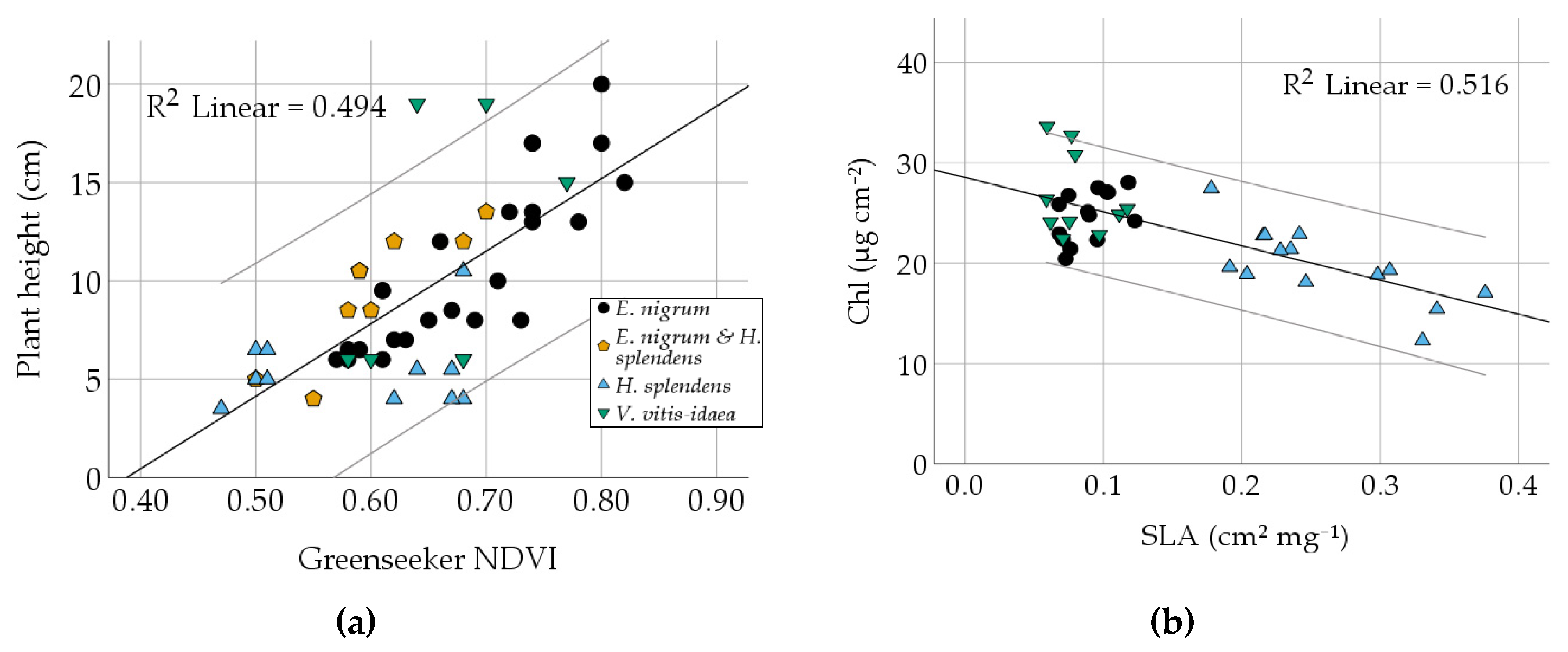
3.2. Comparison of Different Vegetation Indices and Plant Traits

We assessed the use of the six greenness indices and the different calibration methods. Accuracy was not found to be improved by using a relatively cheap 3-step reflectance target instead of an ordinary gray card for white balance (Table S3). However, it was important to avoid overexposure of the calibration target. Comparing the greenness indices (

Table 4. Correlations between greenness indices and plant traits at plot level. Root Mean Squared Error (RMSE) of the linear regressions (slope, intercept) is computed for significant correlations with r > 0.4. Chl = chlorophyll content, Flav = flavonol absorbance, and NBI = nitrogen balance index, i.e. the ratio between Chl and Flav.

		BNDVI	Channel G%	GRVI	GNDVI	Plant Height	Stress Level	Soil Depth	SLA	Chl	Flav	NBI
NDVI	Correlation	0.779	0.749	0.689	0.440	0.703	−0.600	0.454	−0.451	0.634	0.260	0.190
	Sig.	0.000	0.000	0.000	0.000	0.000	0.000	0.000	0.004	0.000	0.116	0.254
	RMSE	0.0571	0.0314	0.0592	0.0716	3.2404	22.682	6.086	0.0841	3.4572
	Slope/ Intercept	0.762/0.376	0.379/0.159	0.606/−0.485	0.377/0.232	36.892/−14.313	−188.3/ 152.9	33.324/ −7.562	−0.446/ 0.436	29.706/ 4.320
	N	88	87	88	88	50	36	88	38	38	38	38
BNDVI	Correlation		0.730	0.641	0.547	0.468	−0.654	0.246	−0.232	0.433	−0.029	0.327
	Sig.		0.000	0.000	0.000	0.001	0.000	0.021	0.161	0.007	0.863	0.045
	RMSE		0.0324	0.0627	0.0668	4.026	21.469			4.027
	slope/intercept		0.378/0.076	0.576/ −0.595	0.480/0.059	26.478/ −13.720	−233.09/228.97			19.167/ 7.033
	N		87	88	88	50	36	88	38	38	38	38
Channel G%	Correlation			0.909	0.454	0.515	−0.768	0.395	−0.141	0.376	−0.051	0.354
	Sig.			0.000	0.000	0.000	0.000	0.000	0.397	0.020	0.759	0.029
	RMSE			0.0340	0.0714	3.946	18.176
	Slope/Intercept			1.565/ −0.728	0.164/0.768	49.185/ −10.268	−419.85/203.61
	N			87	87	49	36	87	38	38	38	38
GRVI	Correlation				0.338	0.554	−0.745	0.393	−0.124	0.387	0.019	0.301
	Sig.				0.001	0.000	0.000	0.000	0.459	0.016	0.908	0.066
	RMSE					3.7909	18.909
	slope/intercept					30.426/12.371	−246.65/11.770
	N				88	50	36	88	38	38	38	38
GNDVI	Correlation					0.045	−0.220	0.070	−0.324	0.226	−0.120	0.294
	Sig.					0.758	0.196	0.515	0.047	0.172	0.472	0.074
	N					50	36	88	38	38	38	38
Plant height	Correlation						−0.553	0.425	−0.357	0.365	0.383	−0.160
	Sig.						0.001	0.002	0.103	0.095	0.079	0.477
	RMSE						22.129	6.3474
	slope/intercept						−3.085/58.926	0.654/ 7.765
	N						34	50	22	22	22	22
Stress level	Correlation							−0.336	−0.110	−0.232	−0.090	−0.021
	Sig.							0.045	0.707	0.425	0.760	0.944
	N							36	14	14	14	14
Soil depth	Correlation								−0.025	0.103	−0.441	0.685
	Sig.								0.883	0.539	0.006	0.000
	RMSE										0.3768	5.3469
	slope/intercept										−0.027/ 1.385	0.721/ 15.182
	N								38	38	38	38
SLA	Correlation									−0.718	−0.512	0.086
	Sig.									0.000	0.001	0.607
	RMSE									3.1102	0.3605
	slope/intercept									−34.048/28.541	−2.282/ 1.353
	N									38	38	38
Chl	Correlation										0.541	0.045
	Sig.										0.000	0.790
	RMSE										0.3530
	slope/intercept										0.051/−0.180
	N										38	38
Flav	Correlation											−0.787
	Sig.											0.000
	RMSE											4.5306
	slope/intercept											−13.759/39.239
	N											38

): Mapir NDVI and Greenseeker NDVI were significantly correlated (r = 0.951, p < 0.001; Figure 1a), while ordinary RGB indices showed a much lower correlation, albeit still significant. NDVI to BNDVI (r = 0.779, p < 0.001) correlated slightly better than Channel G% to NDVI (r = 0.749, p < 0.001) and NDVI to GRVI (r = 0.689, p < 0.001). Greenseeker NDVI showed the best correlation with the chlorophyll content (r = 0.634; p < 0.001), while other indices, such as BNDVI, showed rather low correlations with the chlorophyll content (r = 0.433, p < 0.01; Table 4). Figure 1 illustrates the results for different species and how they correlate with the other indices. Comparison of BNDVI and Greenseeker NDVI (Figure 1b) reveals several high BNDVI values around 1 and increased deviation of lower values. Moreover, spaceborne NDVI data from the Sentinel-2 satellites based on band 4/7/8 (Figure 1e,f) are highly correlated with ground-sampled NDVI values (r = 0.956 and r = 0.968, p < 0.001, n = 14) obtained using the Greenseeker device. In principle, this allows for a significant upscaling from ground to space.

Joint analyses of all plant species resulted in variable correlations between the greenness indices and other plant traits, i.e. SLA, chlorophyll content, and plant height (Table 4). The nitrogen index (NBI) shows a good correlation with soil depth (r = 0.685, p < 0.001), indicating that the nutrients may be limited by shallow soil depths. The NDVI and the Channel G% indices allow for an assumption of plant height, as correlations are good (NDVI: r = 0.703, p < 0.001; Channel G%: r = 0.515, p < 0.001), even when comparing across functional groups, i.e. by considering mosses and dwarf shrubs together. Species-specific correlations are listed in Tables S5–S8. Specifically, the correlation (Figure 2b) between SLA and chlorophyll (r = −0.718, p < 0.001) is almost solely driven by the moss H. splendens, which shows a strong correlation when analyzed separately (r = −0.745, p < 0.01), whereas V. vitis-idaea and E. nigrum showed no significant correlation. A similar case is the SLA to flavonol correlation (r = −0.512, p = 0.001; Table 4). In this case, E. nigrum is the only species showing a significant correlation when analyzed species-wise (r = −0.589, p < 0.05), while the two other species showed no significant correlation.

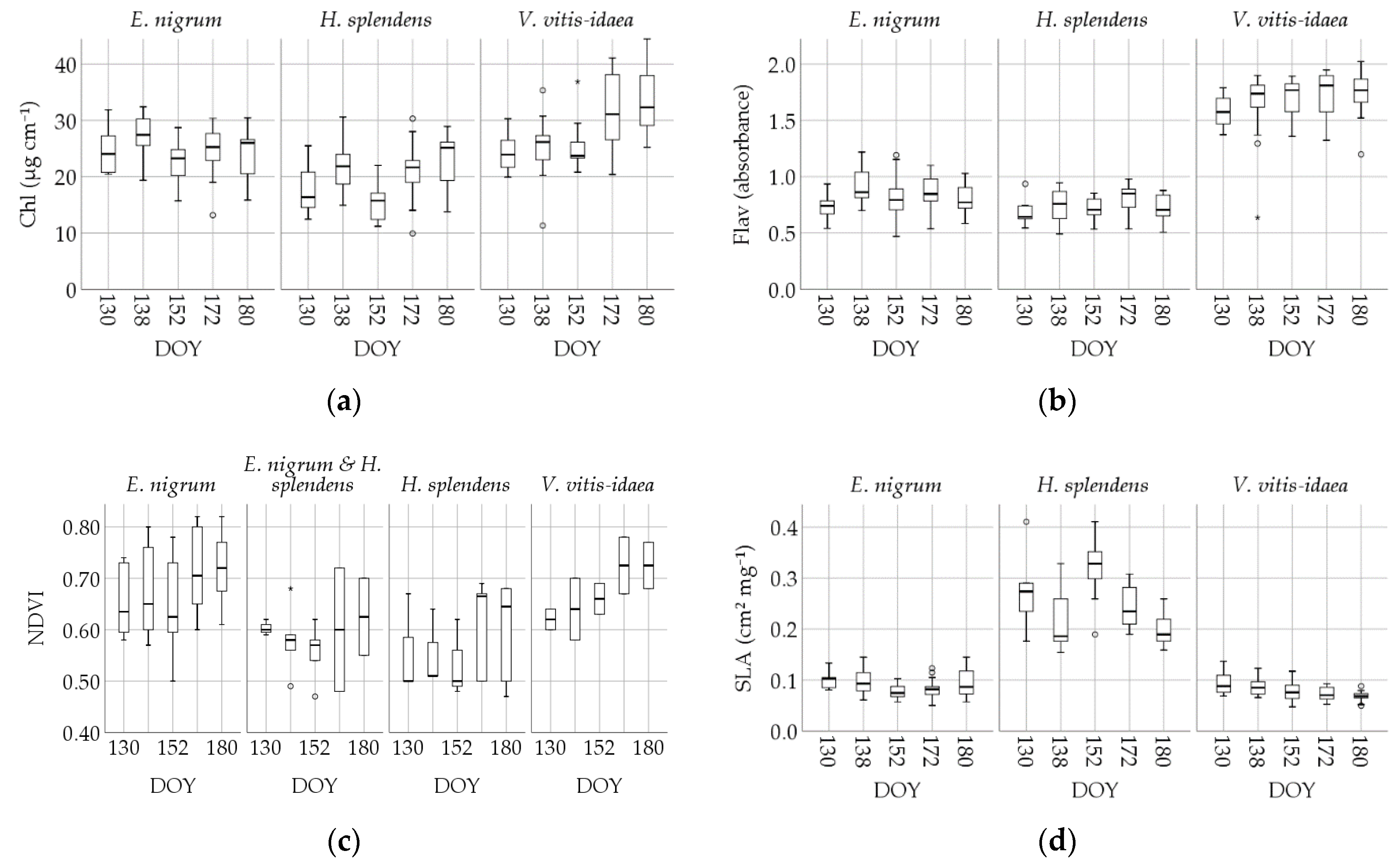
3.3. Intraspecific Trait Variablility

Table 5. Descriptive statistics of the monitored plant traits on species level.

Name	Specie	Mean	N	Std. Deviation	Std. Error	Median	5% PCTL	25% PCTL	75% PCTL	95% PCTL
Greenseeker NDVI	E. nigrum	0.65	59	0.094	0.012	0.62	0.49	0.58	0.72	0.82
	H. splendens	0.59	19	0.086	0.020	0.62	0.47	0.50	0.67	0.68 (90%)
	V. vitis-idaea	0.67	10	0.066	0.020	0.67	0.58	0.62	0.72	0.78 (90%)
Channel G%	E. nigrum	0.405	58	0.050	0.006	0.393	0.333	0.372	0.444	0.511
	H. splendens	0.396	19	0.037	0.008	0.383	0.350	0.383	0.415	0.474 (90%)
	V. vitis-idaea	0.397	10	0.046	0.015	0.389	0.355	0.363	0.408	0.497 (90%)
Plant height	E. nigrum	10.4	33	3.975	0.692	9.5	4,7	7.0	13.3	17.9
	H. splendens	5.5	11	1.955	0.589	5.0	3.5	4.0	6.5	9.7 (90%)
	V. vitis-idaea	11.8	6	6.55	2.676	10.5	6.0	6.0	19.0	-
SLA	E. nigrum	0.089	69	0.022	0.0027	0.085	0.057	0.072	0.105	0.130
	H. splendens	0.257	69	0.086	0.0104	0.246	0.164	0.189	0.291	0.411
	V. vitis-idaea	0.080	61	0.019	0.0024	0.079	0.052	0.066	0.092	0.117
Chl	E. nigrum	24.72	70	4.267	0.510	25.26	16.25	21.44	27.57	30.67
	H. splendens	19.88	69	5.122	0.617	20.01	11.90	15.59	23.88	28.54
	V. vitis-idaea	28.25	61	6.491	0.831	26.55	20.21	23.63	31.39	40.96
Flav	E. nigrum	0.833	69	0.164	0.020	0.818	0.542	0.727	0.943	1.145
	H. splendens	0.736	67	0.126	0.015	0.728	0.519	0.642	0.842	0.942
	V. vitis-idaea	1.671	61	0.232	0.030	1.706	1.297	1.558	1.843	1.944

illustrates the overall trait variability during the study. Plant traits varied in the course of the study, with species showing contrasting responses (Figure 3). For example, Chl increased in V. vitis-idaea, but was stable in E. nigrum and H. splendens (Figure 3a), while the flavonol content was rather constant over time, but significantly higher in V. vitis-idaea than in the other two species (Figure 3b). In early June, however, all studied species showed a sudden decline in chlorophyll content (Figure 3a; DOY 152), (F_4,14 = 7.945, p < 0.001), which coincided with the temperature dropping almost to freezing point and light snowfall during DOYs 150–151 (Figure S4). The post-hoc Bonferroni test confirms significant differences in chlorophyll content on the sampling dates before (DOY 138) and after (DOY 172) the temperature drop (p = 0.020 and p = 0.015). NDVI varied considerably within species (long boxes in Figure 3c) and only V. vitis-idaea showed a temporal trend in NDVI, which coincided with an increase in chlorophyll content (compare Figure 3a,c). SLA was constant over time, but significantly higher in the moss than in the two dwarf shrubs (Figure 3d).

3.4. Suitable Traits for Stress Monitoring

Our stress level estimate (Table 4) correlated with NDVI (r = −0.600, p < 0.001) and BNDVI (r = −0.654, p < 0.001), while the RGB indices performed best; r = 0.768, p < 0.001 for the Channel G% and r = −0.745, p < 0.001 for the GRVI, both as linear functions. Allowing a logistic relationship, a higher correlation level is obtained r = −0.833, p < 0.001 (Figure 4a) and r = −0.650, p < 0.001 (Figure 4b). Stress level estimates were also significantly correlated with plant height (r = −0.553, p = 0.001), as well as with soil depth (r = −0.336, p < 0.05). For litter, the relation with stress is reasonable, but not significant (r = −0.419, p = 0.084, n = 18). Neither flavonol absorbance nor chlorophyll content or the NBI readings could be related to the stress estimate (Table 4). No correlation was found for SLA and stress level (n = 14).

4. Discussion

The range of intraspecific trait variability (1^st research question), is attributed well during the study. Some plant traits remained relatively stable during spring (SLA, Plant height, Flav), while others showed more variations during the season and to environmental circumstances (NDVI, ChannelG% and Chl). The small leaves of E. nigrum and shoots of H. splendens made the SLA measurements challenging. However, the infrequently used method that we decided to apply seemed to work well, as our results are comparable to SLA values retrieved in previous studies [48,49,50]. To our knowledge, our plots did not suffer from any major stress (browning) events during the last 3 years prior to our measurements, except that Vaccinium myrtillus in the area had been partly defoliated by larvae of geometrid moths [51], but this species was rare or absent in our plots. In the early growing season, plants are especially vulnerable to winter-related stress and are showing accumulated stress responses from the previous years [13,14]. Hence, we monitored the natural range of trait variabilities from start of the growing season (DOY 130) onwards. Chlorophyll content was dropping significantly when temperature fell to almost freezing point. However, more research is needed to validate this result. It might be that the slight snowfall, or both parameters jointly, instigated the decline in chlorophyll concentrations.

The second research question was to assess whether any of the studied plant traits are suitable for stress monitoring. Our data show that the stress level differed between plots; we found that plant height was related to soil depth and that soil depth was also related to NBI. Although we did not find any significant correlation between plant height and NBI, we assume that soil depth is a limiting factor for this ecosystem. Lower soil depth affects water and nutrient availability as well as soil temperature [52] and is also associated with areas of low snow accumulation during winter [13]. This is supported by the fact that the stress level decreased with increasing soil depth and that NDVI increased with increasing soil depth.

In general, the flavonol content is associated with plant stress reactions [53]. However, we could not relate the flavonol absorbance to our stress level estimates. As the Dualex device estimates the flavonol content from spectral properties, it might not be able to measure the relevant flavonols in relation to the types of stress occurring in these subarctic plants. Dualex flavonol measurements are performed at the wavelengths 375 nm (UV-A) and 650 nm (red) [34]. This results in screening of mainly kaempferol, quercetin, and myricetin [53]. Our results are in agreement with Lefebvre et al. [54], who concluded that the Dualex device could not accurately predict the flavonol content in the three alpine plants they studied.

Concerning the third research question, our results show that ordinary RGB cameras may be used as NDVI surrogates and that they reflect various plant traits well. They performed equally well as modified cameras (with the infrared filter removed) for near-remote sensing approaches in the subarctic ecosystem. We found that a normal gray card, as used by professional photographers, was sufficient for the calibration process. Based on our findings, we recommend a simple white balance. Even if correlations to NDVI were slightly higher for BNDVI (r = 0.779) than for RGB greenness indices (0.689−0.749), one of the main strengths of the RGB cameras is that they are easier to operate than the modified devices. Sonnentag et al. [46] showed that different RGB cameras produce comparable results and that the choice of file format is not that important. Also, Nijland et al. [55] identified band separation and dynamic range as main problems when using converted cameras and therefore recommended the use of true color imaging. Another aspect is that the distribution of RGB cameras via smartphones is enormous and might be valuable for citizen science projects or app development [56]. In general, our greenness measurements are in agreement with existing reports on phenology at higher latitudes [30,57].

Moreover, the Channel G% index performed better than NDVI in characterizing some plant traits. This includes the stress level which showed a stronger correlation to Channel G% (linear: r = −0.768 vs. r = −0.600; logistic: r = −0.833 vs. r = −0.651) and NBI which showed a significant correlation (r = −0.354) to Channel G%, but not to NDVI. Consequently, the Channel G% index is of additional value for screening plant stress (2^nd research question). The significant correlation between RGB indices and chlorophyll meter readings (r = 0.38, p < 0.05) also implies that the RGB-based indices could be potential NDVI surrogates (see Table 4). In contrast to previous studies [28,29,58], our GNDVI data did not show any significant correlation with chlorophyll content or other plant traits. Correlations between chlorophyll and NDVI showed reasonable results [29], indicating that chlorophyll measurements are valid in spite of the untypical leaf structures of H. splendens and E. nigrum.

We found a high correlation between spaceborne NDVI and ground-sampled NDVI measured by the active Greenseeker device (maximum r = 0.968 for the Sentinel-2 NDVI calculated with bands 4 and 7). Nevertheless, despite of the strongly significant correlation, it is based only on 14 data points, implying that relationships have to be handled with care. It is a higher correlation than retrieved in previous studies, where near-remotely sensed NDVI data were compared to NDVI from Sentinel-2 and Landsat 8 [59,60]. A likely reason for the very strong correlation is that this study was carried out in a very open subarctic woodland (in parts nearly treeless and then considered as heath) where understory vegetation contributes very much to the NDVI detected by the satellites. We did not find major differences in the correlations, even when spectral properties (bandwidth and wavelength peaks) were not similar. This strongly suggests that active sensors can be used for validation of spaceborne data, for example, from Sentinel-2.

5. Conclusions

The objective of this study was to assess the applicability of common plant traits and near-remote sensing approaches as tools to monitor the health state of dominant understory subarctic vegetation types that previously were shown to be vulnerable to winter climate change and other types of stress. In order to determine intraspecific trait variability, species were monitored in different health states. Due to this screening we are able to better validate the effect size of a browning event on the studied species. As the study was set in an area not recently damaged by stressful events, the different stress levels could be explained by differences in soil depth, which again act as a surrogate for several potential stressful elements, including moisture and nutrient deficits during the growing season and little snow protection during winter. Channel G% was the best RGB-based index in our study, and we recommend the use of this index. Finally, we found promising results by combining spaceborne Sentinel-2 data with the active near-remote sensor for measurements of NDVI. This could be a useful tool for upscaling the role of understory vegetation to the total NDVI measured by satellites in regions where browning occurs. Further research is recommended on the satellite upscaling, but also on the measured chlorophyll drop following a rapid midsummer temperature decrease to freezing point. Finally, we recommend following the same plots after a stressful weather event, to report direct as well as long-term changes in situ.

References

1. Pachauri, R.K.; Allen, M.R.; Barros, V.R.; Broome, J.; Cramer, W.; Christ, R.; Church, J.A.; Clarke, L.; Dahe, Q.; Dasgupta, P.; et al. Climate Change 2014: Synthesis Report; Pachauri, R.K., Mayer, L., Eds.; Intergovernmental Panel on Climate Change: Geneva, Switzerland, 2015. [Google Scholar]
2. Ju, J.; Masek, J.G. The vegetation greenness trend in Canada and US Alaska from 1984–2012 Landsat data. Remote Sens. Environ. 2016, 176, 1–16. [Google Scholar] [CrossRef]
3. Myneni, R.B.; Keeling, C.D.; Tucker, C.J.; Asrar, G.; Nemani, R.R. Increased plant growth in the northern high latitudes from 1981 to 1991. Nature 1997, 386, 698–702. [Google Scholar] [CrossRef]
4. Verbyla, D. The greening and browning of Alaska based on 1982–2003 satellite data. Glob. Ecol. Biogeogr. 2008, 17, 547–555. [Google Scholar] [CrossRef]
5. Jia, G.J.; Epstein, H.E.; Walker, D.A. Greening of arctic Alaska, 1981–2001. Geophys. Res. Lett. 2003, 30. [Google Scholar] [CrossRef]
6. Epstein, H.E.; Bhatt, U.S.; Raynolds, M.K.; Walker, D.A.; Forbes, B.C.; Phoenix, G.K.; Bjerke, J.W.; Tømmervik, H.; Karlsen, S.-R.; Myneni, R.; et al. Tundra greenness. Bull. Am. Meteorol. Soc. 2019, 100, S163–S168. [Google Scholar]
7. Myers-Smith, I.H.; Kerby, J.T.; Phoenix, G.K.; Bjerke, J.W.; Epstein, H.E.; Assmann, J.J.; John, C.; Andreu-Hayles, L.; Angers-Blondin, S.; Beck, P.S.A.; et al. Complexity revealed in the greening of the Arctic. Nat. Clim. Chang. 2020, 10, 106–117. [Google Scholar] [CrossRef] [Green Version]
8. Phoenix, G.K.; Bjerke, J.W. Arctic browning: Extreme events and trends reversing arctic greening. Glob. Chang. Biol. 2016, 22, 2960–2962. [Google Scholar] [CrossRef]
9. Bokhorst, S.F.; Bjerke, J.W.; Bowles, F.W.; MELILLO, J.; Callaghan, T.V.; Phoenix, G.K. Impacts of extreme winter warming in the sub-Arctic: Growing season responses of dwarf shrub heathland. Glob. Chang. Biol. 2008, 14, 2603–2612. [Google Scholar] [CrossRef]
10. Sorensen, P.O.; Finzi, A.C.; Giasson, M.A.; Reinmann, A.B.; Sanders-DeMott, R.; Templer, P.H. Winter soil freeze-thaw cycles lead to reductions in soil microbial biomass and activity not compensated for by soil warming. Soil. Biol. Biochem. 2018, 116, 39–47. [Google Scholar] [CrossRef] [Green Version]
11. Bokhorst, S.F.; Bjerke, J.W.; Street, L.E.; Callaghan, T.V.; Phoenix, G.K. Impacts of multiple extreme winter warming events on sub-Arctic heathland: Phenology, reproduction, growth, and CO2 flux responses. Glob. Chang. Biol. 2011, 17, 2817–2830. [Google Scholar] [CrossRef]
12. Bokhorst, S.F.; Phoenix, G.K.; Berg, M.P.; Callaghan, T.V.; Kirby-Lambert, C.; Bjerke, J.W. Climatic and biotic extreme events moderate long-term responses of above- and belowground sub-Arctic heathland communities to climate change. Glob. Chang. Biol. 2015, 21, 4063–4075. [Google Scholar] [CrossRef] [PubMed] [Green Version]
13. Bjerke, J.W.; Treharne, R.; Vikhamar-Schuler, D.; Karlsen, S.R.; Ravolainen, V.; Bokhorst, S.F.; Phoenix, G.K.; Bochenek, Z.; Tømmervik, H. Understanding the drivers of extensive plant damage in boreal and Arctic ecosystems: Insights from field surveys in the aftermath of damage. Sci. Total Environ. 2017, 599, 1965–1976. [Google Scholar] [CrossRef] [PubMed]
14. Bjerke, J.W.; Bokhorst, S.F.; Callaghan, T.V.; Phoenix, G.K.; Dorrepaal, E. Persistent reduction of segment growth and photosynthesis in a widespread and important sub-Arctic moss species after cessation of three years of experimental winter warming. Funct. Ecol. 2017, 31, 127–134. [Google Scholar] [CrossRef] [Green Version]
15. Bjerke, J.W.; Rune Karlsen, S.; Arild Høgda, K.; Malnes, E.; Jepsen, J.U.; Lovibond, S.; Vikhamar-Schuler, D.; Tømmervik, H. Record-low primary productivity and high plant damage in the Nordic Arctic Region in 2012 caused by multiple weather events and pest outbreaks. Environ. Res. Lett. 2014, 9, 84006. [Google Scholar] [CrossRef]
16. Tømmervik, H.; Bjerke, J.W.; Park, T.; Hanssen, F.; Myneni, R.B. Legacies of historical exploitation of natural resources are more important than summer warming for recent biomass increases in a boreal–Arctic transition region. Ecosystems 2019, 113, 11770. [Google Scholar] [CrossRef]
17. Xu, L.; Myneni, R.B.; Chapin III, F.S.; Callaghan, T.V.; Pinzon, J.E.; Tucker, C.J.; Zhu, Z.; Bi, J.; Ciais, P.; Tømmervik, H.; et al. Temperature and vegetation seasonality diminishment over northern lands. Nat. Clim. Chang. 2013. [Google Scholar] [CrossRef] [Green Version]
18. Kitić, G.; Tagarakis, A.; Cselyuszka, N.; Panić, M.; Birgermajer, S.; Sakulski, D.; Matović, J. A new low-cost portable multispectral optical device for precise plant status assessment. Comput. Electron. Agric. 2019, 162, 300–308. [Google Scholar] [CrossRef]
19. Bokhorst, S.F.; Tømmervik, H.; Callaghan, T.V.; Phoenix, G.K.; Bjerke, J.W. Vegetation recovery following extreme winter warming events in the sub-Arctic estimated using NDVI from remote sensing and handheld passive proximal sensors. Environ. Exp. Bot. 2012, 81, 18–25. [Google Scholar] [CrossRef]
20. Street, L.E.; Shaver G., R.; Williams, M.; Van Wijk, M.T. What is the relationship between changes in canopy leaf area and changes in photosynthetic CO 2 flux in arctic ecosystems? J. Ecol. 2007, 95, 139–150. [Google Scholar] [CrossRef]
21. Rouse, J.; Haas, H.R.; Schell, A.J.; Deering, W.D. Monitoring vegetation systems in the Great Plains with ERTS. In Proceedings of the 3rd Earth Resource Technology Satellite-1 Symposium, Washington, DC, USA, 10–14 December 1973. [Google Scholar]
22. Tucker, C.J. Red and photographic infrared linear combinations for monitoring vegetation. Remote Sens. Environ. 1979, 8, 127–150. [Google Scholar] [CrossRef] [Green Version]
23. Pettorelli, N.; Vik, J.O.; Mysterud, A.; Gaillard, J.-M.; Tucker, C.J.; Stenseth, N.C. Using the satellite-derived NDVI to assess ecological responses to environmental change. Trends Ecol. Evol. 2005, 20, 503–510. [Google Scholar] [CrossRef] [PubMed]
24. Boelman, N.T.; Stieglitz, M.; Rueth, H.M.; Sommerkorn, M.; Griffin, K.L.; Shaver, G.R.; Gamon, J.A. Response of NDVI, biomass, and ecosystem gas exchange to long-term warming and fertilization in wet sedge tundra. Oecologia 2003, 135, 414–421. [Google Scholar] [CrossRef] [PubMed]
25. Jepsen, J.U.; Hagen, S.B.; Høgda, K.A.; Ims, R.A.; Karlsen, S.R.; Tømmervik, H.; Yoccoz, N.G. Monitoring the spatio-temporal dynamics of geometrid moth outbreaks in birch forest using MODIS-NDVI data. Remote Sens. Environ. 2009, 113, 1939–1947. [Google Scholar] [CrossRef]
26. Tømmervik, H.; Karlsen, S.-R.; Nilsen, L.; Johansen, B.; Storvold, R.; Zmarz, A.; Becker, P.S.; Johansen, K.-S.; Hogda, K.-A.; Goetz, S.; et al. Use of Unmanned Aircraft Systems (UAS) in a Multi-Scale Vegetation Index Study of Arctic Plant Communities in Adventdalen on Svalbard. Available online: https://www.nina.no/Portals/NINA/Bilder%20og%20dokumenter/Prosjekter/ArcticBiomass/Tommervik_et_2014_UAS_RPAS.pdf (accessed on 26 January 2020).
27. Leblanc, S.G.; Chen, W.; Maloley, M.; Humphreys, E.; Elliott, C. NDVI Digital Camera for Monitoring Arctic Vegetation. In Proceedings of the 2014 IEEE International Geoscience & Remote Sensing Symposium and 35th Canadian Symposium on Remote Sensing (IGARSS 2014/35th CSRS), Quebec, Canada, 13–18 July 2014. [Google Scholar]
28. Gitelson, A.A.; Merzlyak, M.N. Remote estimation of chlorophyll content in higher plant leaves. Int. J. Remote Sens. 1997, 18, 2691–2697. [Google Scholar] [CrossRef]
29. Hunt, E.R.; Doraiswamy, P.C.; McMurtrey, J.E.; Daughtry, C.S.T.; Perry, E.M.; Akhmedov, B. A visible band index for remote sensing leaf chlorophyll content at the canopy scale. Int. J. Appl. Earth Obs. Geoinf. 2013, 21, 103–112. [Google Scholar] [CrossRef] [Green Version]
30. Anderson, H.; Nilsen, L.; Tømmervik, H.; Karlsen, S.; Nagai, S.; Cooper, E.J. Using Ordinary Digital Cameras in Place of Near-Infrared Sensors to Derive Vegetation Indices for Phenology Studies of High Arctic Vegetation. Remote Sens. 2016, 8, 847. [Google Scholar] [CrossRef] [Green Version]
31. Nilsson, M.-C.; Wardle, D.A. Understory vegetation as a forest ecosystem driver: Evidence from the northern Swedish boreal forest. Front Ecol. Environ. 2005, 3. [Google Scholar] [CrossRef]
32. Lomolino, M.V.; Riddle, B.R.; Whittaker, R.J.; Brown, J.H. Biogeography, 4th ed.; Sinauer: Sunderland, MA, USA, 2010; p. 662. [Google Scholar]
33. Bjerke, J.W.; Bokhorst, S.F.; Zielke, M.; Callaghan, T.V.; Bowles, F.W.; Phoenix, G.K. Contrasting sensitivity to extreme winter warming events of dominant sub-Arctic heathland bryophyte and lichen species. J. Ecol. 2011, 99, 1481–1488. [Google Scholar] [CrossRef]
34. Cerovic, Z.G.; Masdoumier, G.; Ghozlen, N.B.; Latouche, G. A new optical leaf-clip meter for simultaneous non-destructive assessment of leaf chlorophyll and epidermal flavonoids. Physiol. Plant 2012, 146, 251–260. [Google Scholar] [CrossRef]
35. Cartelat, A.; Cerovic, Z.G.; Goulas, Y.; Meyer, S.; Lelarge, C.; Prioul, J.-L.; Barbottin, A.; Jeuffroy, M.-H.; Gate, P.; Agati, G.; et al. Optically assessed contents of leaf polyphenolics and chlorophyll as indicators of nitrogen deficiency in wheat (Triticum aestivum L.). Field Crops Res. 2005, 91, 35–49. [Google Scholar] [CrossRef]
36. Palta, J.P. Leaf chlorophyll content. Remote Sensing Reviews 1990, 5, 207–213. [Google Scholar] [CrossRef]
37. Pierce, L.L.; Running, S.W.; Walker, J. Regional-Scale Relationships of Leaf Area Index to Specific Leaf Area and Leaf Nitrogen Content. Ecol. Appl. 1994, 4, 313–321. [Google Scholar] [CrossRef] [Green Version]
38. Liu, M.; Wang, Z.; Li, S.; Lü, X.; Wang, X.; Han, X. Changes in specific leaf area of dominant plants in temperate grasslands along a 2500-km transect in northern China. Sci. Rep. 2017, 7, 10780. [Google Scholar] [CrossRef] [PubMed]
39. Cornelissen, J.H.C.; Lavorel, S.; Garnier, E.; Díaz, S.; Buchmann, N.; Gurvich, D.E.; Reich, P.B.; Steege, H.t.; Morgan, H.D.; Van der Heijden, M.G.A.; et al. A handbook of protocols for standardised and easy measurement of plant functional traits worldwide. Aust. J. Bot. 2003, 51, 335. [Google Scholar] [CrossRef] [Green Version]
40. Treharne, R.; Bjerke, J.W.; Tømmervik, H.; Stendardi, L.; Phoenix, G.K. Arctic browning: Impacts of extreme climatic events on heathland ecosystem CO2 fluxes. Glob. Chang. Biol. 2019, 25, 489–503. [Google Scholar] [CrossRef] [PubMed] [Green Version]
41. Martin, D.; López, J.; Lan, Y. Laboratory evaluation of the GreenSeeker™ hand-held optical sensor to variations in orientation and height above canopy. Int. J. Agric. Biol. Eng. 2012, 43–47. [Google Scholar] [CrossRef]
42. Verhulst, N.; Govaerts, B.; Sayre, K.D.; Deckers, J.; François, I.M.; Dendooven, L. Using NDVI and soil quality analysis to assess influence of agronomic management on within-plot spatial variability and factors limiting production. Plant Soil. 2009, 317, 41–59. [Google Scholar] [CrossRef]
43. Koucká, L.; Kopačková, V.; Fárová, K.; Gojda, M. UAV Mapping of an Archaeological Site Using RGB and NIR High-Resolution Data. Proceedings 2018, 2, 351. [Google Scholar] [CrossRef] [Green Version]
44. MaxMax. Manufacturer Homepage; Product Specifications. Available online: https://maxmax.com/ndvi_camera_technical.htm (accessed on 6 September 2017).
45. Bannari, A.; Morin, D.; Bonn, F.; Huete, A.R. A review of vegetation indices. Remote Sensing Reviews 1995, 13, 95–120. [Google Scholar] [CrossRef]
46. Sonnentag, O.; Hufkens, K.; Teshera-Sterne, C.; Young, A.M.; Friedl, M.; Braswell, B.H.; Milliman, T.; O’Keefe, J.; Richardson, A.D. Digital repeat photography for phenological research in forest ecosystems. Agric. For. Meteorol. 2012, 152, 159–177. [Google Scholar] [CrossRef]
47. Richardson, A.D.; Jenkins, J.P.; Braswell, B.H.; Hollinger, D.Y.; Ollinger, S.V.; Smith, M.-L. Use of digital webcam images to track spring green-up in a deciduous broadleaf forest. Oecologia 2007, 152, 323–334. [Google Scholar] [CrossRef] [PubMed]
48. Suzuki, S.; Kudo, G. Short-term effects of simulated environmental change on phenology, leaf traits, and shoot growth of alpine plants on a temperate mountain, northern Japan. Glob. Chang. Biol. 1997, 3, 108–115. [Google Scholar] [CrossRef]
49. Pensa, M.; Karu, H.; Luud, A.; Kund, K. Within-species correlations in leaf traits of three boreal plant species along a latitudinal gradient. Plant Ecol. 2010, 208, 155–166. [Google Scholar] [CrossRef]
50. Van Wijk, M.T.; Williams, M.; Shaver, G.R. Tight coupling between leaf area index and foliage N content in arctic plant communities. Oecologia 2005, 142, 421–427. [Google Scholar] [CrossRef] [PubMed] [Green Version]
51. Bjerke, J.W.; Wierzbinski, G.; Tømmervik, H.; Phoenix, G.K.; Bokhorst, S. Stress-induced secondary leaves of a boreal deciduous shrub (Vaccinium myrtillus) overwinter then regain activity the following growing season. Nord. J. Bot. 2018, 36, e01894. [Google Scholar] [CrossRef]
52. Tybirk, K.; Nilsson, M.-C.; Michelsen, A.; Kristensen, H.L.; Shevtsova, A.; Strandberg, M.T.; Johansson, M.; Nielsen, K.E.; Riis-Nielsen, T.; Strandberg, B.; et al. Nordic Empetrum dominated ecosystems: Function and susceptibility to environmental changes. Ambio 2000, 29, 90–97. [Google Scholar] [CrossRef]
53. Cerovic, Z.G.; Ounis, A.; Cartelat, A.; Latouche, G.; Goulas, Y.; Meyer, S.; Moya, I. The use of chlorophyll fluorescence excitation spectra for the non-destructive in situ assessment of UV-absorbing compounds in leaves. Plant Cell Environ. 2002, 25, 1663–1676. [Google Scholar] [CrossRef]
54. Lefebvre, T.; Millery-Vigues, A.; Gallet, C. Does leaf optical absorbance reflect the polyphenol content of alpine plants along an elevational gradient? Alp. Bot. 2016, 126, 177–185. [Google Scholar] [CrossRef]
55. Nijland, W.; De Jong, R.; De Jong, S.M.; Wulder, M.A.; Bater, C.W.; Coops, N.C. Monitoring plant condition and phenology using infrared sensitive consumer grade digital cameras. Agric. For. Meteorol. 2014, 184, 98–106. [Google Scholar] [CrossRef] [Green Version]
56. Leeuw, T.; Boss, E. The HydroColor app: Above water measurements of remote sensing reflectance and turbidity using a smartphone camera. Sensors 2018, 18, 256. [Google Scholar] [CrossRef] [Green Version]
57. Westergaard-Nielsen, A.; Lund, M.; Hansen, B.U.; Tamstorf, M.P. Camera derived vegetation greenness index as proxy for gross primary production in a low Arctic wetland area. ISPRS Int. J. Geoinf. 2013, 86, 89–99. [Google Scholar] [CrossRef]
58. Hunt, E.R.; Hively, W.D.; McCarty, G.W.; Daughtry, C.S.T.; Forrestal, P.J.; Kratochvil, R.J.; Carr, J.L.; Allen, N.F.; Fox-Rabinovitz, J.R.; Miller, C.D. NIR-Green-Blue High-Resolution Digital Images for Assessment of Winter Cover Crop Biomass. GIScience Remote Sens. 2011, 48, 86–98. [Google Scholar]
59. Manna, S.; Raychaudhuri, B. Retrieval of leaf area index and stress conditions for Sundarban mangroves using Sentinel-2 data. Int. J. Remote Sens. 2019, 1–21. [Google Scholar] [CrossRef]
60. Barbanti, L.; Adroher, J.; Damian, J.M.; Di Virgilio, N.; Falsone, G.; Zucchelli, M.; Martelli, R. Assessing wheat spatial variation based on proximal and remote spectral vegetation indices and soil properties. Ital. J. Agronomy 2018, 13, 21. [Google Scholar] [CrossRef] [Green Version]
Figure 1. Species are marked with different symbols (see legend). 95% confidence intervals are grey. All correlations are significant (p < 0.001). The panels show the relationships between: (a) The active Greenseeker and the passive Mapir NDVI; (b) the BNDVI from the modified camera and NDVI; (c) Channel G% from the ordinary camera and NDVI; (d) chlorophyll content (Chl) and NDVI; (e) and (f) represent our satellite upscaling; comparing ground-based Greenseeker NDVI and Sentinel-2 NDVI, (note n = 14). NDVI is calculated with the named bands (= B). Equations and RMSE are shown in Table S4.
Sensors 20 02102 g001
Figure 2. Relationship of two trait correlations from Table 4. Species are marked. 95% confidence intervals are grey. Relation between (a) median plant height and NDVI, (b) chlorophyll content and SLA. Equations and RMSE are shown in Table S4.
Sensors 20 02102 g002
Figure 3. Intraspecific trait variability and its changes during the spring season for the species Empterum nigrum, Vaccinium vitis-idaea, and Hylocomium splendens. All species were monitored in varying health states, while each value represents one plot dominated by the named species. (a) Chlorophyll content (Chl); (b) flavonols (Flav); relative absorbance values; (c) Greenseeker NDVI; (d) SLA. These results were obtained at a moisture content (percent of wet weight) ranging from 55% to 75% for H. splendens, 63 to 68% for V. vitis-idaea, and 63 to 71% for E. nigrum.
Sensors 20 02102 g003
Figure 4. Comparison of stress level to greenness indices. 95% confidence intervals are dashed. Relation between (a) stress level and the RGB index Channel G%; (b) stress level and Greenseeker NDVI. Equations are shown in Table S4.
Sensors 20 02102 g004