A Review of Visual-LiDAR Fusion based Simultaneous Localization and Mapping


Abstract
1. Introduction
2. Simultaneous Localization and Mapping
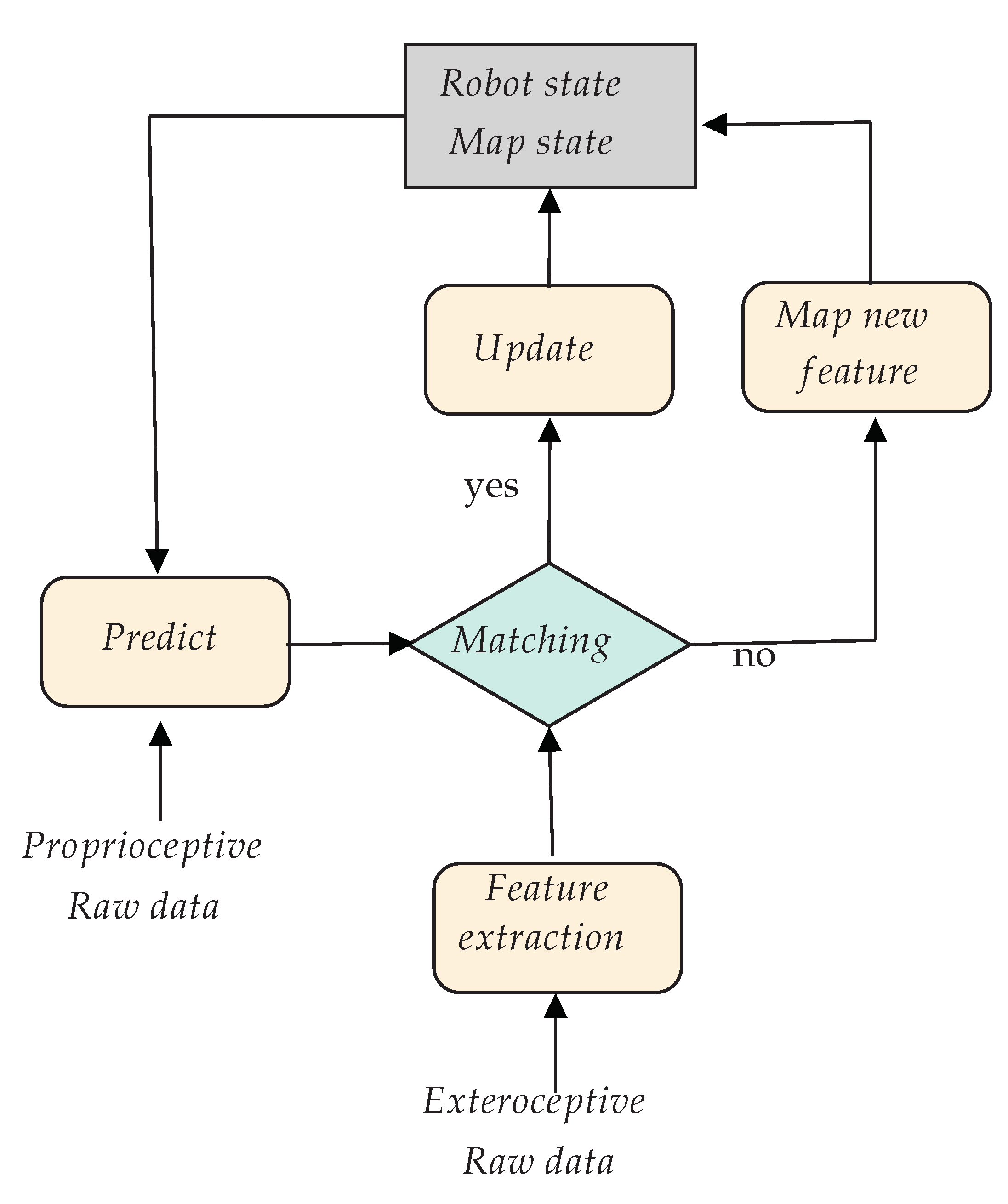
2.1. Principle
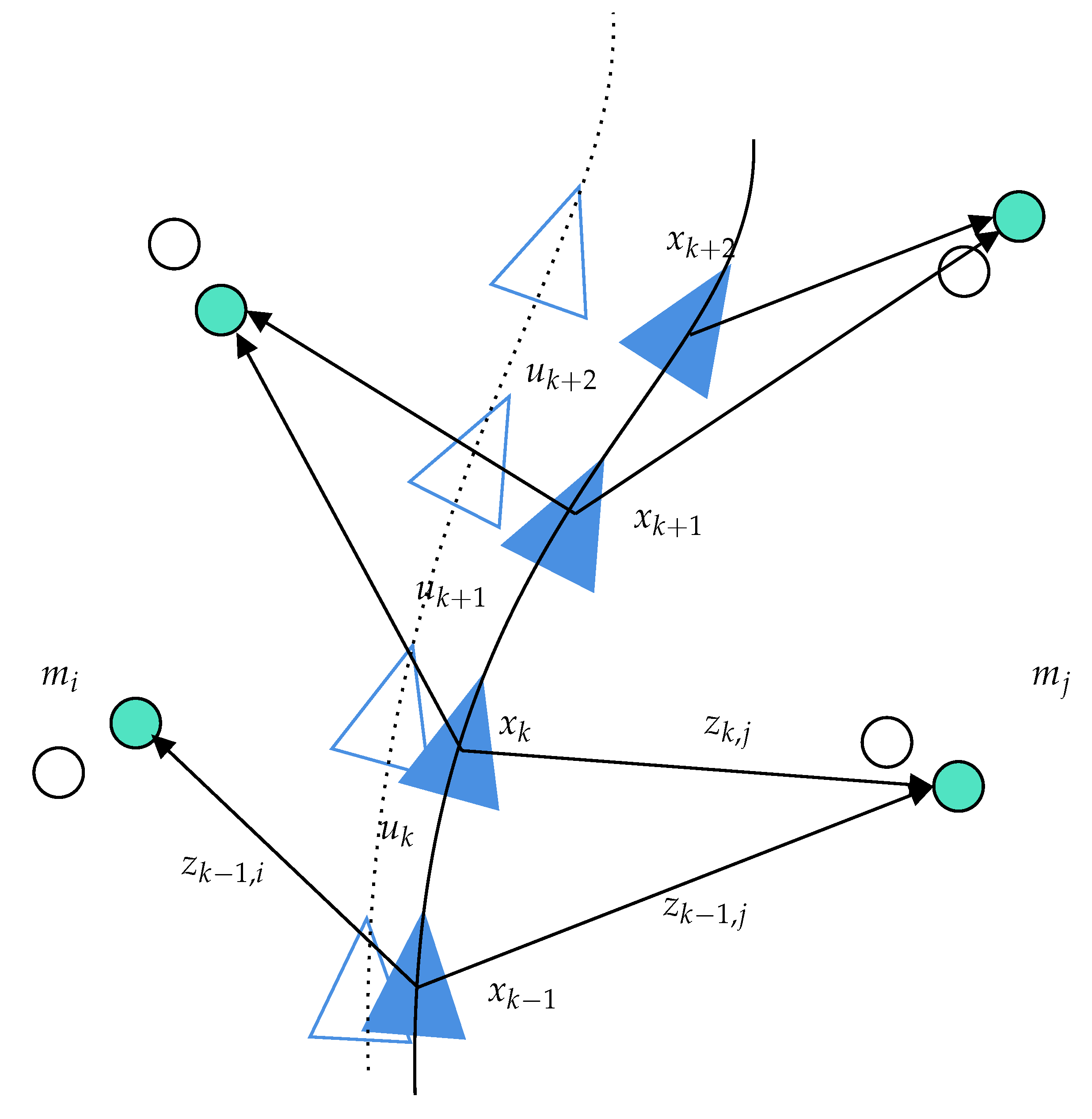
2.2. Probabilistic Solution of the SLAM Framework
- : the state vector describing the robot at time k
- : the estimated state vector at time k given the knowledge of the previous state
- : the control vector applied at to move the vehicle to a state (if provided)
- : a vector describing the landmark
- : an observation of the landmark taken at time k
- X: the set of vehicle locations from Time 0 to k
- : the set of control inputs from Time 0 to k
- : the set of observations from Time 0 to k
- M: the set of landmarks or maps
- : the estimated map at time k given the knowledge of the previous map at time .
2.3. Graph Based Solution of the SLAM Framework
3. Visual-SLAM
3.1. Feature Based SLAM
3.2. Direct SLAM
3.3. RGB-D SLAM
3.4. Event Camera SLAM
3.5. Visual SLAM Conclusions
4. LiDAR Based SLAM
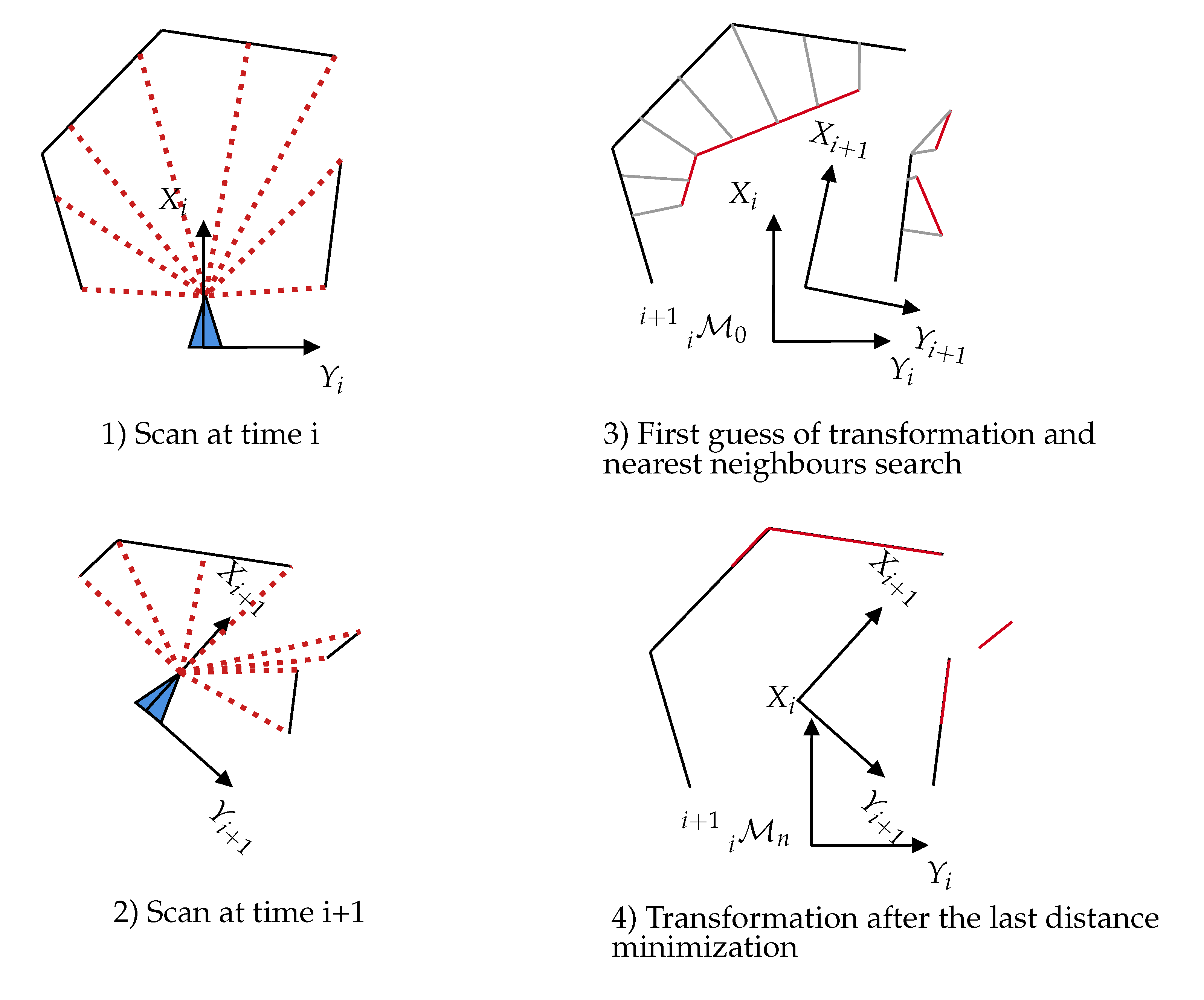
4.1. Scan-Matching and Graph Optimization
4.1.1. Occupancy Map and Particle Filter
4.1.2. Loop Closure Refinement Step
5. LiDAR-Camera Fusion
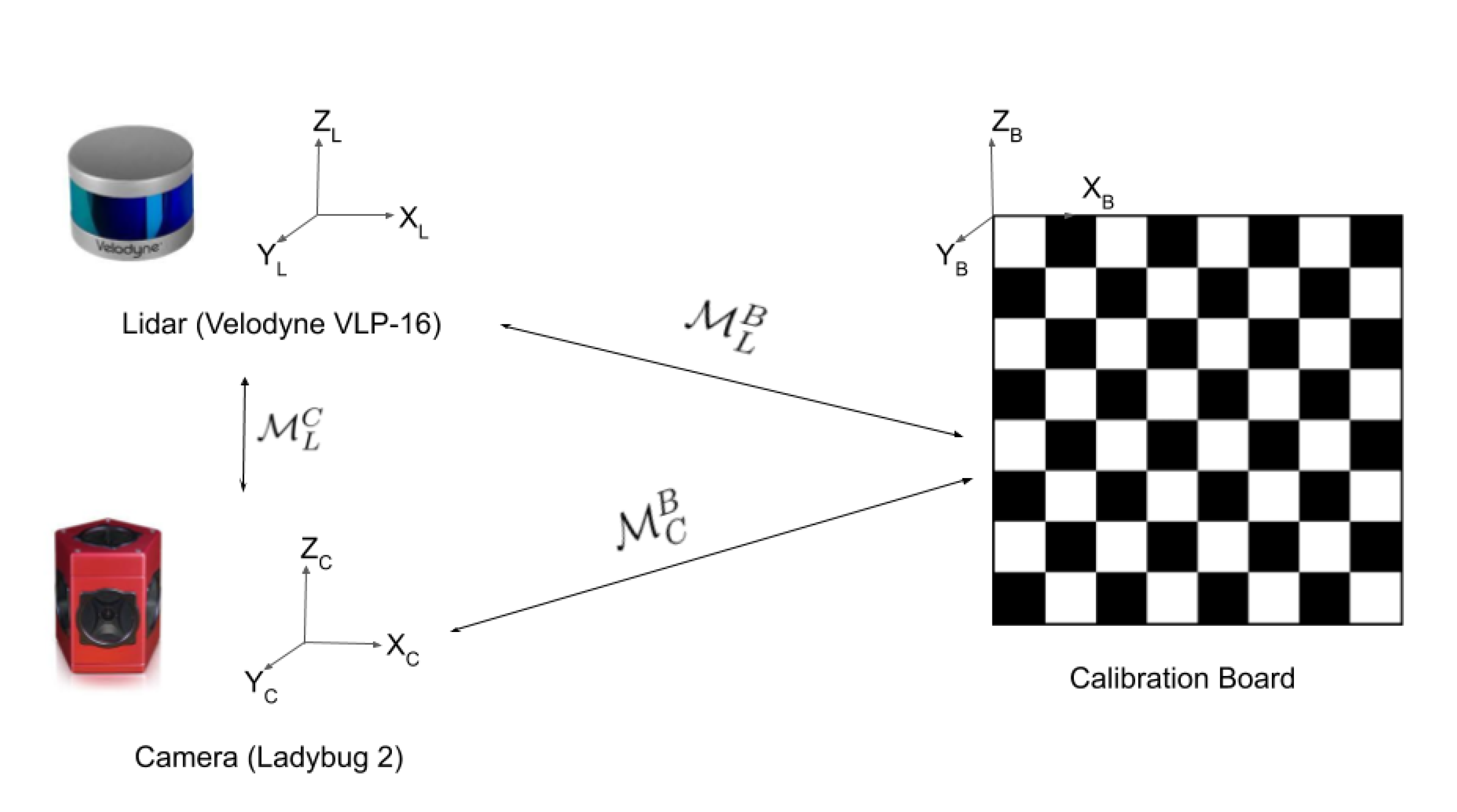
5.1. The Mandatory Calibration Step
5.2. Visual-LiDAR SLAM
5.2.1. EKF Hybridized SLAM
5.2.2. Improved Visual SLAM
5.2.3. Improved LiDAR SLAM
5.2.4. Concurrent LiDAR-Visual SLAM
5.3. Summary
6. Discussion on Future Research Directions
7. Conclusions
Funding
Conflicts of Interest
References
- Dikmen, M.; Burns, C.M. Autonomous driving in the real world: Experiences with tesla autopilot and summon. In Proceedings of the 8th International Conference on Automotive User Interfaces and Interactive Vehicular Applications, Ann Arbor, MI, USA, 24–26 October 2016; pp. 225–228. [Google Scholar] [CrossRef]
- Gomes, L. When will Google’s self-driving car really be ready? It depends on where you live and what you mean by “ready”. IEEE Spectrum 2016, 53, 13–14. [Google Scholar] [CrossRef]
- Boersma, R.; Van Arem, B.; Rieck, F. Application of driverless electric automated shuttles for public transport in villages: The case of Appelscha. World Electric Veh. J. 2018, 9, 15. [Google Scholar] [CrossRef]
- Frese, U. A Discussion of Simultaneous Localization and Mapping. Auton. Robots 2006, 20, 25–42. [Google Scholar] [CrossRef]
- Chatila, R.; Laumond, J.P. Position referencing and consistent world modeling for mobile robots. In Proceedings of the 1985 IEEE International Conference on Robotics and Automation, St. Louis, MO, USA, 25–28 March 1985; Volume 2, pp. 138–145. [Google Scholar]
- Durrant-Whyte, H.; Bailey, T. Simultaneous localization and mapping: Part I. IEEE Robot. Autom. Mag. 2006, 13, 99–110. [Google Scholar] [CrossRef]
- Leonard, J.J.; Durrant-Whyte, H.F. Mobile robot localization by tracking geometric beacons. IEEE Trans. Robot. Autom. 1991, 7, 376–382. [Google Scholar] [CrossRef]
- Bustos, A.P.; Chin, T.J.; Eriksson, A.; Reid, I. Visual SLAM: Why Bundle Adjust? arXiv 2019, arXiv:1902.03747. [Google Scholar]
- Tateno, K.; Tombari, F.; Laina, I.; Navab, N. Cnn-slam: Real-time dense monocular slam with learned depth prediction. In Proceedings of the IEEE Conference on Computer Vision and Pattern Recognition, Honolulu, HI, USA, 22–25 July 2017; pp. 6243–6252. [Google Scholar]
- O’Mahony, N.; Campbell, S.; Krpalkova, L.; Riordan, D.; Walsh, J.; Murphy, A.; Ryan, C. Deep Learning for Visual Navigation of Unmanned Ground Vehicles: A review. In Proceedings of the 2018 29th Irish Signals and Systems Conference (ISSC), Belfast, Irland, 21–22 June 2018; pp. 1–6. [Google Scholar] [CrossRef]
- Koide, K.; Miura, J.; Menegatti, E. A portable three-dimensional LIDAR-based system for long-term and wide-area people behavior measurement. Int. J. Adv. Robotic Syst. 2019, 16, 1729881419841532. [Google Scholar] [CrossRef]
- Lu, F.; Milios, E. Globally consistent range scan alignment for environment mapping. Auton. Robots 1997, 4, 333–349. [Google Scholar] [CrossRef]
- Grisetti, G.; Kummerle, R.; Stachniss, C.; Burgard, W. A tutorial on graph-based SLAM. IEEE Intell. Trans. Syst. Mag. 2010, 2, 31–43. [Google Scholar] [CrossRef]
- Strasdat, H.; Montiel, J.M.M.; Davison, A.J. Visual SLAM: Why filter? Image Vis. Comput. 2012, 30, 65–77. [Google Scholar] [CrossRef]
- Davison, A.J.; Reid, I.D.; Molton, N.; Stasse, O. MonoSLAM: Real-Time Single Camera SLAM. IEEE Trans. Pattern Anal. Mach. Intell. 2007, 29, 1052–1067. [Google Scholar] [CrossRef] [PubMed]
- Davison, A.J. Real-Time Simultaneous Localisation and Mapping with a Single Camera. In Proceedings of the Ninth IEEE International Conference on Computer Vision, Nice, France, 13–16 October 2003; Volume 2, pp. 1403–1410. [Google Scholar]
- Klein, G.; Murray, D. Parallel Tracking and Mapping for Small AR Workspaces. In Proceedings of the 2007 6th IEEE and ACM International Symposium on Mixed and Augmented Reality, Nara, Japan, 13–16 November 2007; pp. 225–234. [Google Scholar] [CrossRef]
- Castle, R.; Klein, G.; Murray, D.W. Video-rate localization in multiple maps for wearable augmented reality. In Proceedings of the 2008 12th IEEE International Symposium on Wearable Computers, Pittsburgh, PA, USA, 28 September–1 October 2008; pp. 15–22. [Google Scholar]
- Pradeep, V.; Rhemann, C.; Izadi, S.; Zach, C.; Bleyer, M.; Bathiche, S. MonoFusion: Real-time 3D reconstruction of small scenes with a single web camera. In Proceedings of the 2013 IEEE International Symposium on Mixed and Augmented Reality (ISMAR), Adelaide, Australia, 1–4 October 2013; pp. 83–88. [Google Scholar]
- Mei, C.; Sibley, G.; Cummins, M.; Newman, P.M.; Reid, I.D. A Constant-Time Efficient Stereo SLAM System. In Proceedings of the British Machine Vision Conference, BMVC 2009, London, UK, 7–10 September 2009; pp. 1–11. [Google Scholar]
- Cummins, M.; Newman, P. FAB-MAP: Probabilistic localization and mapping in the space of appearance. Int. J. Robot. Res. 2008, 27, 647–665. [Google Scholar] [CrossRef]
- Mur-Artal, R.; Montiel, J.M.M.; Tardos, J.D. ORB-SLAM: A versatile and accurate monocular SLAM system. IEEE Trans. Robot. 2015, 31, 1147–1163. [Google Scholar] [CrossRef]
- Mur-Artal, R.; Tardós, J.D. Orb-slam2: An open-source slam system for monocular, stereo, and rgb-d cameras. IEEE Trans. Robot. 2017, 33, 1255–1262. [Google Scholar] [CrossRef]
- Vivet, D.; Debord, A.; Pagès, G. PAVO: A Parallax based Bi-Monocular VO Approach For Autonomous Navigation In Various Environments. In Proceedings of the DISP Conference, St Hugh College, Oxford, UK, 29–30 April 2019. [Google Scholar]
- Newcombe, R.A.; Lovegrove, S.J.; Davison, A.J. DTAM: Dense tracking and mapping in real-time. In Proceedings of the 2011 International Conference on Computer Vision, Barcelona, Spain, 6–13 November 2011; pp. 2320–2327. [Google Scholar]
- Engel, J.; Schöps, T.; Cremers, D. LSD-SLAM: Large-scale direct monocular SLAM. In Proceedings of the European Conference on Computer Vision, Zurich, Switzerland, 6–12 September 2014; pp. 834–849. [Google Scholar]
- Forster, C.; Pizzoli, M.; Scaramuzza, D. SVO: Fast semi-direct monocular visual odometry. In Proceedings of the 2014 IEEE International Conference on Robotics and Automation (ICRA), Hong Kong, China, 31 May–7 June 2014; pp. 15–22. [Google Scholar]
- Engel, J.; Koltun, V.; Cremers, D. Direct sparse odometry. IEEE Trans. Pattern Anal. Mach. Intell. 2017, 40, 611–625. [Google Scholar] [CrossRef]
- Wang, R.; Schworer, M.; Cremers, D. Stereo DSO: Large-scale direct sparse visual odometry with stereo cameras. In Proceedings of the IEEE International Conference on Computer Vision, Venice, Italy, 22–29 October 2017; pp. 3903–3911. [Google Scholar]
- Bloesch, M.; Czarnowski, J.; Clark, R.; Leutenegger, S.; Davison, A.J. CodeSLAM—Learning a compact, optimisable representation for dense visual SLAM. In Proceedings of the IEEE Conference on Computer Vision and Pattern Recognition, Salt Lake City, UT, USA, 17–23 June 2018; pp. 2560–2568. [Google Scholar]
- Geng, J. Structured-light 3D surface imaging: A tutorial. Adv. Opt. Photonics 2011, 3, 128–160. [Google Scholar] [CrossRef]
- Zhang, Z. Microsoft kinect sensor and its effect. IEEE Multimed. 2012, 19, 4–10. [Google Scholar] [CrossRef]
- Newcombe, R.A.; Izadi, S.; Hilliges, O.; Molyneaux, D.; Kim, D.; Davison, A.J.; Kohli, P.; Shotton, J.; Hodges, S.; Fitzgibbon, A.W. Kinectfusion: Real-time dense surface mapping and tracking. In Proceedings of the IEEE International Symposium on Mixed and Augmented Reality, ISMAR, Basel, Switzerland, 26–29 October 2011; pp. 127–136. [Google Scholar]
- Salas-Moreno, R.F.; Glocken, B.; Kelly, P.H.; Davison, A.J. Dense planar SLAM. In Proceedings of the 2014 IEEE International Symposium on Mixed and Augmented Reality (ISMAR), Munich, Germany, 10–12 September 2014; pp. 157–164. [Google Scholar]
- Tateno, K.; Tombari, F.; Navab, N. When 2.5 D is not enough: Simultaneous reconstruction, segmentation and recognition on dense SLAM. In Proceedings of the 2016 IEEE International Conference on Robotics and Automation (ICRA), Stockholm, Sweden, 16–21 May 2016; pp. 2295–2302. [Google Scholar]
- Henry, P.; Krainin, M.; Herbst, E.; Ren, X.; Fox, D. RGB-D mapping: Using Kinect-style depth cameras for dense 3D modeling of indoor environments. Int. J. Robot. Res. 2012, 31, 647–663. [Google Scholar] [CrossRef]
- Endres, F.; Hess, J.; Engelhard, N.; Sturm, J.; Cremers, D.; Burgard, W. An evaluation of the RGB-D SLAM system. In Proceedings of the IEEE International Conference on Robotics and Automation (ICRA), Saint Paul, MN, USA, 14–18 May 2012; pp. 1691–1696. [Google Scholar]
- Kerl, C.; Sturm, J.; Cremers, D. Dense visual SLAM for RGB-D cameras. In Proceedings of the 2013 IEEE/RSJ International Conference on Intelligent Robots and Systems, Tokyo, Japan, 3–8 November 2013; pp. 2100–2106. [Google Scholar]
- Kim, H.; Handa, A.; Benosman, R.; Ieng, S.H.; Davison, A.J. Simultaneous mosaicing and tracking with an event camera. J. Solid State Circ. 2008, 43, 566–576. [Google Scholar]
- Kim, H.; Leutenegger, S.; Davison, A.J. Real-time 3D reconstruction and 6-DoF tracking with an event camera. In Proceedings of the European Conference on Computer Vision, Amsterdam, The Netherlands, 8–16 October 2016; pp. 349–364. [Google Scholar]
- Weikersdorfer, D.; Adrian, D.B.; Cremers, D.; Conradt, J. Event-based 3D SLAM with a depth-augmented dynamic vision sensor. In Proceedings of the 2014 IEEE International Conference on Robotics and Automation (ICRA), Hong Kong, China, 31 May–7 June 2014; pp. 359–364. [Google Scholar]
- Taketomi, T.; Uchiyama, H.; Ikeda, S. Visual SLAM algorithms: A survey from 2010 to 2016. IPSJ Trans. Comput. Vis. Appl. 2017, 9. [Google Scholar] [CrossRef]
- Fuentes-Pacheco, J.; Ascencio, J.; Rendon-Mancha, J. Visual Simultaneous Localization and Mapping: A Survey. Artif. Intell. Rev. 2015, 43. [Google Scholar] [CrossRef]
- Vivet, D.; Checchin, P.; Chapuis, R. Localization and Mapping Using Only a Rotating FMCW Radar Sensor. Sensors 2013, 13, 4527–4552. [Google Scholar] [CrossRef] [PubMed]
- Schuster, F.; Keller, C.G.; Rapp, M.; Haueis, M.; Curio, C. Landmark based radar slam using graph optimization. In Proceedings of the 2016 IEEE 19th International Conference on Intelligent Transportation Systems (ITSC), Rio de Janeiro, Brazil, 1–4 November 2016; pp. 2559–2564. [Google Scholar]
- Cen, S.H.; Newman, P. Precise ego-motion estimation with millimeter-wave radar under diverse and challenging conditions. In Proceedings of the 2018 IEEE International Conference on Robotics and Automation (ICRA), Brisbane, Australia, 21–25 May 2018; pp. 1–8. [Google Scholar]
- Zhang, J.; Singh, S. Low-drift and Real-time Lidar Odometry and Mapping. Auton. Robots 2017, 41, 401–416. [Google Scholar] [CrossRef]
- Nuchter, A.; Lingemann, K.; Hertzberg, J.; Surmann, H. 6D SLAM—3D mapping outdoor environments. J. Field Robot. 2006, 24, 699–722. [Google Scholar] [CrossRef]
- Li, R.; Liu, J.; Zhang, L.; Hang, Y. LIDAR/MEMS IMU integrated navigation (SLAM) method for a small UAV in indoor environments. In Proceedings of the 2014 DGON Inertial Sensors and Systems (ISS), Karlsruhe, Germany, 16–17 September 2014; pp. 1–15. [Google Scholar]
- Vivet, D. Extracting Proprioceptive Information By Analyzing Rotating Range Sensors Induced Distortion. In Proceedings of the 27th European Signal Processing Conference (EUSIPCO 2019), A Coruña, Spain, 2–6 September 2019; pp. 1–8. [Google Scholar]
- Besl, P.; McKay, H. A method for registration of 3-D shapes. IEEE Trans Pattern Anal Mach Intell. IEEE Trans. Pattern Anal. Mach. Intell. 1992, 14, 239–256. [Google Scholar] [CrossRef]
- Segal, A.; Haehnel, D.; Thrun, S. Generalized-icp. In Robotics: Science and Systems; MIT Press: Seattle, WA, USA, 2009; p. 435. [Google Scholar]
- Diosi, A.; Kleeman, L. Fast Laser Scan Matching using Polar Coordinates. Int. J. Robot. Res. 2007, 26, 1125–1153. [Google Scholar] [CrossRef]
- Konolige, K.; Grisetti, G.; Kümmerle, R.; Burgard, W.; Limketkai, B.; Vincent, R. Efficient Sparse Pose Adjustment for 2D mapping. In Proceedings of the 2010 IEEE/RSJ International Conference on Intelligent Robots and Systems, Taipei, Taiwan, 18–22 October 2010; pp. 22–29. [Google Scholar] [CrossRef]
- Crocoll, P.; Caselitz, T.; Hettich, B.; Langer, M.; Trommer, G. Laser-aided navigation with loop closure capabilities for Micro Aerial Vehicles in indoor and urban environments. In Proceedings of the 2014 IEEE/ION Position, Location and Navigation Symposium-PLANS 2014, Monterey, CA, USA, 5–8 May 2014; pp. 373–384. [Google Scholar] [CrossRef]
- Grisetti, G.; Stachniss, C.; Burgard, W. Improved Techniques for Grid Mapping With Rao-Blackwellized Particle Filters. IEEE Trans. Robot. 2007, 23, 34–46. [Google Scholar] [CrossRef]
- Grisettiyz, G.; Stachniss, C.; Burgard, W. Improving grid-based slam with rao-blackwellized particle filters by adaptive proposals and selective resampling. In Proceedings of the 2005 IEEE International Conference on Robotics and Automation (ICRA), Barcelona, Spain, 18–22 April 2005; pp. 2432–2437. [Google Scholar]
- Martín, F.; Triebel, R.; Moreno, L.; Siegwart, R. Two different tools for three-dimensional mapping: DE-based scan matching and feature-based loop detection. Robotica 2014, 32. [Google Scholar] [CrossRef]
- Hess, W.; Kohler, D.; Rapp, H.; Andor, D. Real-time loop closure in 2D LIDAR SLAM. In Proceedings of the 2016 IEEE International Conference on Robotics and Automation (ICRA), Stockholm, Sweden, 16–21 May 2016; pp. 1271–1278. [Google Scholar]
- Magnusson, M.; Andreasson, H.; Nuchter, A.; Lilienthal, A. Appearance-Based Loop Detection from 3D Laser Data Using the Normal Distributions Transform. In Proceedings of the 2009 IEEE International Conference on Robotics and Automation, Kobe, Japan, 12–17 May 2009; pp. 23–28. [Google Scholar] [CrossRef]
- Unnikrishnan, R.; Hebert, M. Fast Extrinsic Calibration of a Laser Rangefinder to a Camera; Technical Report CMU-RI-TR-05-09; Robotics Institute: Pittsburgh, PA, USA, 2015. [Google Scholar]
- Kassir, A.; Peynot, T. Reliable automatic camera-laser calibration. In Australasian Conference on Robotics and Automation (ACRA 2010); Wyeth, G., Upcroft, B., Eds.; ARAA: Brisbane, Australia, 2010. [Google Scholar]
- Park, K.; Kim, S.; Sohn, K. High-Precision Depth Estimation Using Uncalibrated LiDAR and Stereo Fusion. IEEE Trans. Intell. Transp. Syst. 2019, 1–15. [Google Scholar] [CrossRef]
- Sun, F.; Zhou, Y.; Li, C.; Huang, Y. Research on active SLAM with fusion of monocular vision and laser range data. In Proceedings of the 2010 8th World Congress on Intelligent Control and Automation, Jinan, China, 7–9 July 2010; pp. 6550–6554. [Google Scholar]
- Xu, Y.; Ou, Y.; Xu, T. SLAM of Robot based on the Fusion of Vision and LIDAR. In Proceedings of the 2018 IEEE International Conference on Cyborg and Bionic Systems (CBS), Shenzhen, China, 25–27 October 2018; pp. 121–126. [Google Scholar]
- Guillén, M.; García, S.; Barea, R.; Bergasa, L.; Molinos, E.; Arroyo, R.; Romera, E.; Pardo, S. A Multi-Sensorial Simultaneous Localization and Mapping (SLAM) System for Low-Cost Micro Aerial Vehicles in GPS-Denied Environments. Sensors 2017, 17, 802. [Google Scholar] [CrossRef]
- Graeter, J.; Wilczynski, A.; Lauer, M. Limo: Lidar-monocular visual odometry. In Proceedings of the 2018 IEEE/RSJ International Conference on Intelligent Robots and Systems (IROS), Madrid, Spain, 1–5 October 2018; pp. 7872–7879. [Google Scholar]
- Shin, Y.S.; Park, Y.S.; Kim, A. Direct visual SLAM using sparse depth for camera-lidar system. In Proceedings of the 2018 IEEE International Conference on Robotics and Automation (ICRA), Brisbane, Australia, 21–25 May 2018; pp. 1–8. [Google Scholar]
- De Silva, V.; Roche, J.; Kondoz, A. Fusion of LiDAR and camera sensor data for environment sensing in driverless vehicles. arXiv 2018, arXiv:1710.06230. [Google Scholar]
- Zhang, Z.; Zhao, R.; Liu, E.; Yan, K.; Ma, Y. Scale Estimation and Correction of the Monocular Simultaneous Localization and Mapping (SLAM) Based on Fusion of 1D Laser Range Finder and Vision Data. Sensors 2018, 18, 1948. [Google Scholar] [CrossRef] [PubMed]
- Scherer, S.; Rehder, J.; Achar, S.; Cover, H.; Chambers, A.; Nuske, S.; Singh, S. River Mapping From a Flying Robot: State Estimation, River Detection, and Obstacle Mapping. Auton. Robots 2012, 33. [Google Scholar] [CrossRef]
- Huang, K.; Xiao, J.; Stachniss, C. Accurate Direct Visual-Laser Odometry with Explicit Occlusion Handling and Plane Detection. In Proceedings of the IEEE International Conference on Robotics and Automation (ICRA), Montreal, Canada, 20–24 May 2019; pp. 1295–1301. [Google Scholar] [CrossRef]
- Liang, X.; Chen, H.; Li, Y.; Liu, Y. Visual laser-SLAM in large-scale indoor environments. In Proceedings of the 2016 IEEE International Conference on Robotics and Biomimetics (ROBIO), Qingdao, China, 3–7 December 2016; pp. 19–24. [Google Scholar] [CrossRef]
- Zhu, Z.; Yang, S.; Dai, H.; Li, G. Loop Detection and Correction of 3D Laser-Based SLAM with Visual Information. In Proceedings of the 31st International Conference on Computer Animation and Social Agents, Caine, USA, 21–23 October 2018; pp. 53–58. [Google Scholar] [CrossRef]
- Pandey, G.; McBride, J.; Savarese, S.; Eustice, R. Visually bootstrapped generalized ICP. In Proceedings of the 2011 IEEE International Conference on Robotics and Automation, Shanghai, China, 9–13 May 2011; pp. 2660–2667. [Google Scholar] [CrossRef]
- Seo, Y.; Chou, C. A Tight Coupling of Vision-Lidar Measurements for an Effective Odometry. In Proceedings of the 2019 IEEE Intelligent Vehicles Symposium (IV), Paris, France, 9–12 June 2019; pp. 1118–1123. [Google Scholar] [CrossRef]
- Zhang, J.; Singh, S. Visual-lidar Odometry and Mapping: Low-drift, Robust, and Fast. In Proceedings of the 2015 IEEE International Conference on Robotics and Automation (ICRA), Seattle, WA, USA, 26–30 May 2015; Volume 2015. [Google Scholar] [CrossRef]
- Jiang, G.; Lei, Y.; Jin, S.; Tian, C.; Ma, X.; Ou, Y. A Simultaneous Localization and Mapping (SLAM) Framework for 2.5D Map Building Based on Low-Cost LiDAR and Vision Fusion. Appl. Sci. 2019, 9, 2105. [Google Scholar] [CrossRef]


| Visual Based SLAM | ||||
|---|---|---|---|---|
| Feature Based | Direct | RGB-D | Event-Based | |
| Advantages | Low SWAP-C (Low Size, Weight, Power, and Cost) | Semi-dense map, no feature detection needed | Very dense map, direct depth detection | “Infinite” frame-rate |
| Drawbacks | Sensitive to texture and light | Computational cost, required photometric calibration, often GPU based | Sensitive to daylight, work only indoor, very huge amount of data, very short range | Sensors expensive, detect only changes of the environment |
| LiDAR Based SLAM | ||
|---|---|---|
| Occupancy Map | Graph-Based | |
| Advantages | Well known and easy to use, very accurate and precise, standard for 2D LiDAR | Allows large-scale SLAM, removes the raw data from the optimization step, allows a very simple loop closing process |
| Drawbacks | Dedicated to 2D environments only, cannot be used in 3D, very huge amount of memory required for large-scale environments, difficult loop closing process | Need to estimate very accurately the edges and the statistical links between the nodes; the mapping is an optional step |
© 2020 by the authors. Licensee MDPI, Basel, Switzerland. This article is an open access article distributed under the terms and conditions of the Creative Commons Attribution (CC BY) license (http://creativecommons.org/licenses/by/4.0/).
Share and Cite
Debeunne, C.; Vivet, D. A Review of Visual-LiDAR Fusion based Simultaneous Localization and Mapping. Sensors 2020, 20, 2068. https://doi.org/10.3390/s20072068
Debeunne C, Vivet D. A Review of Visual-LiDAR Fusion based Simultaneous Localization and Mapping. Sensors. 2020; 20(7):2068. https://doi.org/10.3390/s20072068
Chicago/Turabian StyleDebeunne, César, and Damien Vivet. 2020. "A Review of Visual-LiDAR Fusion based Simultaneous Localization and Mapping" Sensors 20, no. 7: 2068. https://doi.org/10.3390/s20072068
APA StyleDebeunne, C., & Vivet, D. (2020). A Review of Visual-LiDAR Fusion based Simultaneous Localization and Mapping. Sensors, 20(7), 2068. https://doi.org/10.3390/s20072068