Figure 1.
Flowchart of Hungarian algorithm for optimal assignment.
Figure 1.
Flowchart of Hungarian algorithm for optimal assignment.
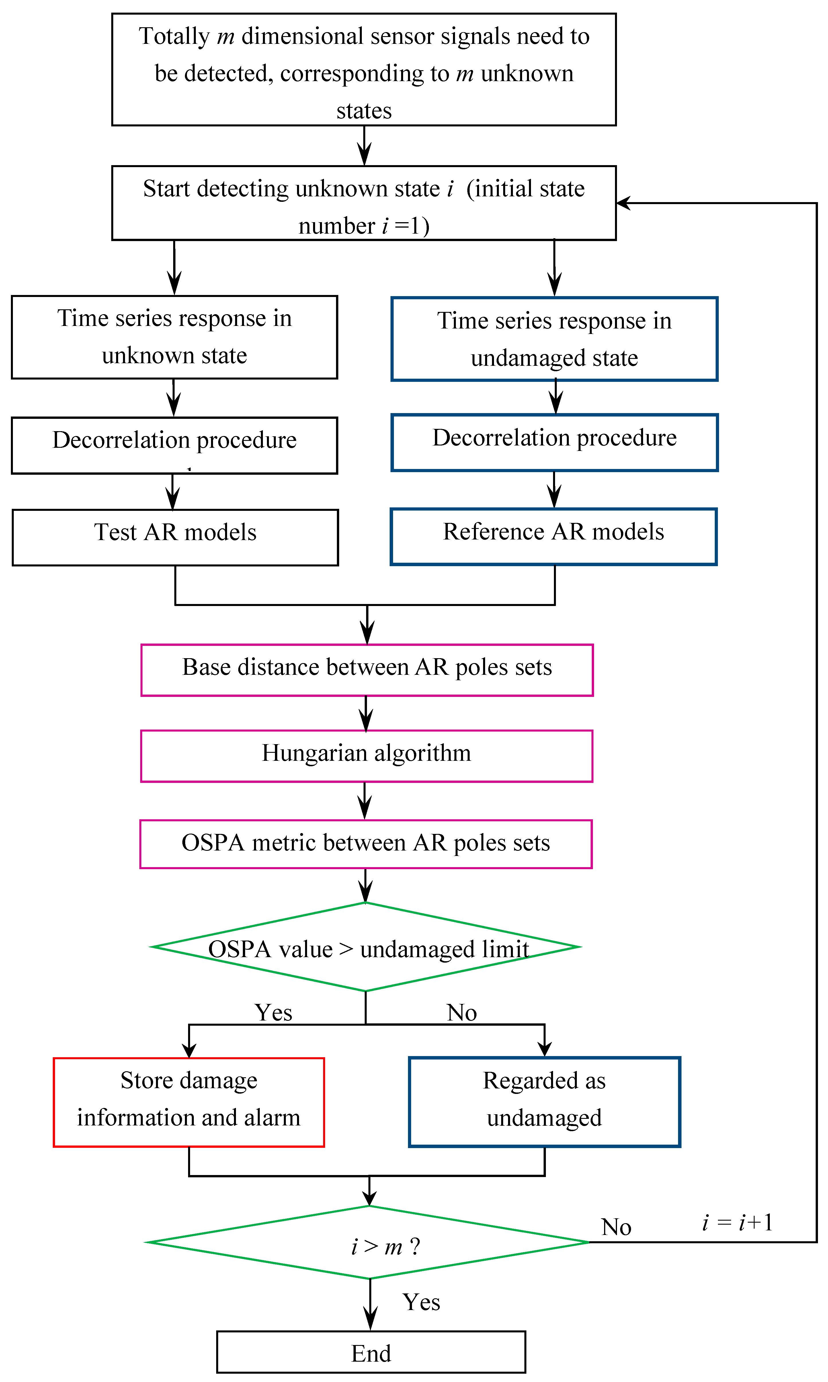
Figure 2.
Flowchart of the proposed damage detection methodology.
Figure 2.
Flowchart of the proposed damage detection methodology.
Figure 3.
Five-story shear building model subjected to: (a) mutually correlated inputs of white noises; (b) earthquake excitation.
Figure 3.
Five-story shear building model subjected to: (a) mutually correlated inputs of white noises; (b) earthquake excitation.
Figure 4.
Time histories of simulated acceleration excited by mutually correlated white noises.
Figure 4.
Time histories of simulated acceleration excited by mutually correlated white noises.
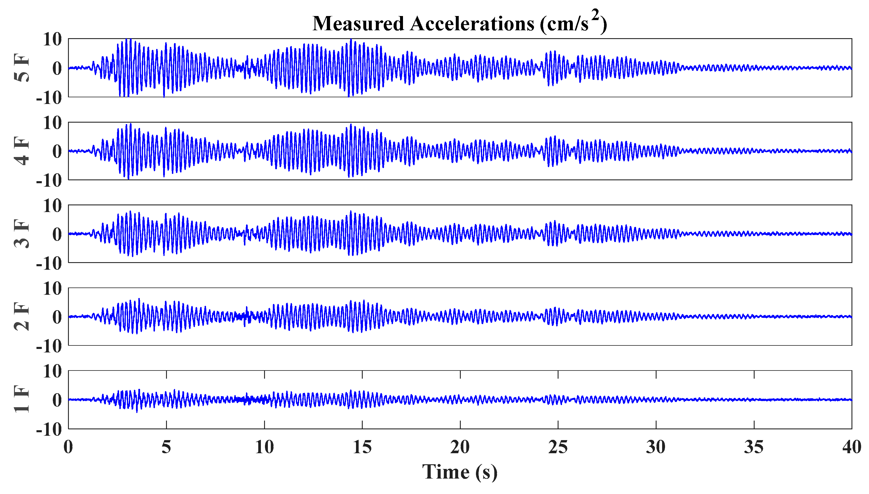
Figure 5.
Time histories of simulated acceleration excited by El Centro earthquake record.
Figure 5.
Time histories of simulated acceleration excited by El Centro earthquake record.
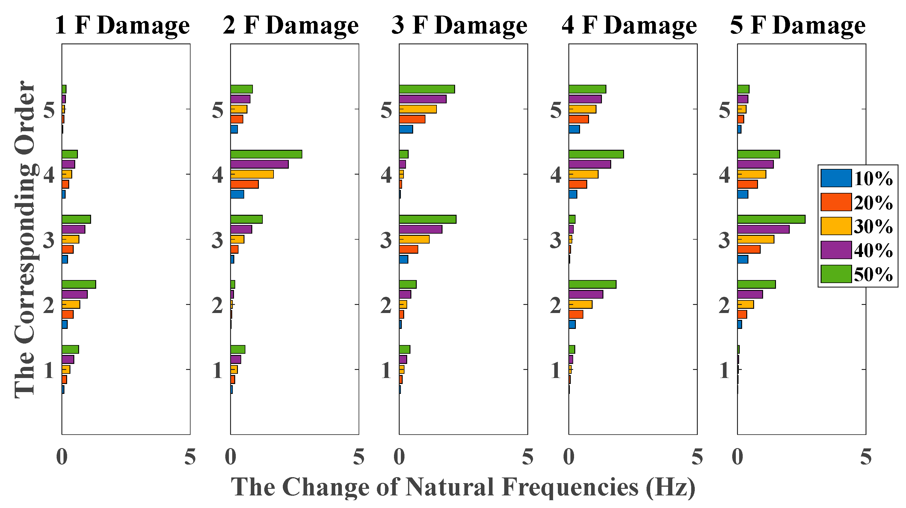
Figure 6.
Damage detection results based on the change of natural frequencies (mutually correlated white noises inputs, 5% noise, data length = 4000).
Figure 6.
Damage detection results based on the change of natural frequencies (mutually correlated white noises inputs, 5% noise, data length = 4000).
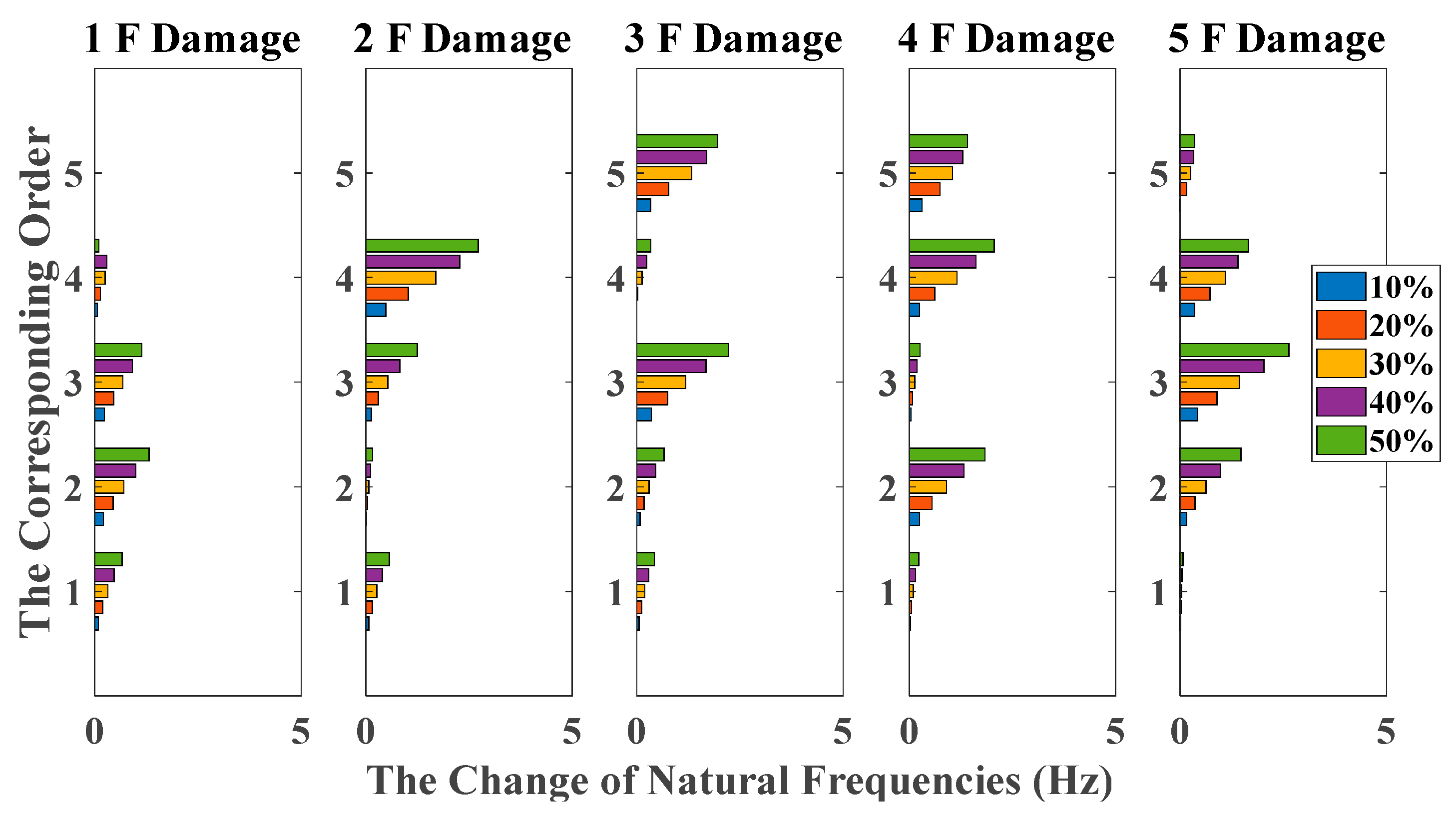
Figure 7.
Damage detection results based on the change of natural frequencies (El Centro earthquake excitation, 5% noise, data length = 4000).
Figure 7.
Damage detection results based on the change of natural frequencies (El Centro earthquake excitation, 5% noise, data length = 4000).
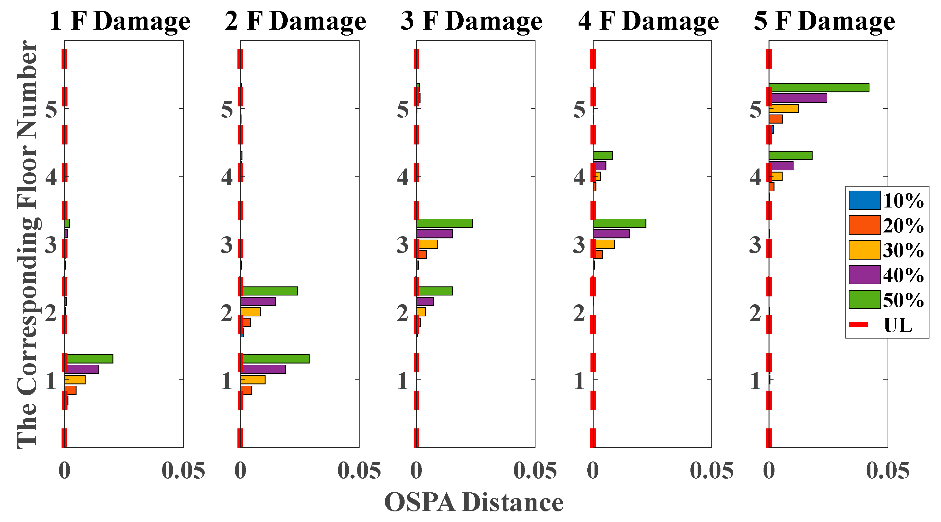
Figure 8.
Damage detection results based on the OSPA distance (mutually correlated white noises inputs, 5% noise, autoregressive model, data length = 4000, AR order = 1, OSPA.p = 2).
Figure 8.
Damage detection results based on the OSPA distance (mutually correlated white noises inputs, 5% noise, autoregressive model, data length = 4000, AR order = 1, OSPA.p = 2).
Figure 9.
Damage detection results based on the OSPA distance (El Centro earthquake excitation, 5% noise, autoregressive model, data length = 4000, AR order = 1, OSPA.p = 2).
Figure 9.
Damage detection results based on the OSPA distance (El Centro earthquake excitation, 5% noise, autoregressive model, data length = 4000, AR order = 1, OSPA.p = 2).
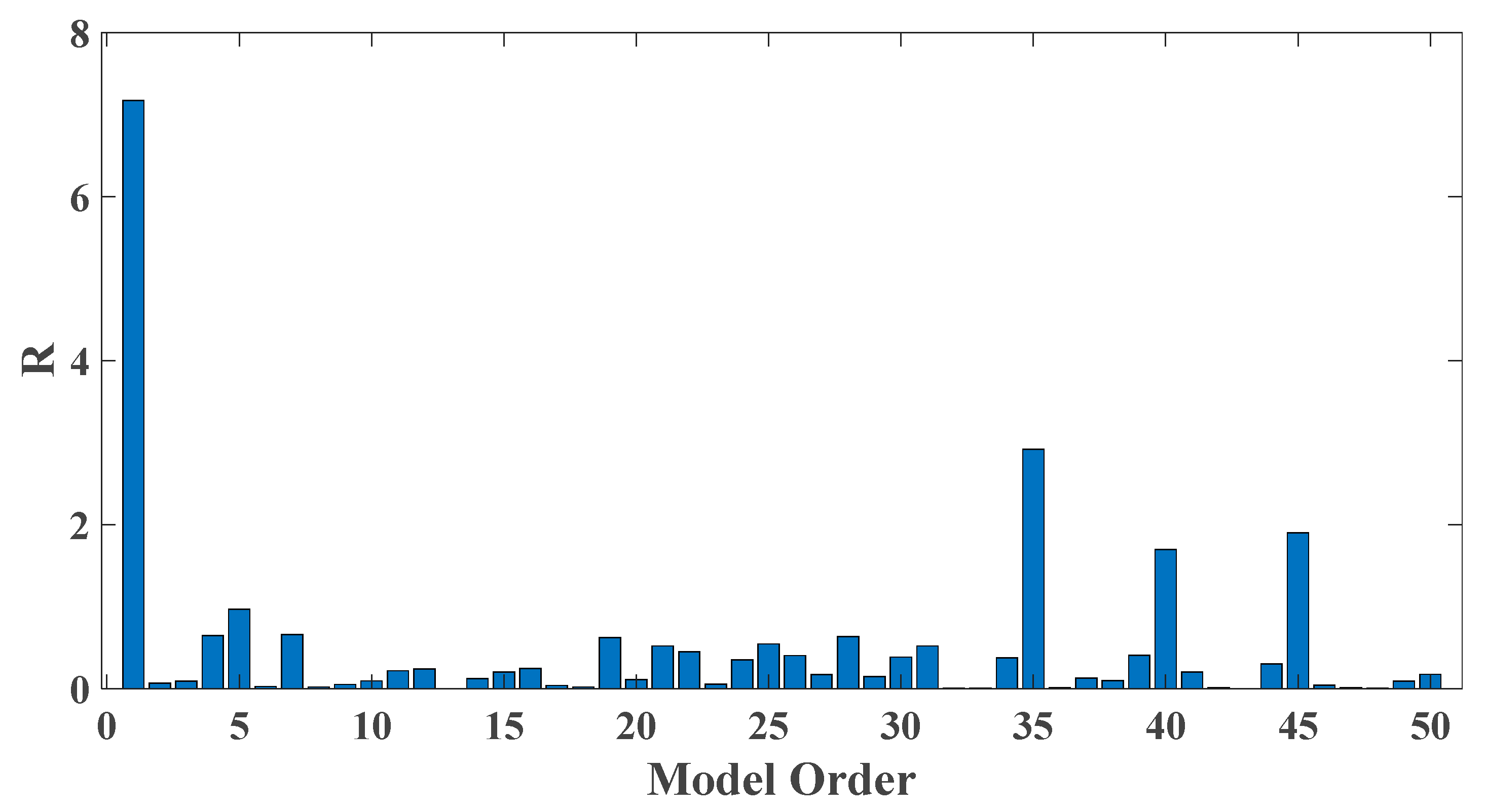
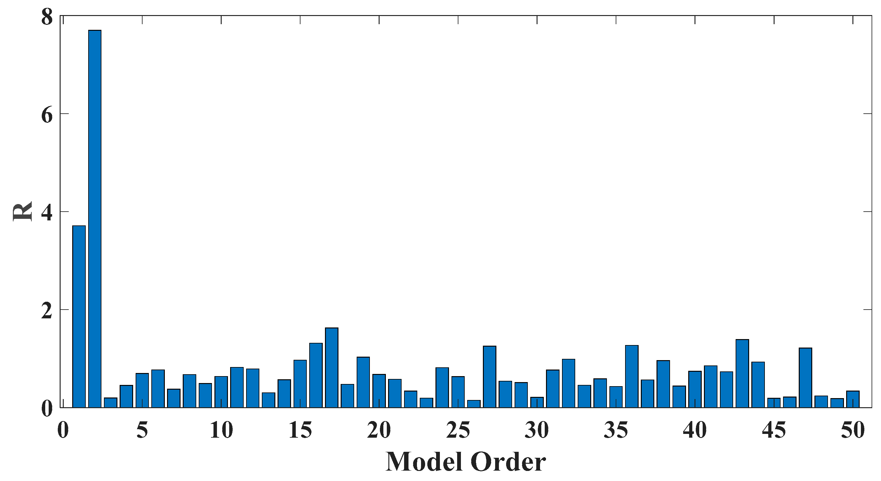
Figure 10.
Evaluation index of damage detection results using various AR orders under the case of 30% damage occurring on the third floor (mutually correlated white noises inputs, 5% noise).
Figure 10.
Evaluation index of damage detection results using various AR orders under the case of 30% damage occurring on the third floor (mutually correlated white noises inputs, 5% noise).
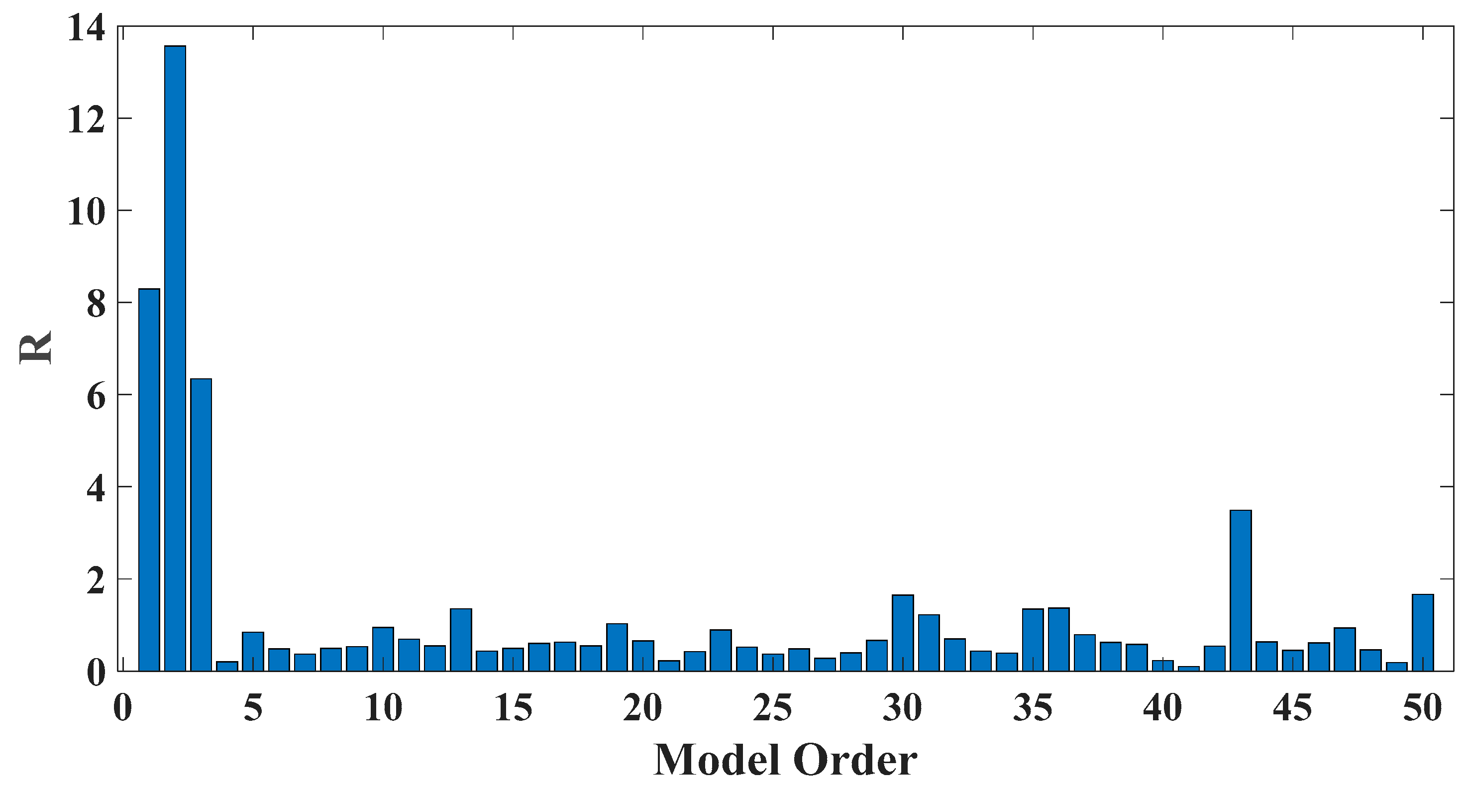
Figure 11.
Evaluation index of damage detection results using various AR orders under the case of 30% damage occurring on the third floor (El Centro earthquake excitation, 5% noise).
Figure 11.
Evaluation index of damage detection results using various AR orders under the case of 30% damage occurring on the third floor (El Centro earthquake excitation, 5% noise).
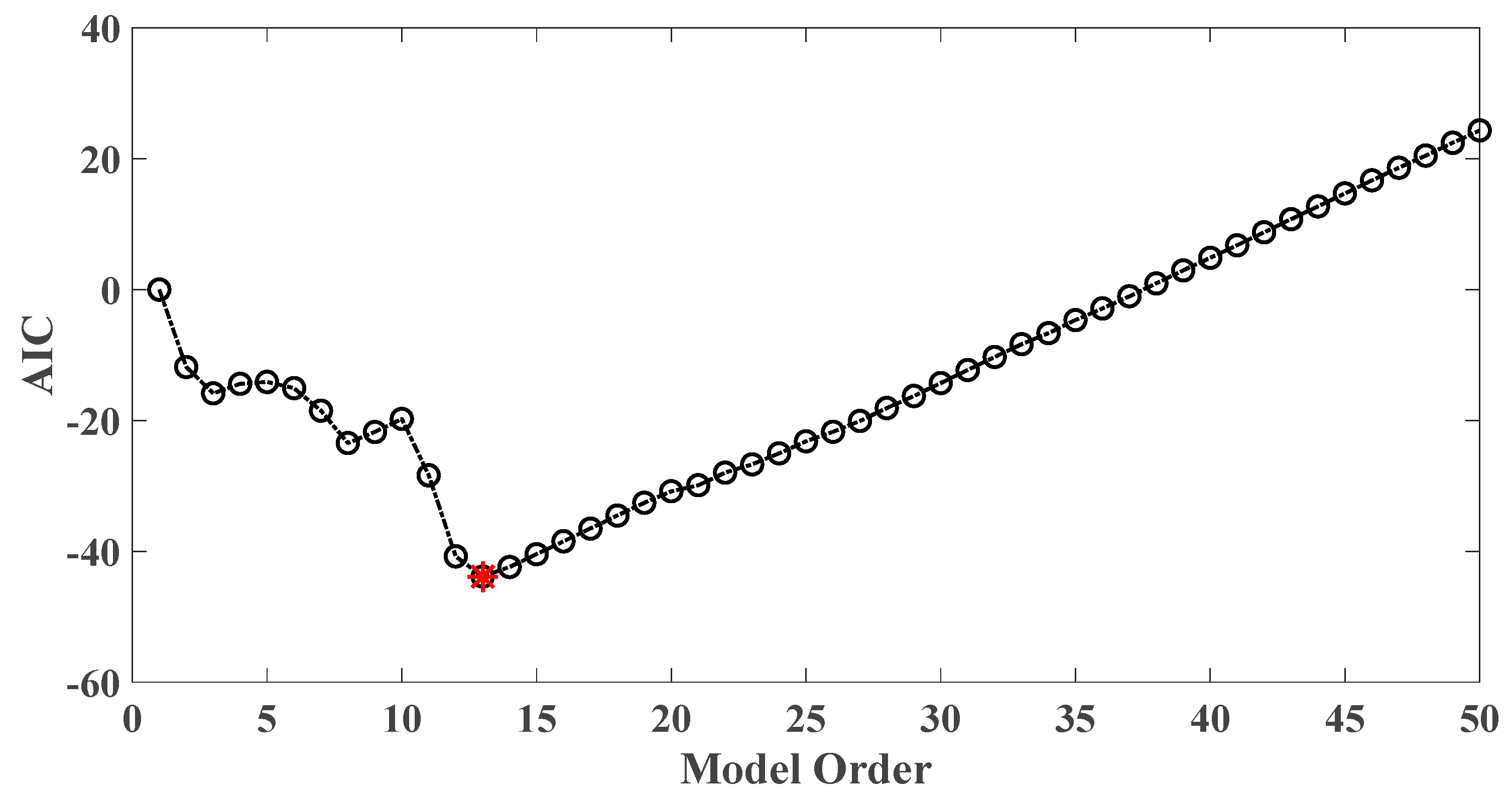
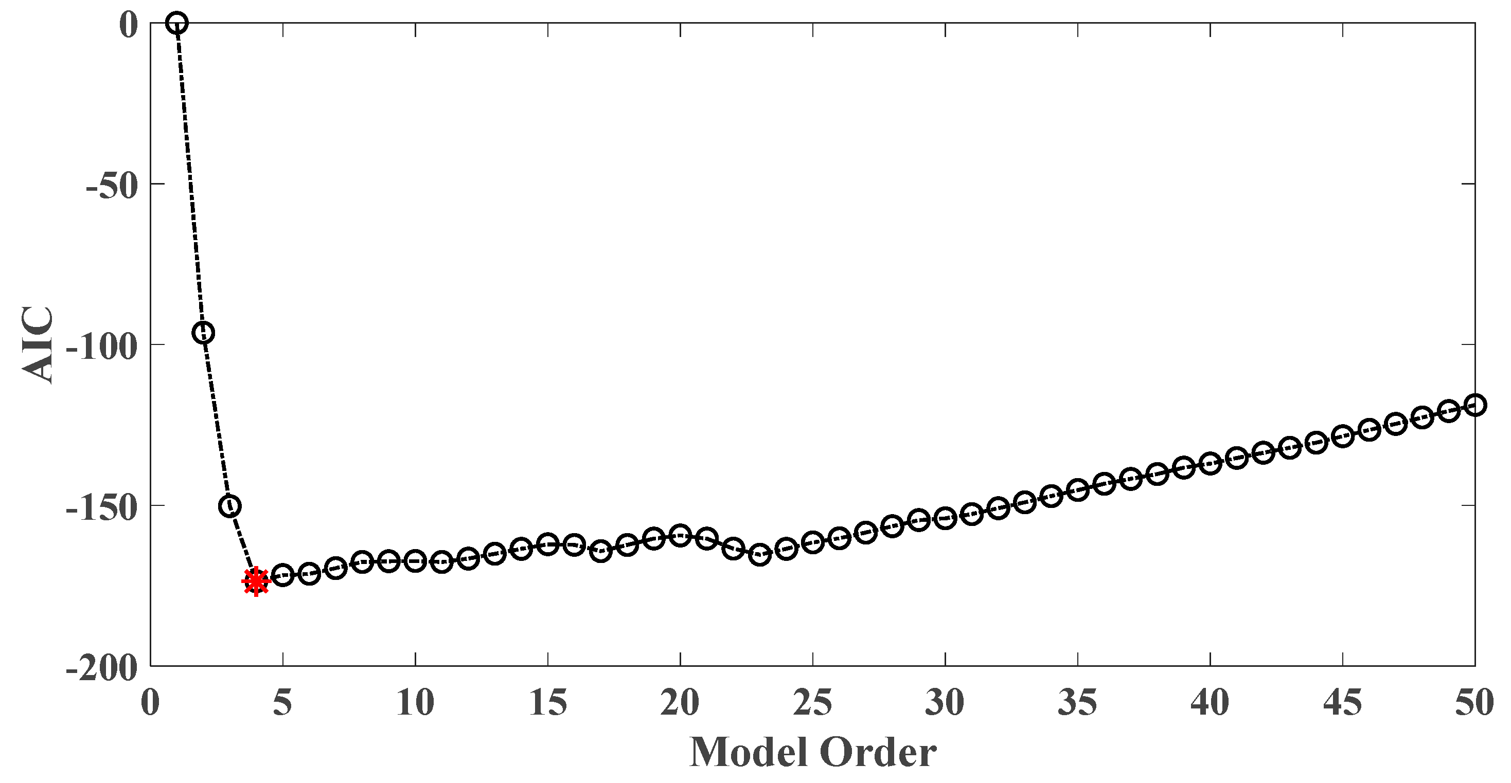
Figure 12.
AIC of an AR model for the third floor response under the case of 30% damage occurring on the third floor (mutually correlated white noises inputs, 5% noise).
Figure 12.
AIC of an AR model for the third floor response under the case of 30% damage occurring on the third floor (mutually correlated white noises inputs, 5% noise).
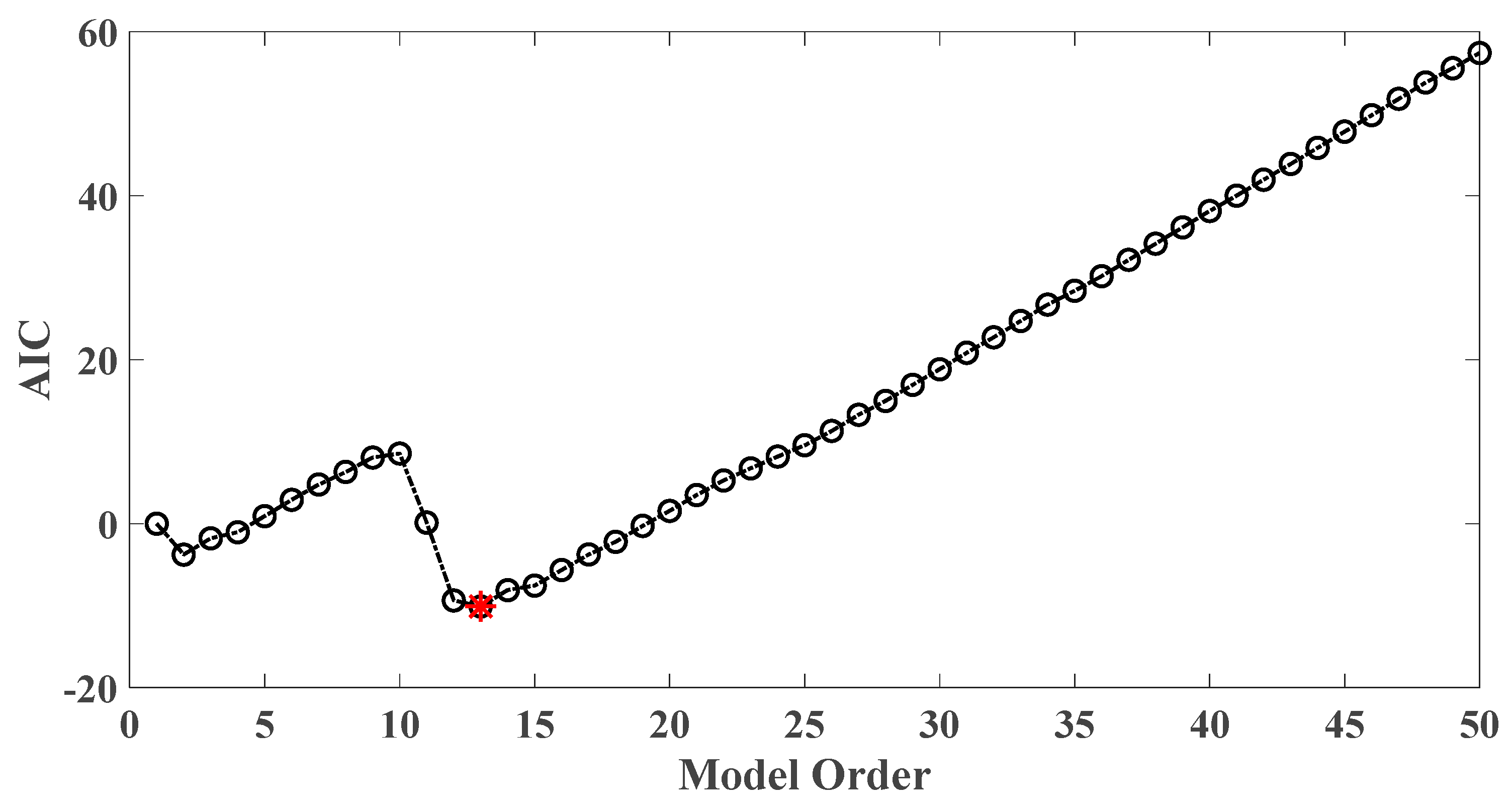
Figure 13.
AIC of an AR model for the third floor response under the case of 30% damage occurring on the third floor (El Centro earthquake excitation, 5% noise).
Figure 13.
AIC of an AR model for the third floor response under the case of 30% damage occurring on the third floor (El Centro earthquake excitation, 5% noise).
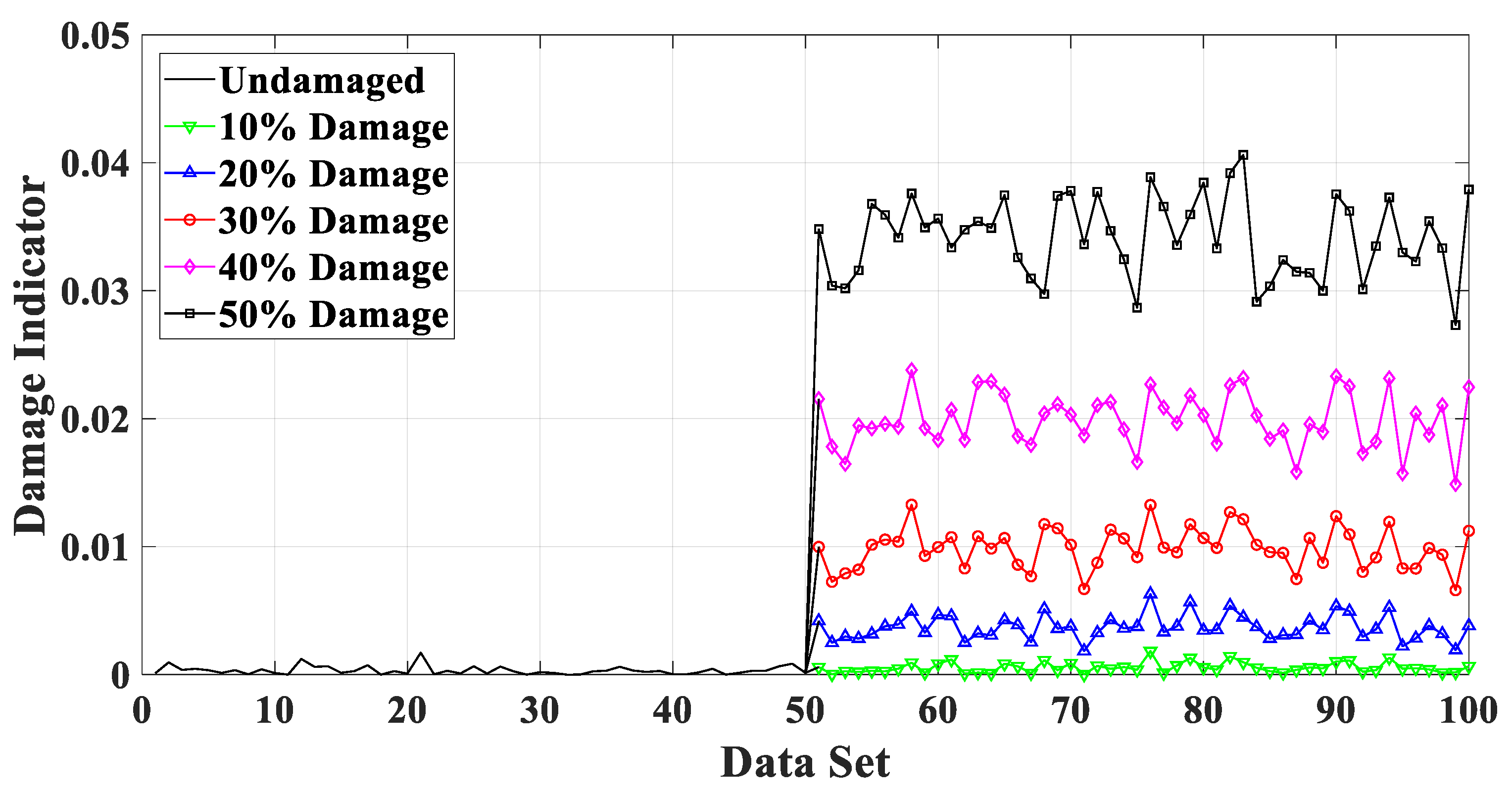
Figure 14.
Damage detection for sudden structural change.
Figure 14.
Damage detection for sudden structural change.
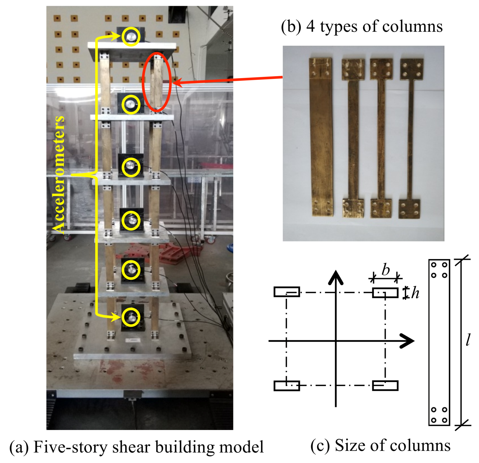
Figure 15.
Experimental setup of five-story shear framework model. (a) Five-story shear building model (b) 4 types of columns. (c) Size of columns.
Figure 15.
Experimental setup of five-story shear framework model. (a) Five-story shear building model (b) 4 types of columns. (c) Size of columns.
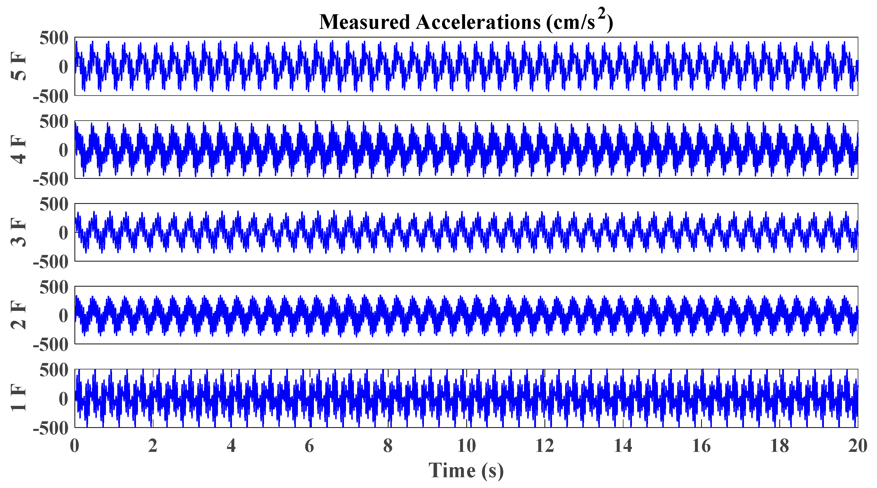
Figure 16.
Typical acceleration time histories of small-scale shear framework structure excited by sine sweeping-frequency excitation.
Figure 16.
Typical acceleration time histories of small-scale shear framework structure excited by sine sweeping-frequency excitation.
Figure 17.
Damage detection results based on the change of natural frequencies (sine sweeping-frequency excitation, data length = 4000).
Figure 17.
Damage detection results based on the change of natural frequencies (sine sweeping-frequency excitation, data length = 4000).
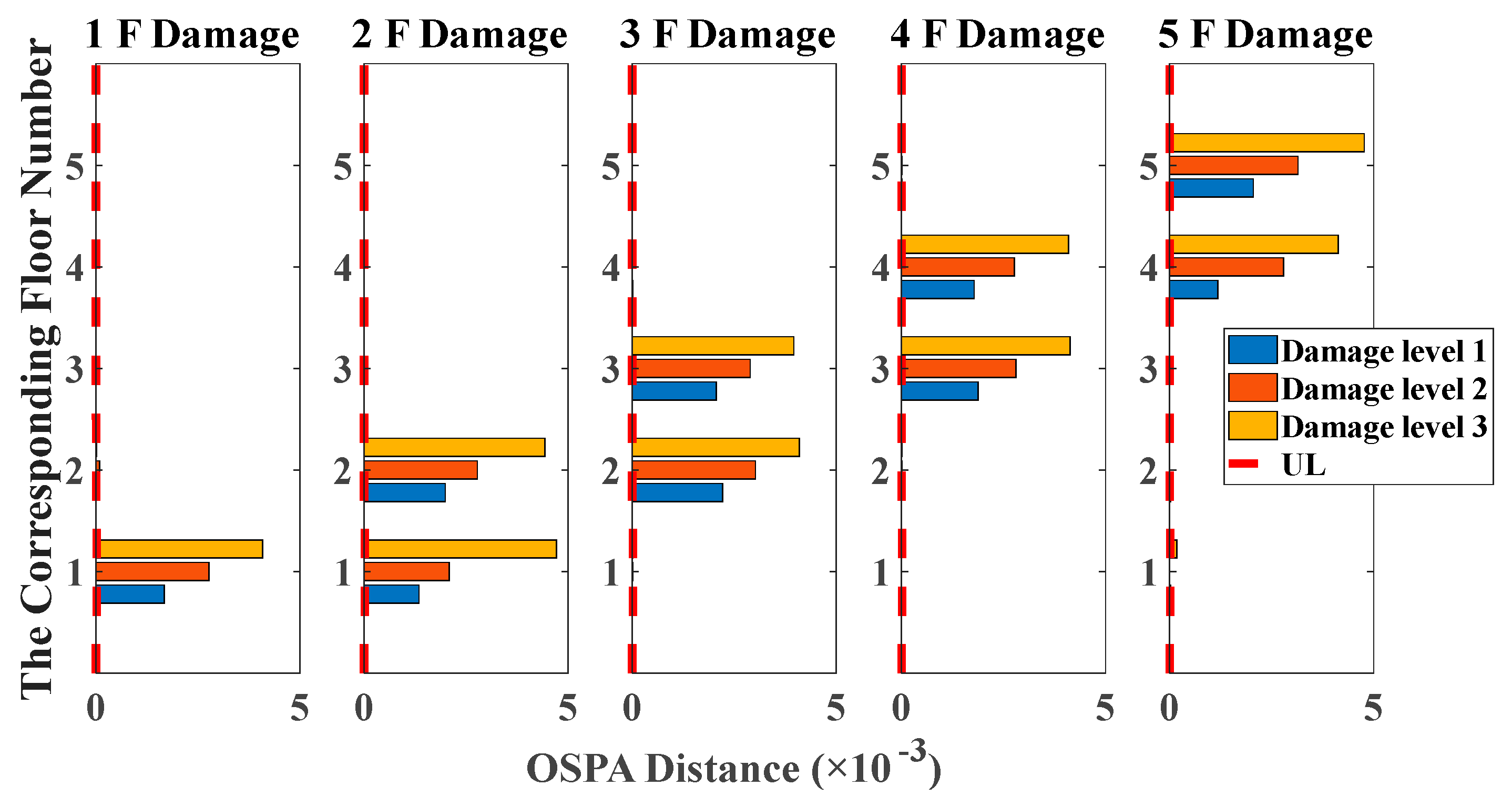
Figure 18.
Damage detection results based on the OSPA distance (sine sweeping-frequency excitation, autoregressive model, data length = 4000, AR order = 1, OSPA.p = 2, Assignment = 1).
Figure 18.
Damage detection results based on the OSPA distance (sine sweeping-frequency excitation, autoregressive model, data length = 4000, AR order = 1, OSPA.p = 2, Assignment = 1).
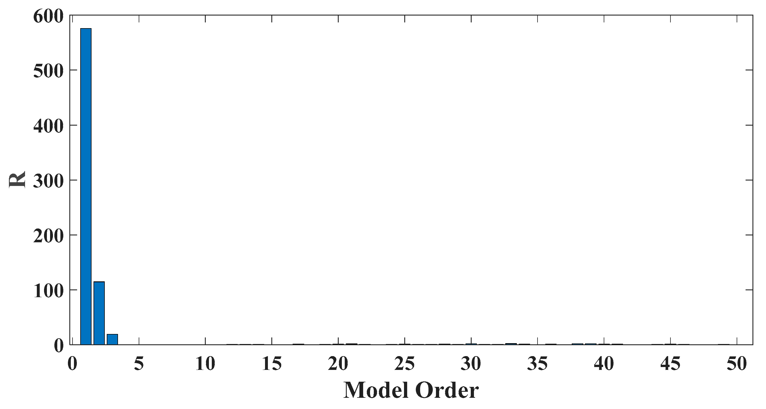
Figure 19.
AIC of an AR model for the third floor response under the case of level 2 damage occurring on the third floor.
Figure 19.
AIC of an AR model for the third floor response under the case of level 2 damage occurring on the third floor.
Figure 20.
Evaluation index of damage detection results using various AR orders (the case of level 2 damage occurring on the third floor).
Figure 20.
Evaluation index of damage detection results using various AR orders (the case of level 2 damage occurring on the third floor).
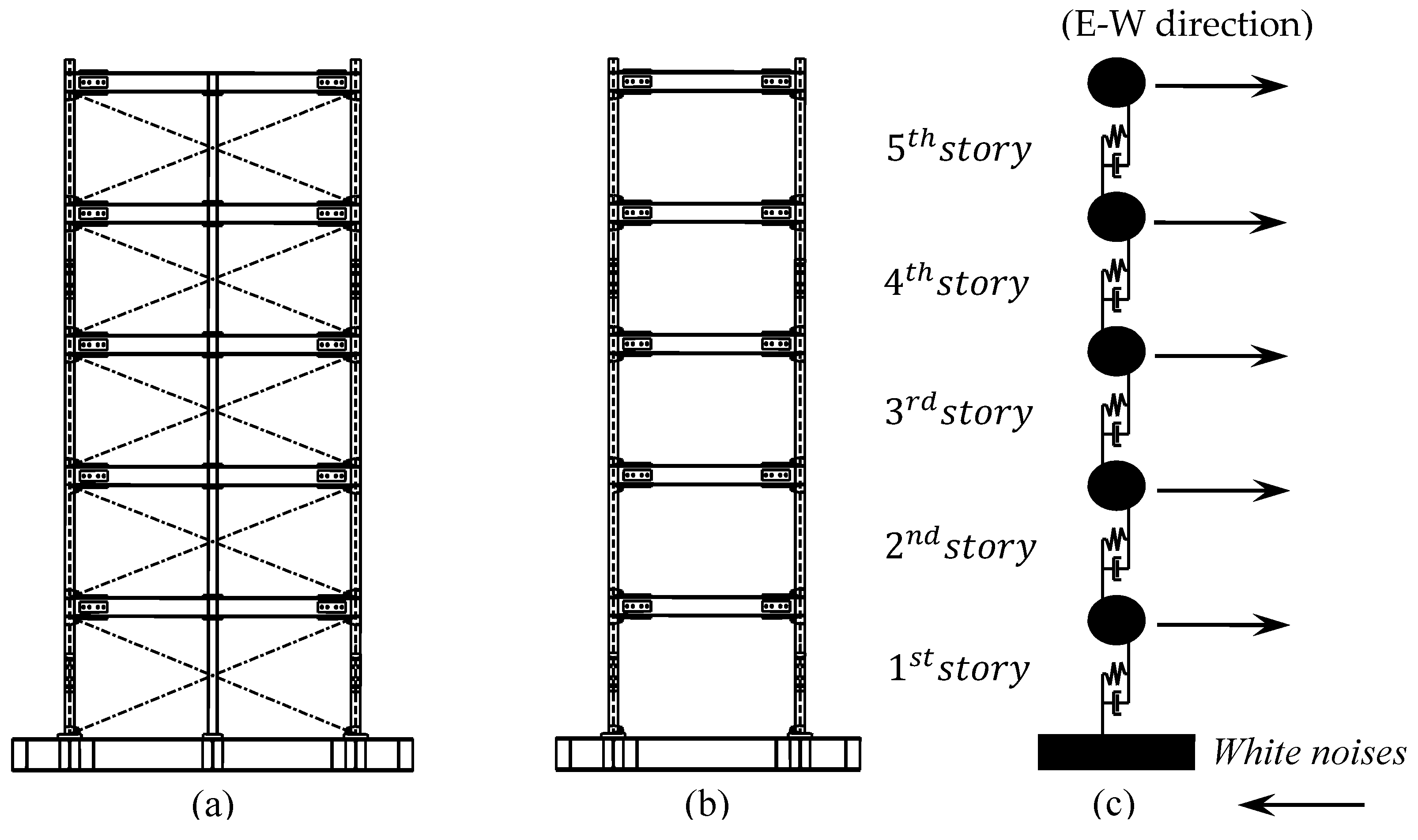
Figure 21.
Experimental building model: (a) E-W direction; (b) N-S direction; (c) Simplified shear building model.
Figure 21.
Experimental building model: (a) E-W direction; (b) N-S direction; (c) Simplified shear building model.
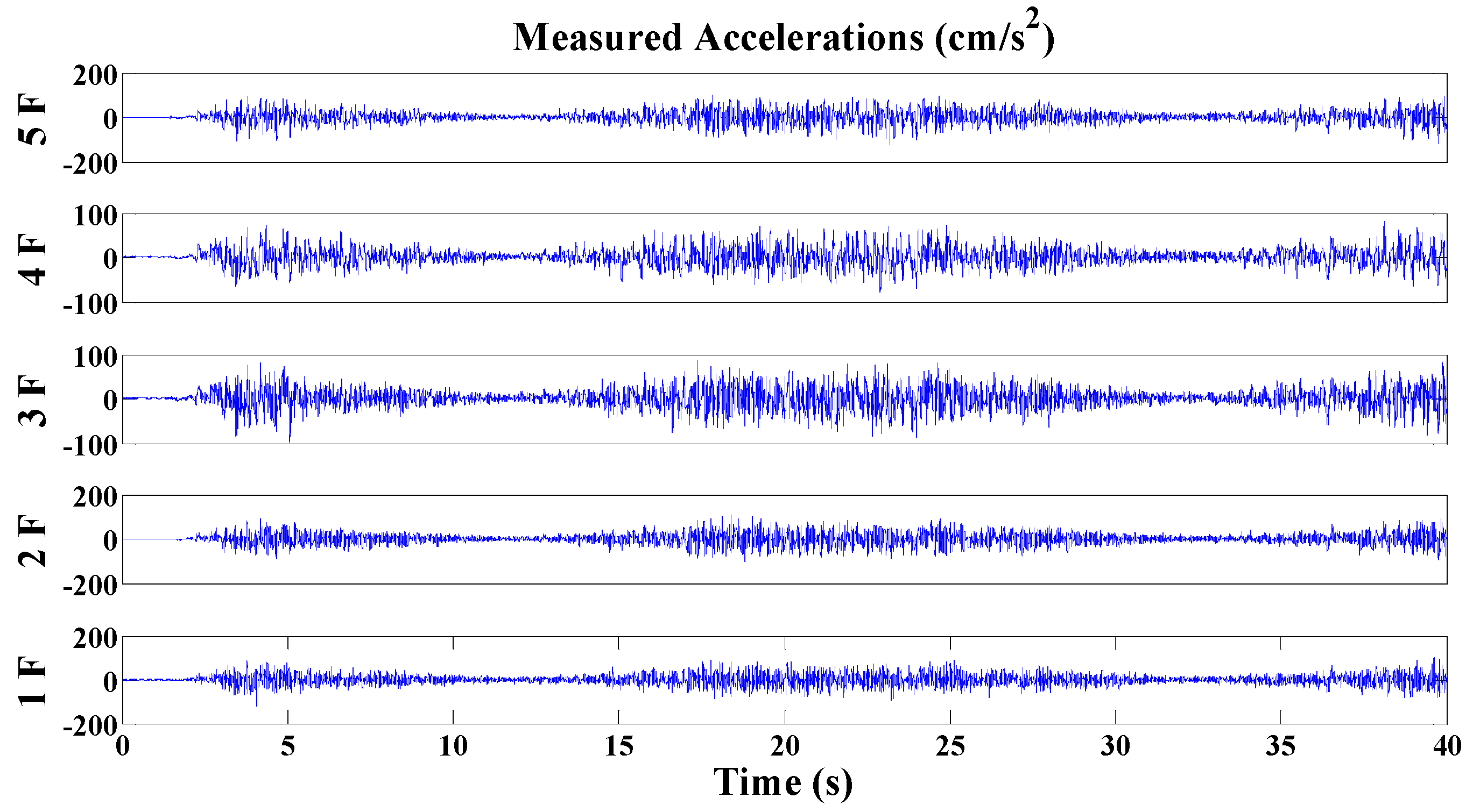
Figure 22.
Acceleration time histories of the large-scale framework model excited by a shaking table.
Figure 22.
Acceleration time histories of the large-scale framework model excited by a shaking table.
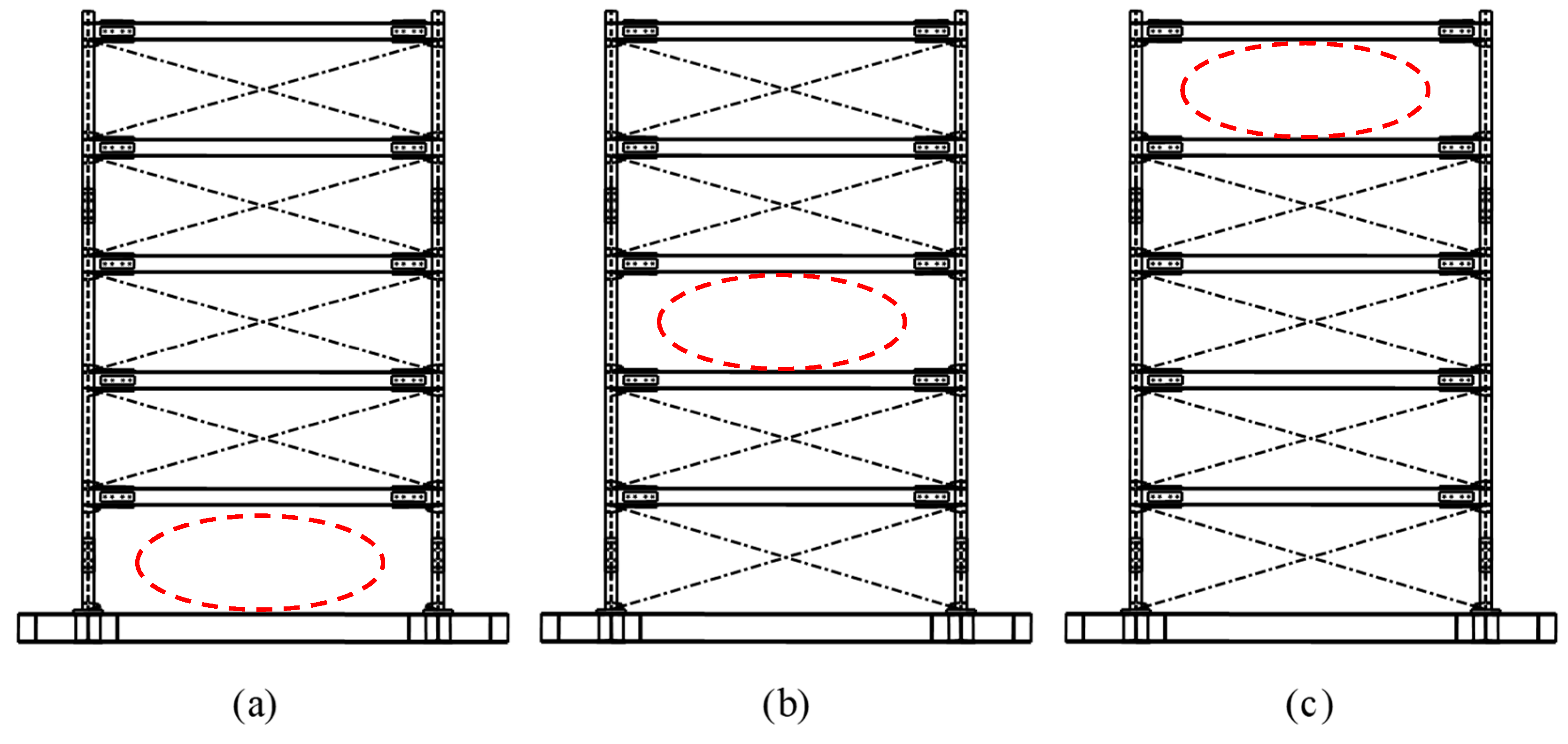
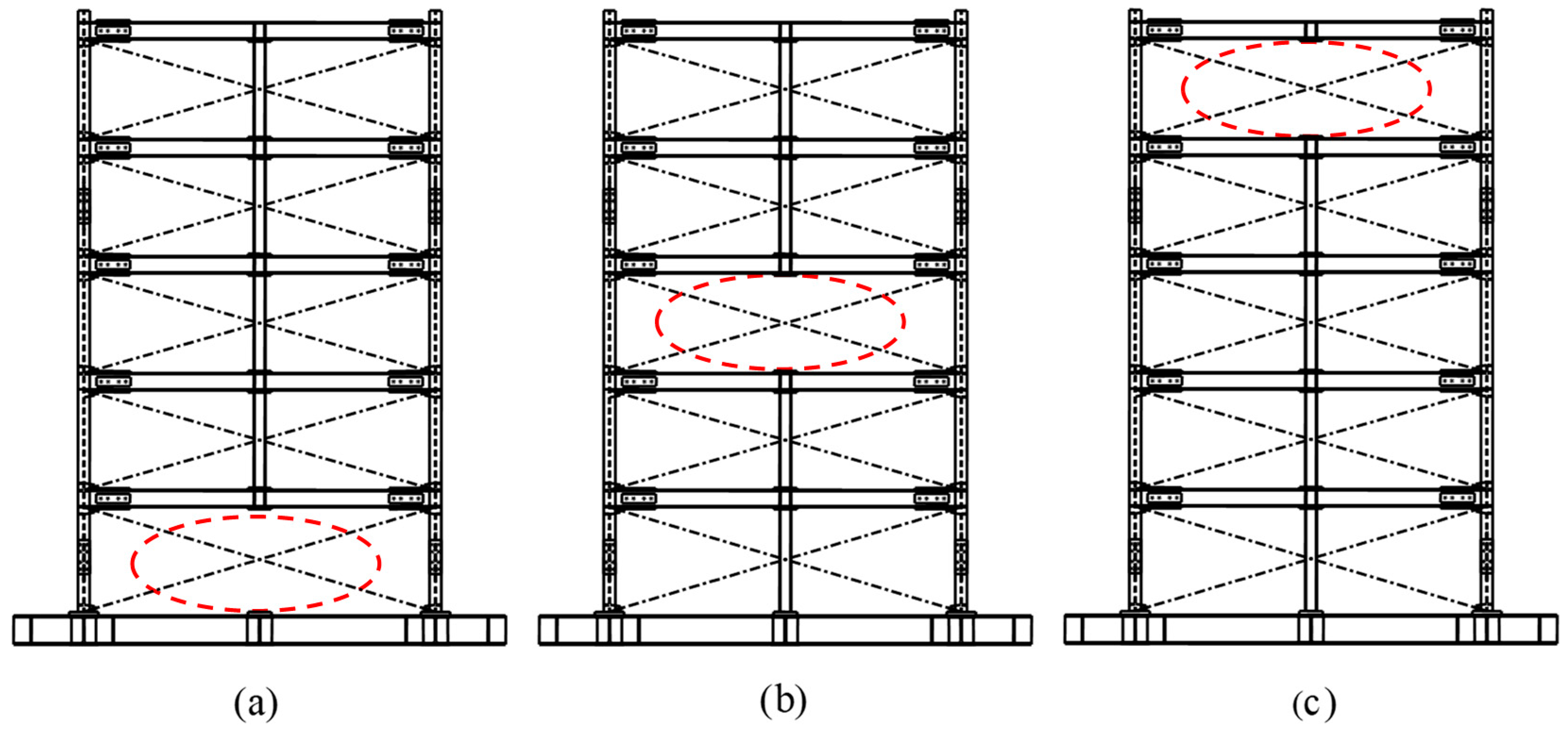
Figure 23.
Damage cases: removing braces on the (a) first; (b) third; and (c) fifth story.
Figure 23.
Damage cases: removing braces on the (a) first; (b) third; and (c) fifth story.
Figure 24.
Damage cases: removing central column on the (a) first; (b) third; and (c) fifth story.
Figure 24.
Damage cases: removing central column on the (a) first; (b) third; and (c) fifth story.
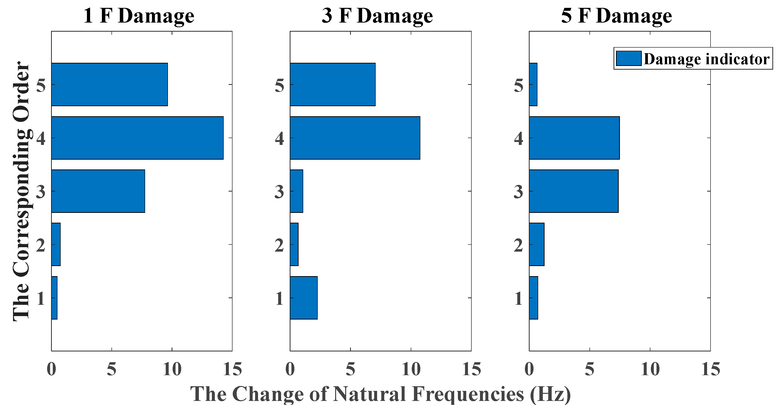
Figure 25.
Damage detection results based on the change of natural frequencies (removing braces, white noises excitation, data length = 4000).
Figure 25.
Damage detection results based on the change of natural frequencies (removing braces, white noises excitation, data length = 4000).
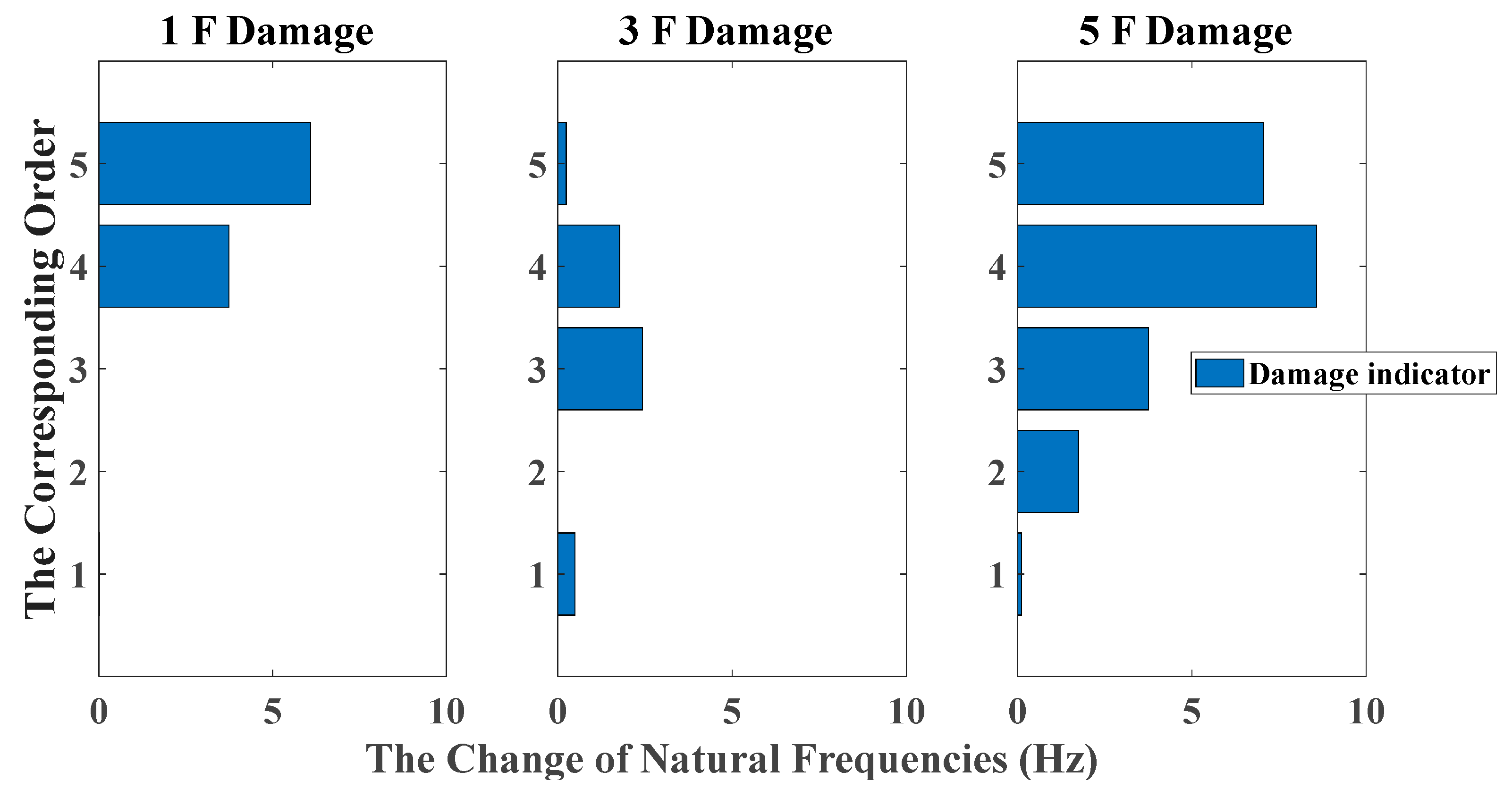
Figure 26.
Damage detection results based on the change of natural frequencies (removing central columns, white noises excitation, data length = 4000).
Figure 26.
Damage detection results based on the change of natural frequencies (removing central columns, white noises excitation, data length = 4000).
Figure 27.
Damage detection results based on the OSPA distance (removing braces, white noises excitation, autoregressive model, data length = 4000, AR order = 2, OSPA.p = 2).
Figure 27.
Damage detection results based on the OSPA distance (removing braces, white noises excitation, autoregressive model, data length = 4000, AR order = 2, OSPA.p = 2).
Figure 28.
Damage detection results based on the OSPA distance (removing central columns, white noises excitation, autoregressive model, data length = 4000, AR order = 2, OSPA.p = 2).
Figure 28.
Damage detection results based on the OSPA distance (removing central columns, white noises excitation, autoregressive model, data length = 4000, AR order = 2, OSPA.p = 2).
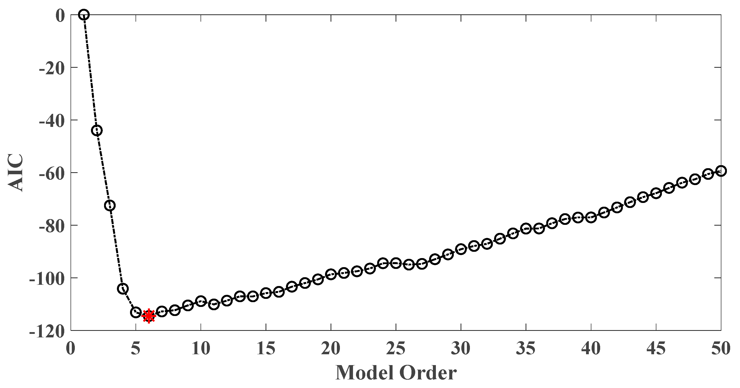
Figure 29.
AIC of an AR model for the third floor response under the case of removing braces on the third floor.
Figure 29.
AIC of an AR model for the third floor response under the case of removing braces on the third floor.
Figure 30.
AIC of an AR model for the third floor response under the case of removing central columns on the third floor.
Figure 30.
AIC of an AR model for the third floor response under the case of removing central columns on the third floor.
Figure 31.
Evaluation index of damage detection results using various AR orders (the case of removing braces on the third floor).
Figure 31.
Evaluation index of damage detection results using various AR orders (the case of removing braces on the third floor).
Figure 32.
Evaluation index of damage detection results using various AR orders (the case of removing central columns on the third floor).
Figure 32.
Evaluation index of damage detection results using various AR orders (the case of removing central columns on the third floor).
Table 1.
OSPA distance and the corresponding parameters for the case of damage occurring on the first floor (mutually correlated white noises inputs, 5% noise, autoregressive model, data length = 4000, AR order = 1, OSPA.p = 2, Assignment = 1).
Table 1.
OSPA distance and the corresponding parameters for the case of damage occurring on the first floor (mutually correlated white noises inputs, 5% noise, autoregressive model, data length = 4000, AR order = 1, OSPA.p = 2, Assignment = 1).
| Damage (%) | Floor | Pole | D | OSPA Distance |
|---|
| 10 | 1 | 0.0845 | 1.4323 × 10⁻³ | 0.0014 |
| 0 | 2 | 0.2531 | 1.7889 × 10⁻⁴ | 0.0002 |
| 0 | 3 | 0.2286 | 5.3499 × 10⁻⁴ | 0.0005 |
| 0 | 4 | 0.2405 | 7.6139 × 10⁻⁵ | 0.0001 |
| 0 | 5 | 0.5691 | 1.3142 × 10⁻⁴ | 0.0001 |
| 20 | 1 | 0.1167 | 4.9122 × 10⁻³ | 0.0049 |
| 0 | 2 | 0.2563 | 2.7335 × 10⁻⁴ | 0.0003 |
| 0 | 3 | 0.2219 | 2.6851 × 10⁻⁴ | 0.0003 |
| 0 | 4 | 0.2350 | 1.0079 × 10⁻⁵ | 0.0000 |
| 0 | 5 | 0.5675 | 9.7644 × 10⁻⁵ | 0.0001 |
| 30 | 1 | 0.1403 | 8.7681 × 10⁻³ | 0.0088 |
| 0 | 2 | 0.2620 | 4.9483 × 10⁻⁴ | 0.0005 |
| 0 | 3 | 0.2255 | 4.0167 × 10⁻⁴ | 0.0004 |
| 0 | 4 | 0.2311 | 5.4253 × 10⁻⁷ | 0.0000 |
| 0 | 5 | 0.5563 | 1.7813 × 10⁻⁶ | 0.0000 |
| 40 | 1 | 0.1668 | 1.4434 × 10⁻² | 0.0144 |
| 0 | 2 | 0.2684 | 8.2036 × 10⁻⁴ | 0.0008 |
| 0 | 3 | 0.2397 | 1.1705 × 10⁻³ | 0.0012 |
| 0 | 4 | 0.2344 | 6.7463 × 10⁻⁶ | 0.0000 |
| 0 | 5 | 0.5527 | 2.4542 × 10⁻⁵ | 0.0000 |
| 50 | 1 | 0.1894 | 2.0398 × 10⁻² | 0.0204 |
| 0 | 2 | 0.2707 | 9.5958 × 10⁻⁴ | 0.0010 |
| 0 | 3 | 0.2500 | 1.9784 × 10⁻³ | 0.0020 |
| 0 | 4 | 0.2409 | 8.2837 × 10⁻⁵ | 0.0001 |
| 0 | 5 | 0.5510 | 4.4383 × 10⁻⁵ | 0.0000 |
Table 2.
OSPA distance and the corresponding parameters for the case of damage occurring on the first floor (El Centro earthquake excitation, 5% noise, autoregressive model, data length = 4000, AR order = 1, OSPA.p = 2, Assignment = 1).
Table 2.
OSPA distance and the corresponding parameters for the case of damage occurring on the first floor (El Centro earthquake excitation, 5% noise, autoregressive model, data length = 4000, AR order = 1, OSPA.p = 2, Assignment = 1).
| Damage (%) | Floor | Pole | D | OSPA Distance |
|---|
| 10 | 1 | 0.2554 | 5.3738 × 10⁻⁴ | 0.0005 |
| 0 | 2 | 0.3177 | 4.8151 × 10⁻⁵ | 0.0000 |
| 0 | 3 | 0.3236 | 2.1281 × 10⁻⁷ | 0.0000 |
| 0 | 4 | 0.3339 | 4.5140 × 10⁻⁵ | 0.0000 |
| 0 | 5 | 0.5858 | 1.0910 × 10⁻⁵ | 0.0000 |
| 20 | 1 | 0.2676 | 1.2545 × 10⁻³ | 0.0013 |
| 0 | 2 | 0.3277 | 2.8711 × 10⁻⁴ | 0.0003 |
| 0 | 3 | 0.3179 | 3.8201 × 10⁻⁵ | 0.0000 |
| 0 | 4 | 0.3393 | 1.4790 × 10⁻⁴ | 0.0001 |
| 0 | 5 | 0.5793 | 9.5872 × 10⁻⁵ | 0.0001 |
| 30 | 1 | 0.2915 | 3.5150 × 10⁻³ | 0.0035 |
| 0 | 2 | 0.3269 | 2.6204 × 10⁻⁴ | 0.0003 |
| 0 | 3 | 0.3161 | 6.3640 × 10⁻⁵ | 0.0001 |
| 0 | 4 | 0.3361 | 7.9809 × 10⁻⁵ | 0.0001 |
| 0 | 5 | 0.5799 | 8.4547 × 10⁻⁵ | 0.0001 |
| 40 | 1 | 0.3138 | 6.6601 × 10⁻³ | 0.0067 |
| 0 | 2 | 0.3248 | 1.9730 × 10⁻⁴ | 0.0002 |
| 0 | 3 | 0.3114 | 1.6101 × 10⁻⁴ | 0.0002 |
| 0 | 4 | 0.3395 | 1.5355 × 10⁻⁴ | 0.0002 |
| 0 | 5 | 0.5748 | 2.0421 × 10⁻⁴ | 0.0002 |
| 50 | 1 | 0.3302 | 9.5953 × 10⁻³ | 0.0096 |
| 0 | 2 | 0.3243 | 1.8263 × 10⁻⁴ | 0.0002 |
| 0 | 3 | 0.2909 | 1.0986 × 10⁻³ | 0.0011 |
| 0 | 4 | 0.3411 | 1.9605 × 10⁻⁴ | 0.0002 |
| 0 | 5 | 0.5530 | 1.3033 × 10⁻³ | 0.0013 |
Table 3.
Specific physical parameters of the columns.
Table 3.
Specific physical parameters of the columns.
| Column | Section h × b × l (m3) | Theoretical Lateral Stiffness (N/m) | State |
|---|
| Type 0 | 0.003 × 0.030 × 0.24 | 1.1809 × 10⁴ | Undamaged |
| Type 1 | 0.003 × 0.014 × 0.24 | 5.5110 × 10³ | 53.33% Damage |
| Type 2 | 0.003 × 0.010 × 0.24 | 3.9364 × 10³ | 66.67% Damage |
| Type 3 | 0.003 × 0.006 × 0.24 | 2.3619 × 10³ | 80.00% Damage |
Table 4.
OSPA distance and the corresponding parameters for the case of damage occurring on the first floor (sine sweeping-frequency excitation, autoregressive model, data length = 4000, AR order = 1, OSPA.p = 2, Assignment = 1).
Table 4.
OSPA distance and the corresponding parameters for the case of damage occurring on the first floor (sine sweeping-frequency excitation, autoregressive model, data length = 4000, AR order = 1, OSPA.p = 2, Assignment = 1).
| Damage (%) | Floor | Pole | D | OSPA Distance |
|---|
| 53.33 | 1 | 0.8875 | 1.6746 × 10⁻³ | 0.0017 |
| 0 | 2 | 0.8405 | 6.6544 × 10⁻⁶ | 0.0000 |
| 0 | 3 | 0.8374 | 1.8927 × 10⁻⁶ | 0.0000 |
| 0 | 4 | 0.8325 | 9.7249 × 10⁻⁶ | 0.0000 |
| 0 | 5 | 0.9097 | 8.4550 × 10⁻⁶ | 0.0000 |
| 66.67 | 1 | 0.8992 | 2.7698 × 10⁻³ | 0.0028 |
| 0 | 2 | 0.8478 | 9.6323 × 10⁻⁵ | 0.0001 |
| 0 | 3 | 0.8408 | 2.2149 × 10⁻⁵ | 0.0000 |
| 0 | 4 | 0.8368 | 1.3291 × 10⁻⁶ | 0.0000 |
| 0 | 5 | 0.9121 | 2.4982 × 10⁻⁷ | 0.0000 |
| 80.00 | 1 | 0.9105 | 4.0871 × 10⁻³ | 0.0041 |
| 0 | 2 | 0.8422 | 1.8414 × 10⁻⁵ | 0.0000 |
| 0 | 3 | 0.8362 | 9.6462 × 10⁻⁹ | 0.0000 |
| 0 | 4 | 0.8381 | 6.3794 × 10⁻⁶ | 0.0000 |
| 0 | 5 | 0.9161 | 1.2693 × 10⁻⁵ | 0.0000 |
Table 5.
Modal characteristics of the experimental building model.
Table 5.
Modal characteristics of the experimental building model.
| Mode | Natural Frequency (Hz) | Damping Ratio (%) |
|---|
| 1 | 2.93 | 0.17 |
| 2 | 8.91 | 0.14 |
| 3 | 14.82 | 0.13 |
| 4 | 20.33 | 0.08 |
| 5 | 24.40 | 0.05 |
Table 6.
OSPA distance and the corresponding parameters for the case of removing braces on the first floor (white noises excitation, autoregressive model, data length = 4000, AR order = 2, OSPA.p = 2).
Table 6.
OSPA distance and the corresponding parameters for the case of removing braces on the first floor (white noises excitation, autoregressive model, data length = 4000, AR order = 2, OSPA.p = 2).
| Damage | Floor | Pole | D | Assignment | OSPA Distance |
|---|
| Removing | 1 | 0.6667 ± 0.5754i | 0.0408 | 1.6938 | 1 | 0 | 0.0408 |
| braces | | | 1.6938 | 0.0408 | 0 | 1 | |
| 0 | 2 | 0.5520 ± 0.6307i | 0.0065 | 1.7785 | 1 | 0 | 0.0065 |
| | | | 1.7785 | 0.0065 | 0 | 1 | |
| 0 | 3 | 0.5710 ± 0.6322i | 0.0078 | 1.7823 | 1 | 0 | 0.0078 |
| | | | 1.7823 | 0.0078 | 0 | 1 | |
| 0 | 4 | 0.5716 ± 0.6117i | 0.0053 | 1.6293 | 1 | 0 | 0.0053 |
| | | | 1.6293 | 0.0053 | 0 | 1 | |
| 0 | 5 | 0.7160 ± 0.5228i | 0.0033 | 1.1546 | 1 | 0 | 0.0033 |
| | | | 1.1546 | 0.0033 | 0 | 1 | |
Table 7.
OSPA distance and the corresponding parameters for the case of removing columns on the first floor (white noises excitation, autoregressive model, data length = 4000, AR order = 2, OSPA.p = 2).
Table 7.
OSPA distance and the corresponding parameters for the case of removing columns on the first floor (white noises excitation, autoregressive model, data length = 4000, AR order = 2, OSPA.p = 2).
| Damage | Floor | Pole | D | Assignment | OSPA Distance |
|---|
| Removing | 1 | 0.7890 ± 0.5326i | 0.0051 | 1.2227 | 1 | 0 | 0.0051 |
| columns | | | 1.2227 | 0.0051 | 0 | 1 | |
| 0 | 2 | 0.7231 ± 0.5873i | 0.0004 | 1.3890 | 1 | 0 | 0.0004 |
| | | | 1.3890 | 0.0004 | 0 | 1 | |
| 0 | 3 | 0.7202 ± 0.5862i | 0.0002 | 1.3895 | 1 | 0 | 0.0002 |
| | | | 1.3895 | 0.0002 | 0 | 1 | |
| 0 | 4 | 0.7260 ± 0.5780i | 0.0002 | 1.3496 | 1 | 0 | 0.0003 |
| | | | 1.3496 | 0.0002 | 0 | 1 | |
| 0 | 5 | 0.8310 ± 0.4280i | 0.0007 | 0.7145 | 1 | 0 | 0.0007 |
| | | | 0.7145 | 0.0007 | 0 | 1 | |


