Long-Term Performance Assessment of Low-Cost Atmospheric Sensors in the Arctic Environment


 ,
,  , , , , ,
  and
and 
Abstract
1. Introduction
2. Materials and Methods
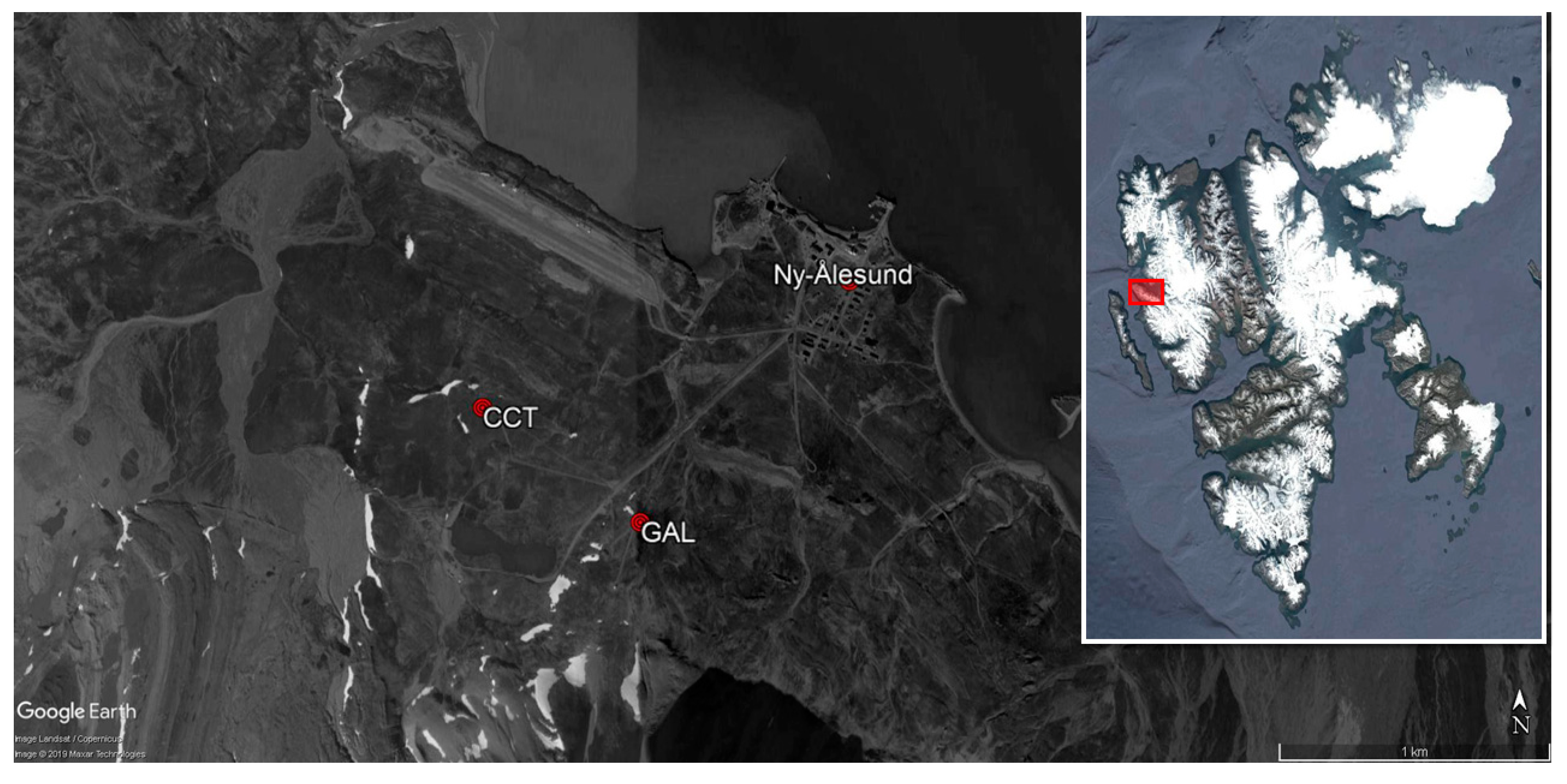
2.1. Study Area and Reference Stations
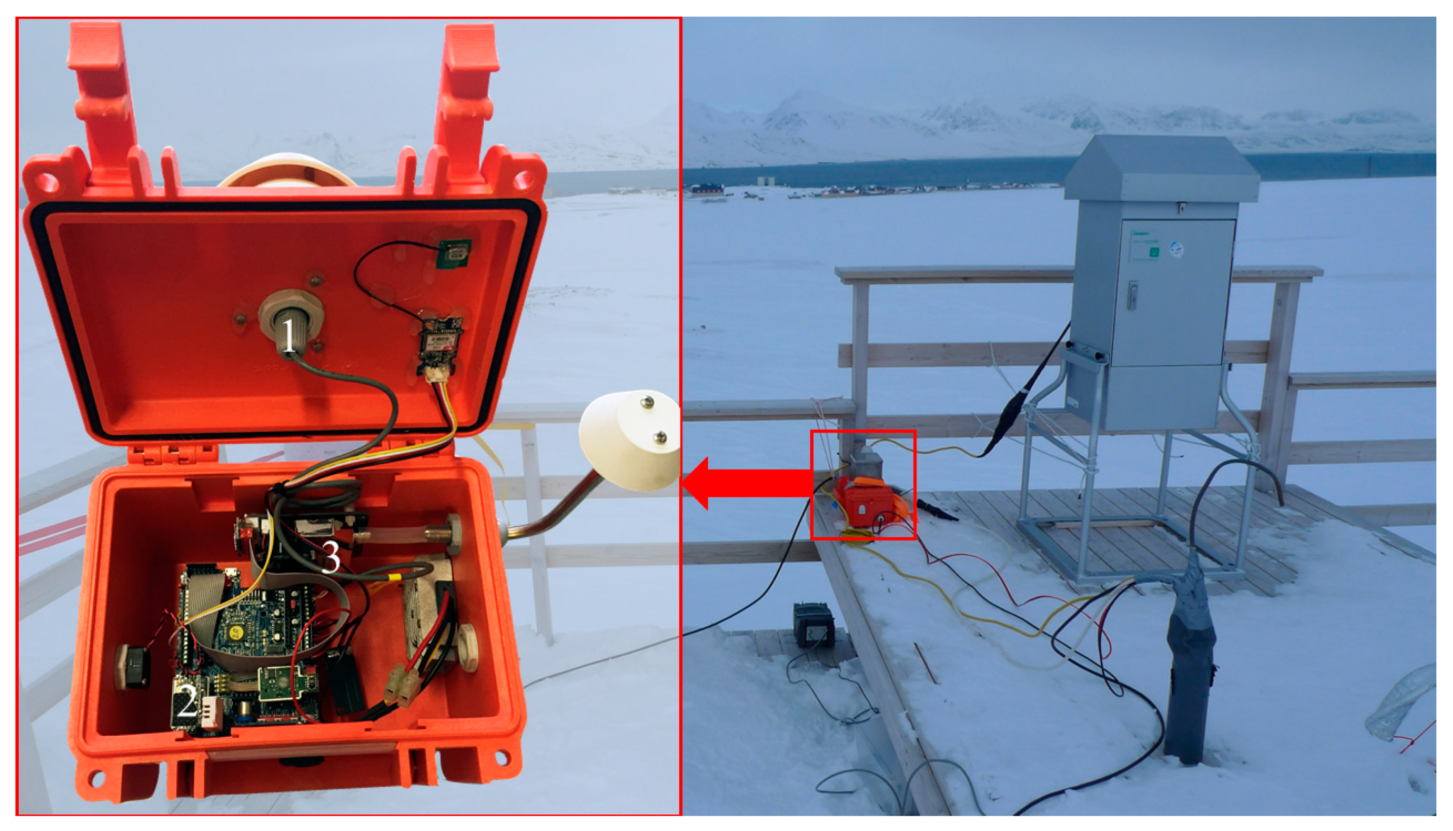
2.2. AIRQino Low-Cost Sensor
2.3. Reference Sensors at the CCT and GAL
2.4. Data Processing
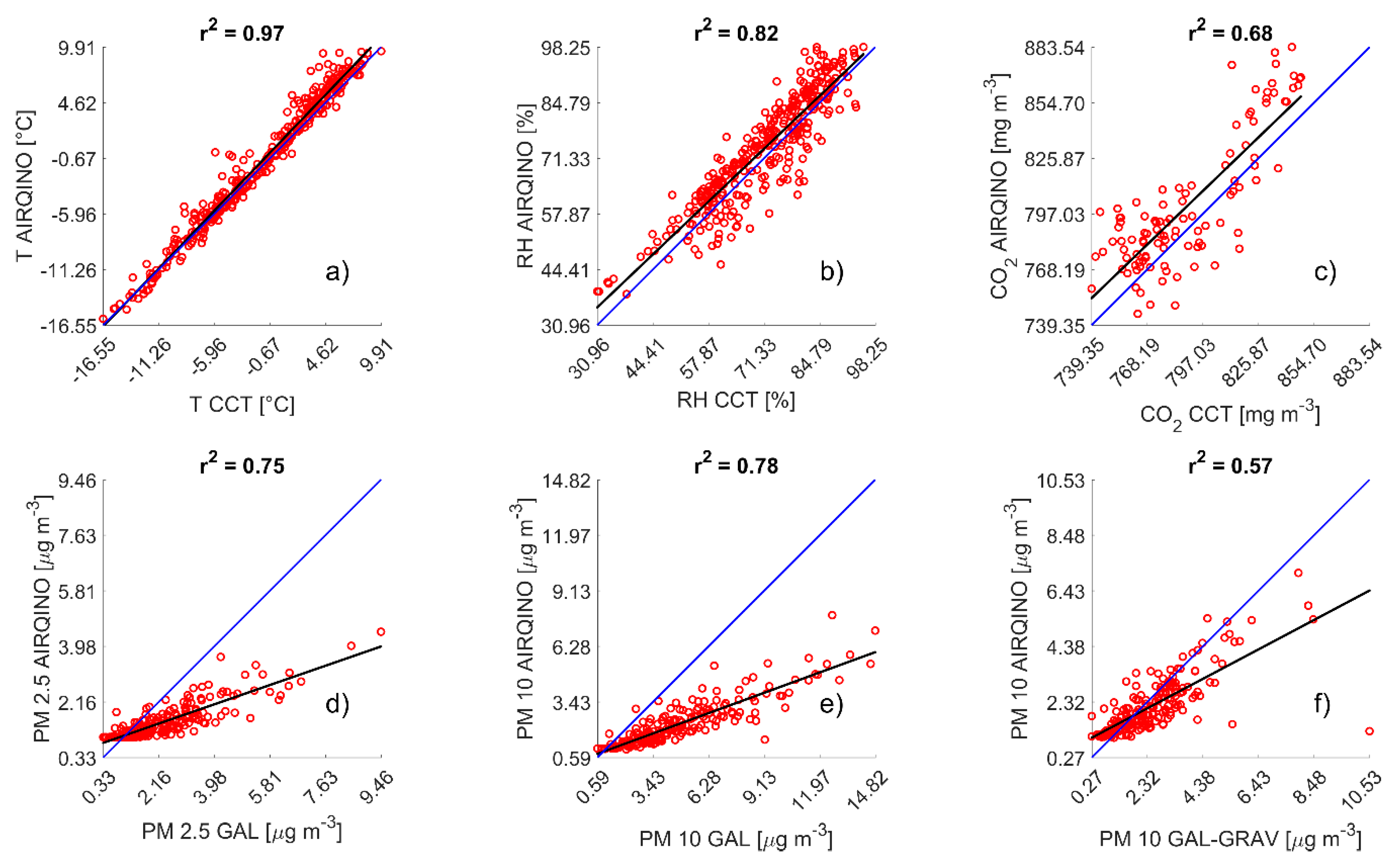
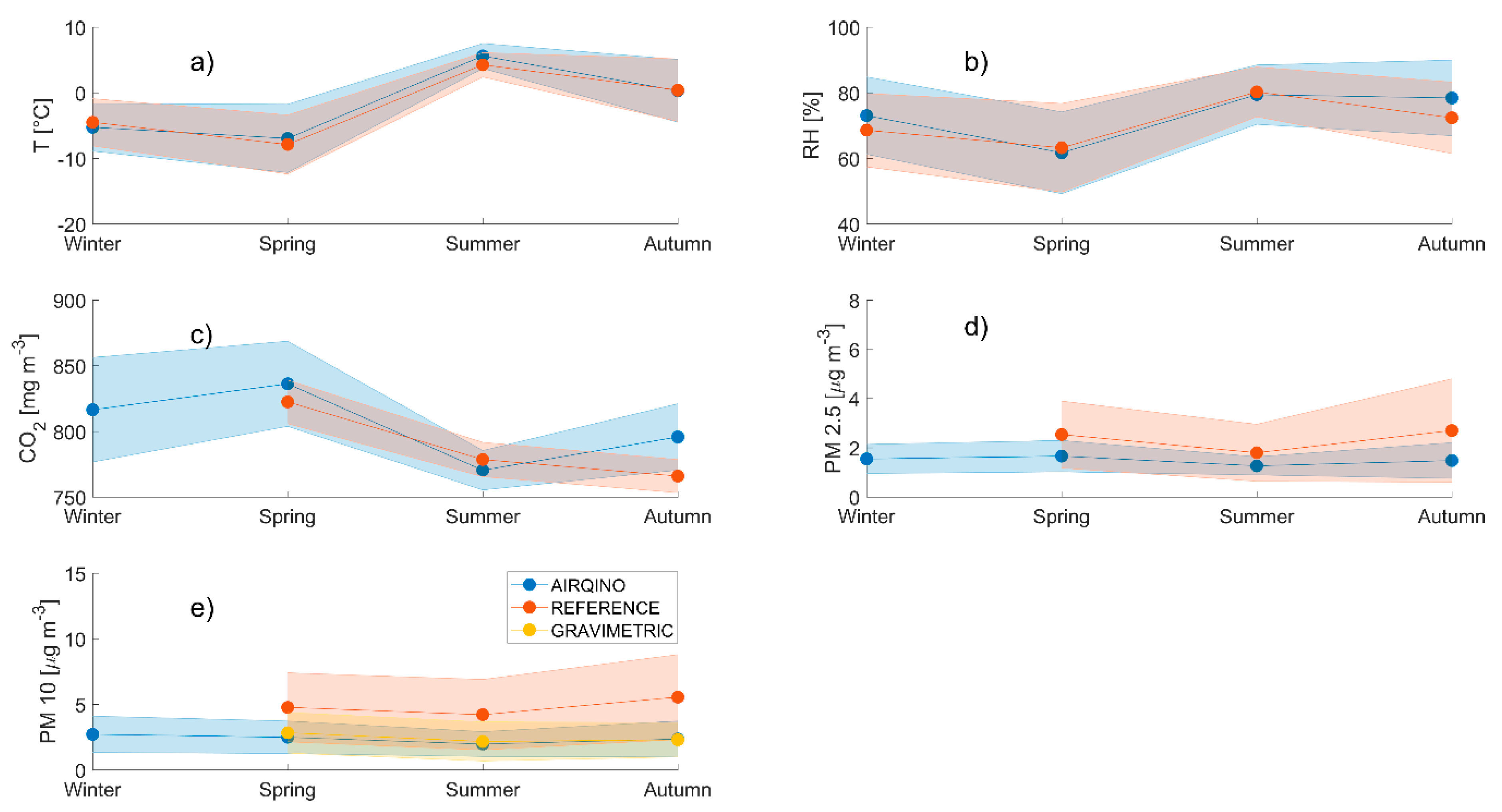
3. Results
4. Discussion
5. Conclusions
Author Contributions
Funding
Acknowledgments
Conflicts of Interest
References
- Holland, M.M.; Finnis, J.; Barrett, A.P.; Serreze, M.C. Projected changes in Arctic Ocean freshwater budgets. J. Geophys. Res. Space Phys. 2007, 112. [Google Scholar] [CrossRef]
- Serreze, M.C.; Barrett, A.P.; Stroeve, J.C.; Kindig, D.N.; Holland, M.M. The emergence of surface-based Arctic amplification. Cryosphere 2009, 3, 11–19. [Google Scholar] [CrossRef]
- Francis, J.; Skific, N. Evidence linking rapid Arctic warming to mid-latitude weather patterns. Philos. Trans. R. Soc. A Math. Phys. Eng. Sci. 2015, 373, 20140170. [Google Scholar] [CrossRef] [PubMed]
- Allen, M.R.; Dube, O.P.; Solecki, W.; Aragón-Durand, F.; Cramer, W.; Humphreys, S.; Kainuma, M.; Kala, J.; Mahowald, N.; Mulugetta, Y.; et al. In Global Warming of 1.5°C. 2018. Available online: https://www.ipcc.ch/sr15/download/ (accessed on 11 March 2020).
- Moore, G.W.K. The December 2015 North Pole Warming Event and the Increasing Occurrence of Such Events. Sci. Rep. 2016, 6, 39084. [Google Scholar] [CrossRef] [PubMed]
- Screen, J.; Simmonds, I.H. The central role of diminishing sea ice in recent Arctic temperature amplification. Nature 2010, 464, 1334–1337. [Google Scholar] [CrossRef]
- Cohen, J.; Screen, J.; Furtado, J.C.; Barlow, M.; Whittleston, D.; Coumou, D.; Francis, J.; Dethloff, K.; Entekhabi, D.; Overland, J.; et al. Recent Arctic amplification and extreme mid-latitude weather. Nat. Geosci. 2014, 7, 627–637. [Google Scholar] [CrossRef]
- Schuur, E.A.G.; McGuire, A.D.; Schadel, C.; Grosse, G.; Harden, J.; Hayes, D.J.; Hugelius, G.; Koven, C.D.; Kuhry, P.; Lawrence, D.M.; et al. Climate change and the permafrost carbon feedback. Nature 2015, 520, 171–179. [Google Scholar] [CrossRef]
- Oechel, W.; Laskowski, C.A.; Burba, G.; Gioli, B.; Kalhori, A.A.M. Annual patterns and budget of CO2flux in an Arctic tussock tundra ecosystem. J. Geophys. Res. Biogeosciences 2014, 119, 323–339. [Google Scholar] [CrossRef]
- Zona, D.; Gioli, B.; Commane, R.; Lindaas, J.; Wofsy, S.C.; Miller, C.E.; Dinardo, S.J.; Dengel, S.; Sweeney, C.; Karion, A.; et al. Cold season emissions dominate the Arctic tundra methane budget. Proc. Natl. Acad. Sci. 2015, 113, 40–45. [Google Scholar] [CrossRef]
- Goodrich, J.; Oechel, W.; Gioli, B.; Moreaux, V.; Murphy, P.C.; Burba, G.; Zona, D. Impact of different eddy covariance sensors, site set-up, and maintenance on the annual balance of CO2 and CH4 in the harsh Arctic environment. Agric. For. Meteorol. 2016, 228, 239–251. [Google Scholar] [CrossRef]
- Chong, C.-Y.; Kumar, S. Sensor networks: Evolution, opportunities, and challenges. Proc. IEEE 2003, 91, 1247–1256. [Google Scholar] [CrossRef]
- Kumar, P.; Morawska, L.; Martani, C.; Biskos, G.; Neophytou, M.K.-A.; Di Sabatino, S.; Bell, M.; Norford, L.; Britter, R. The rise of low-cost sensing for managing air pollution in cities. Environ. Int. 2015, 75, 199–205. [Google Scholar] [CrossRef] [PubMed]
- Schneider, P.; Castell, N.; Vogt, M.; Dauge, F.R.; Lahoz, W.A.; Bartonova, A. Mapping urban air quality in near real-time using observations from low-cost sensors and model information. Environ. Int. 2017, 106, 234–247. [Google Scholar] [CrossRef] [PubMed]
- Motlagh, N.H.; Petaja, T.; Kulmala, M.; Trachoma, S.; Lagerspetz, E.; Nurmi, P.; Li, X.; Varjonen, S.; Mineraud, J.; Siekkinen, M.; et al. Toward Massive Scale Air Quality Monitoring. IEEE Commun. Mag. 2020, 58, 54–59. [Google Scholar] [CrossRef]
- Snyder, E.G.; Watkins, T.H.; Solomon, P.A.; Thoma, E.D.; Williams, R.W.; Hagler, G.; Shelow, D.; Hindin, D.A.; Kilaru, V.; Preuss, P.W. The Changing Paradigm of Air Pollution Monitoring. Environ. Sci. Technol. 2013, 47, 11369–11377. [Google Scholar] [CrossRef] [PubMed]
- Piermattei, V.; Madonia, A.; Bonamano, S.; Martellucci, R.; Bruzzone, G.; Ferretti, R.; Odetti, A.; Azzaro, M.; Zappalà, G.; Marcelli, M. Cost-Effective Technologies to Study the Arctic Ocean Environment. Sensors 2018, 18, 2257. [Google Scholar] [CrossRef] [PubMed]
- Pasquali, V.; D’Alessandro, G.; Gualtieri, R.; Leccese, F. A new data logger based on Raspberry-Pi for Arctic Notostraca locomotion investigations. Measurement 2017, 110, 249–256. [Google Scholar] [CrossRef]
- Gagnon, S.; L’Hérault, E.; Lemay, M.; Allard, M. New low-cost automated system of closed chambers to measure greenhouse gas emissions from the tundra. Agric. For. Meteorol. 2016, 228, 29–41. [Google Scholar] [CrossRef]
- Kottek, M.; Grieser, J.; Beck, C.; Rudolf, B.; Rubel, F. World Map of the Köppen-Geiger climate classification updated. Meteorol. Z. 2006, 15, 259–263. [Google Scholar] [CrossRef]
- Mazzola, M.; Viola, A.P.; Lanconelli, C.; Vitale, V. Atmospheric observations at the Amundsen-Nobile Climate Change Tower in Ny-Ålesund, Svalbard. RENDICONTI Lince- 2016, 27, 7–18. [Google Scholar] [CrossRef]
- Udisti, R.; Bazzano, A.; Becagli, S.; Bolzacchini, E.; Caiazzo, L.; Cappelletti, D.; Ferrero, L.; Frosini, D.; Giardi, F.; Grotti, M.; et al. Sulfate source apportionment in the Ny-Ålesund (Svalbard Islands) Arctic aerosol. RENDICONTI Lince- 2016, 27, 85–94. [Google Scholar] [CrossRef]
- Cavaliere, A.; Carotenuto, F.; Di Gennaro, S.F.; Gioli, B.; Gualtieri, G.; Martelli, F.; Matese, A.; Toscano, P.; Vagnoli, C.; Zaldei, A.; et al. Development of Low-Cost Air Quality Stations for Next Generation Monitoring Networks: Calibration and Validation of PM2.5 and PM10 Sensors. Sensors 2018, 18, 2843. [Google Scholar] [CrossRef] [PubMed]
- Giardi, F.; Becagli, S.; Traversi, R.; Frosini, D.; Severi, M.; Caiazzo, L.; Ancillotti, C.; Cappelletti, D.; Moroni, B.; Grotti, M.; et al. Size distribution and ion composition of aerosol collected at Ny-Ålesund in the spring–summer field campaign 2013. RENDICONTI Lince- 2016, 27, 47–58. [Google Scholar] [CrossRef]
- Lupi, A.; Busetto, M.; Becagli, S.; Giardi, F.; Lanconelli, C.; Mazzola, M.; Udisti, R.; Hansson, H.-C.; Henning, T.; Petkov, B.; et al. Multi-seasonal ultrafine aerosol particle number concentration measurements at the Gruvebadet observatory, Ny-Ålesund, Svalbard Islands. RENDICONTI Lince- 2016, 27, 59–71. [Google Scholar] [CrossRef]
- Yanosky, J.D.; Maclntosh, D.L. A Comparison of Four Gravimetric Fine Particle Sampling Methods. J. Air Waste Manag. Assoc. 2001, 51, 878–884. [Google Scholar] [CrossRef]
- Saarikoski, S.; Mäkelä, T.; Hillamo, R.M.; Aalto, P.P.; Kerminen, V.-M.; Kulmala, M. Physico-chemical characterization and mass closure of size-segregated atmospheric aerosols in Hyytiälä, Finland. Boreal Env. Res. 2005, 10, 385–400. [Google Scholar]
- Viskari, T.; Asmi, E.; Virkkula, A.; Kolmonen, P.; Petäjä, T.; Järvinen, H. Estimation of aerosol particle number distribution with Kalman Filtering – Part 2: Simultaneous use of DMPS, APS and nephelometer measurements. Atmospheric Chem. Phys. Discuss. 2012, 12, 11781–11793. [Google Scholar] [CrossRef]
- Asmi, E.; Kondratyev, V.; Brus, D.; Laurila, T.; Lihavainen, H.; Backman, J.; Vakkari, V.; Aurela, M.; Hatakka, J.; Viisanen, Y.; et al. Aerosol size distribution seasonal characteristics measured in Tiksi, Russian Arctic. Atmospheric Chem. Phys. Discuss. 2016, 16, 1271–1287. [Google Scholar] [CrossRef]
- Maturilli, M.; Herber, A.; König-Langlo, G. Climatology and time series of surface meteorology in Ny-Ålesund, Svalbard. Earth Syst. Sci. Data 2013, 5, 155–163. [Google Scholar] [CrossRef]
- Lloyd, C.R. On the physical controls of the carbon dioxide balance at a high Arctic site in Svalbard. Theor. Appl. Clim. 2001, 70, 167–182. [Google Scholar] [CrossRef]
- Ciais, P.; Sabine, C.; Bala, G.; Bopp, L.; Brovkin, V.; Canadell, J.; Chhabra, A.; DeFries, R.; Galloway, J.; Heimann, M.; et al. Carbon and Other Biogeochemical Cycles. In Climate Change 2013: The Physical Science Basis. Contribution of Working Group I to the Fifth Assessment Report of the Intergovernmental Panel on Climate Change; Stocker, T.F., Qin, D., Plattner, G.-K., Tignor, M., Allen, S.K., Boschung, J., Nauels, A., Xia, Y., Bex, V., Midgley, P.M., Eds.; Cambridge University Press: Cambridge, UK; New York, NY, USA, 2013; pp. 465–470. [Google Scholar]
- Moroni, B.; Becagli, S.; Bolzacchini, E.; Busetto, M.; Cappelletti, D.; Crocchianti, S.; Ferrero, L.; Frosini, D.; Lanconelli, C.; Lupi, A.; et al. Vertical Profiles and Chemical Properties of Aerosol Particles upon Ny-Ålesund (Svalbard Islands). Adv. Meteorol. 2015, 2015, 1–11. [Google Scholar] [CrossRef]
- Becagli, S.; Lazzara, L.; Marchese, C.; Dayan, U.; Ascanius, S.; Cacciani, M.; Caiazzo, L.; DiBiagio, C.; Di Iorio, T.; Di Sarra, A.; et al. Relationships linking primary production, sea ice melting, and biogenic aerosol in the Arctic. Atmospheric Environ. 2016, 136, 1–15. [Google Scholar] [CrossRef]
- Liu, H.-Y.; Schneider, P.; Haugen, R.; Vogt, M. Performance Assessment of a Low-Cost PM2.5 Sensor for a near Four-Month Period in Oslo, Norway. Atmosphere 2019, 10, 41. [Google Scholar] [CrossRef]
- Ioakimidis, C.S.; Galatoulas, N.-F.; Dallas, P.I.; Ibarra, L.M.C.; Margaritis, D.; Ioakimidis, C.S. Development and On-Field Testing of Low-Cost Portable System for Monitoring PM2.5 Concentrations. Sensors 2018, 18, 1056. [Google Scholar]
- Badura, M.; Batog, P.; Drzeniecka-Osiadacz, A.; Modzel, P. Evaluation of Low-Cost Sensors for Ambient PM2.5 Monitoring. J. Sensors 2018, 2018, 1–16. [Google Scholar] [CrossRef]
- Hapidin, D.A.; Saputra, C.; Maulana, D.S.; Munir, M.M.; Khairurrijal, K. Aerosol Chamber Characterization for Commercial Particulate Matter (PM) Sensor Evaluation. Aerosol Air Qual. Res. 2019, 19, 181–194. [Google Scholar] [CrossRef]
- Nava, S.; Lucarelli, F.; Amato, F.; Becagli, S.; Calzolai, G.; Chiari, M.; Giannoni, M.; Traversi, R.; Udisti, R. Biomass burning contributions estimated by synergistic coupling of daily and hourly aerosol composition records. Sci. Total. Environ. 2015, 511, 11–20. [Google Scholar] [CrossRef]
- Zieger, P.; Fierz-Schmidhauser, R.; Weingartner, E.; Baltensperger, U. Effects of relative humidity on aerosol light scattering: results from different European sites. Atmospheric Chem. Phys. Discuss. 2013, 13, 10609–10631. [Google Scholar] [CrossRef]
- Li, H.; Zhu, Y.; Zhao, Y.; Chen, T.; Jiang, Y.; Shan, Y.; Liu, Y.; Mu, J.; Yin, X.; Wu, D.; et al. Evaluation of the Performance of Low-Cost Air Quality Sensors at a High Mountain Station with Complex Meteorological Conditions. Atmosphere 2020, 11, 212. [Google Scholar] [CrossRef]
- Knepp, T.N.; Bottenheim, J.; Carlsén, M.; Carlson, D.; Donohoue, D.; Friederich, G.; Matrai, P.A.; Netcheva, S.; Perovich, D.K.; Santini, R.; et al. Development of an autonomous sea ice tethered buoy for the study of ocean-atmosphere-sea ice-snow pack interactions: the O-buoy. Atmospheric Meas. Tech. 2010, 3, 249–261. [Google Scholar] [CrossRef]
- Ishibashi, S.; Aoki, T.; Tsukioka, S.; Yoshida, H.; Inada, T.; Kabeno, T.; Maeda, T.; Hirokawa, K.; Yokoyama, K.; Tani, T.; et al. An ocean going autonomous underwater vehicle “URASHIMA” equipped with a fuel cell. In Proceedings of the 2004 International Symposium on Underwater Technology (IEEE Cat. No.04EX869), Taipei, Taiwan, 20–23 April 2004; pp. 209–214. [Google Scholar]
- Dai, Z.; Xu, L.; Duan, G.; Li, T.; Zhang, H.; Li, Y.; Wang, Y.; Wang, Y.; Cai, W. Fast-Response, Sensitivitive and Low-Powered Chemosensors by Fusing Nanostructured Porous Thin Film and IDEs-Microheater Chip. Sci. Rep. 2013, 3, 1669. [Google Scholar] [CrossRef] [PubMed]
- Dai, Z.; Liang, T.; Lee, J.-H. Gas sensors using ordered macroporous oxide nanostructures. Nanoscale Adv. 2019, 1, 1626–1639. [Google Scholar] [CrossRef]


| Variable | Units | Instrument | Minimum | Average | Maximum | Comparison Statistics | |||
|---|---|---|---|---|---|---|---|---|---|
| r2 (p) | RMSE | Bias | Norm. Bias | ||||||
| T | °C | AIRQino | −16.22 | −1.50 | 9.52 | 0.97 (<0.05) | 1.17 | 0.48 | 0.18 % |
| CCT | −16.55 | −1.74 | 9.91 | ||||||
| RH | % | AIRQino | 38.47 | 73.16 | 98.25 | 0.82 (<0.05) | 6.04 | 2.32 | 3.21 % |
| CCT | 30.96 | 71.35 | 95.38 | ||||||
| CO2 | mg m−3 | AIRQino | 735.85 | 803.44 | 911.29 | 0.68 (<0.05) | 23.13 | 12.15 | 1.53 % |
| CCT | 739.35 | 789.90 | 847.82 | ||||||
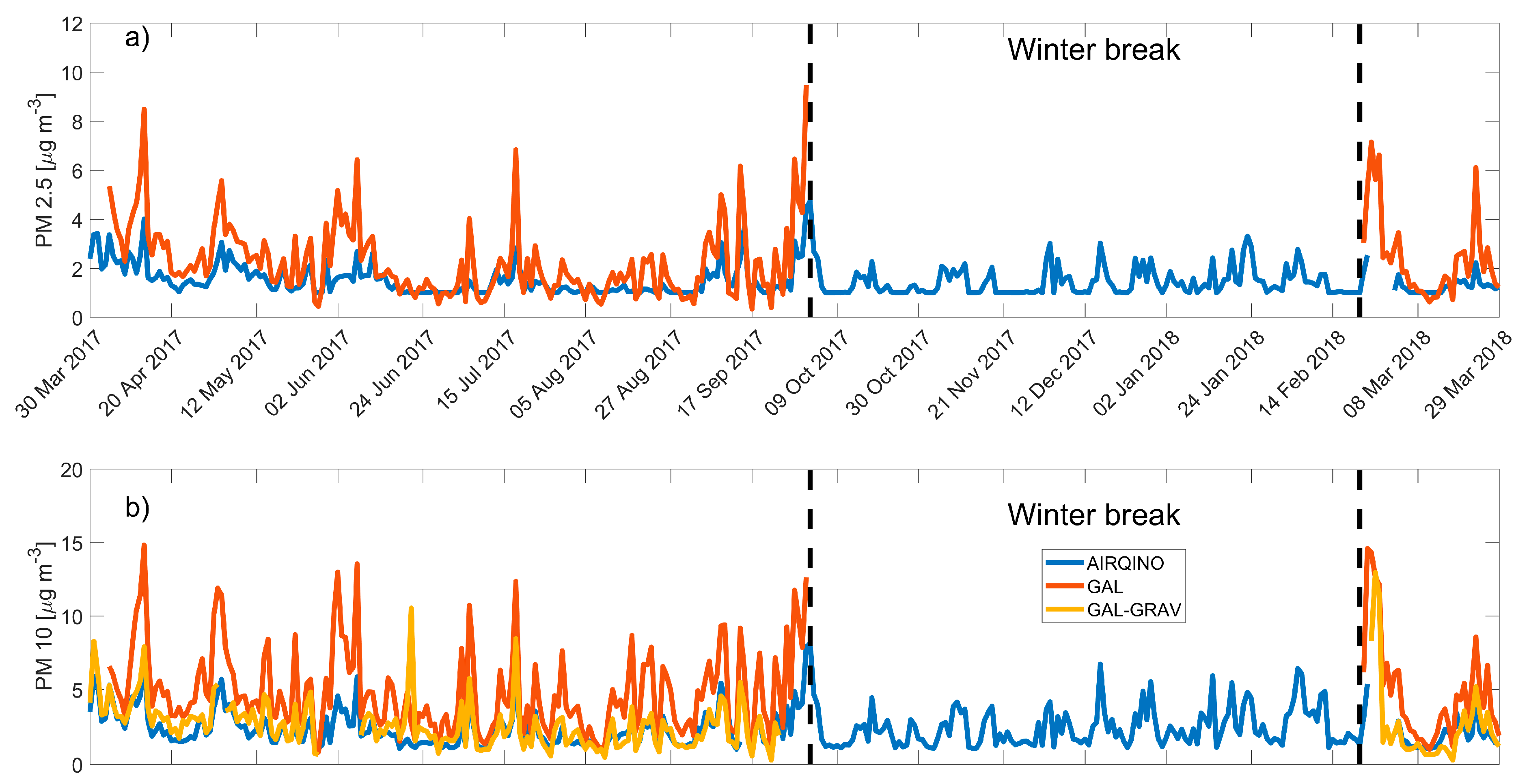
| PM2.5 | µg m−3 | AIRQino | 1.00 | 1.48 | 4.73 | 0.75 (<0.05) | 1.27 | -0.77 | −42.40 % |
| GAL | 0.33 | 2.31 | 9.46 | ||||||
| PM10 | µg m−3 | AIRQino | 1.00 | 2.37 | 8.14 | 0.78 (<0.05) | 3.06 | -2.40 | −73.42 % |
| GAL | 0.59 | 4.81 | 14.82 | ||||||
| GAL-GRAV | 0.27 | 2.59 | 12.95 | 0.57 (<0.05) | 1.04 | -0.31 | −13.24% | ||
© 2020 by the authors. Licensee MDPI, Basel, Switzerland. This article is an open access article distributed under the terms and conditions of the Creative Commons Attribution (CC BY) license (http://creativecommons.org/licenses/by/4.0/).
Share and Cite
Carotenuto, F.; Brilli, L.; Gioli, B.; Gualtieri, G.; Vagnoli, C.; Mazzola, M.; Viola, A.P.; Vitale, V.; Severi, M.; Traversi, R.; et al. Long-Term Performance Assessment of Low-Cost Atmospheric Sensors in the Arctic Environment. Sensors 2020, 20, 1919. https://doi.org/10.3390/s20071919
Carotenuto F, Brilli L, Gioli B, Gualtieri G, Vagnoli C, Mazzola M, Viola AP, Vitale V, Severi M, Traversi R, et al. Long-Term Performance Assessment of Low-Cost Atmospheric Sensors in the Arctic Environment. Sensors. 2020; 20(7):1919. https://doi.org/10.3390/s20071919
Chicago/Turabian StyleCarotenuto, Federico, Lorenzo Brilli, Beniamino Gioli, Giovanni Gualtieri, Carolina Vagnoli, Mauro Mazzola, Angelo Pietro Viola, Vito Vitale, Mirko Severi, Rita Traversi, and et al. 2020. "Long-Term Performance Assessment of Low-Cost Atmospheric Sensors in the Arctic Environment" Sensors 20, no. 7: 1919. https://doi.org/10.3390/s20071919
APA StyleCarotenuto, F., Brilli, L., Gioli, B., Gualtieri, G., Vagnoli, C., Mazzola, M., Viola, A. P., Vitale, V., Severi, M., Traversi, R., & Zaldei, A. (2020). Long-Term Performance Assessment of Low-Cost Atmospheric Sensors in the Arctic Environment. Sensors, 20(7), 1919. https://doi.org/10.3390/s20071919