Spurious Absorption Frequency Appearance Due to Frequency Conversion Processes in Pulsed THz TDS Problems


Abstract
1. Literature review and introduction
2. Theoretical Analysis
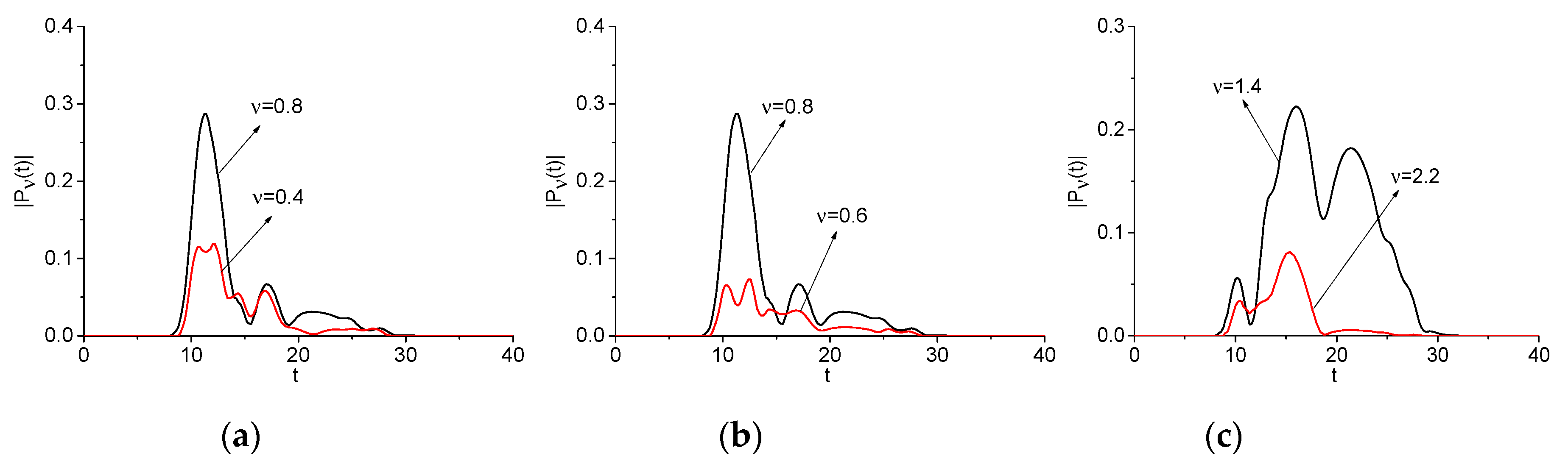
2.1. Frequency Conversion Near the Spectral Maximum of Artificial Signals
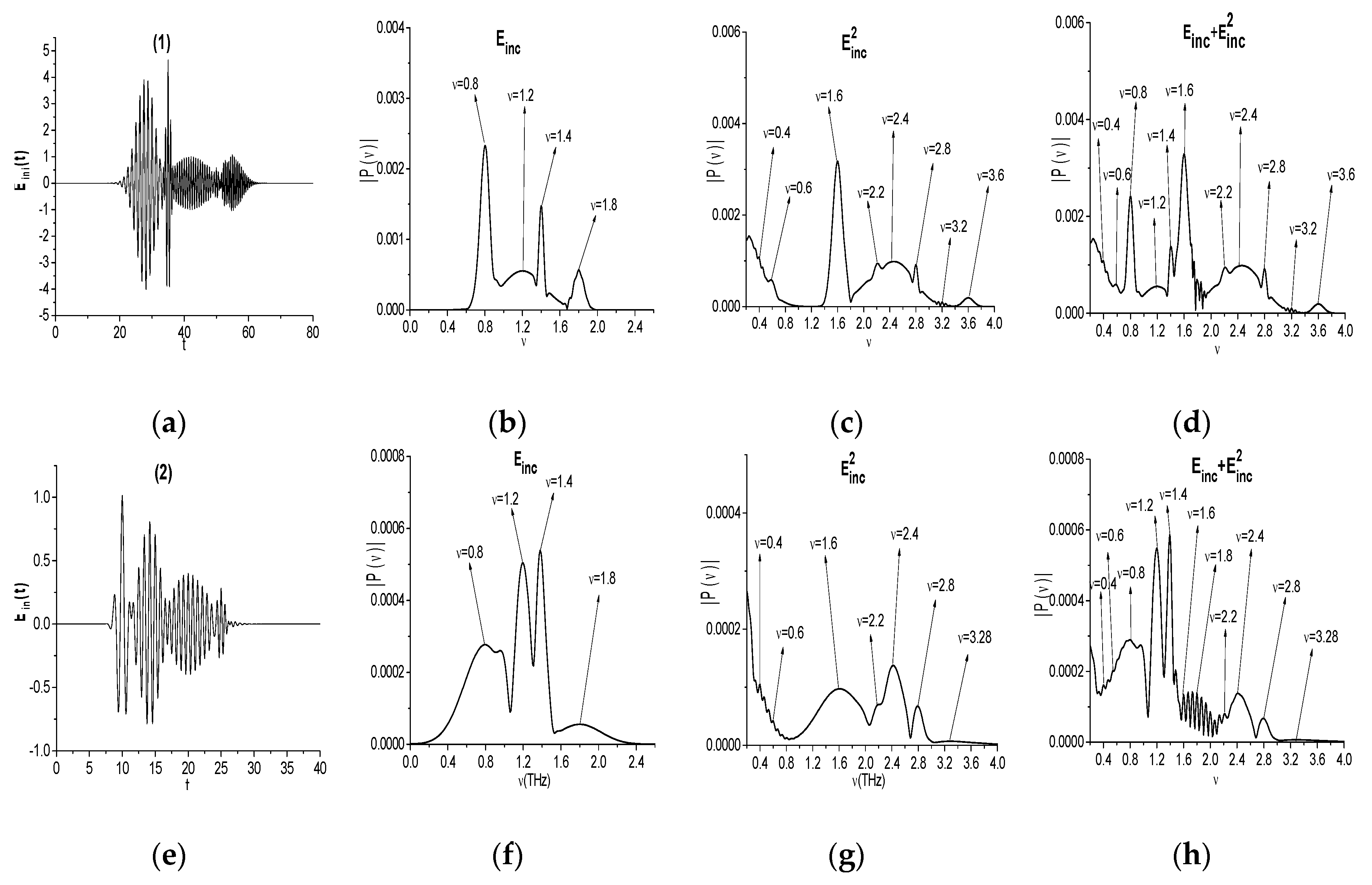
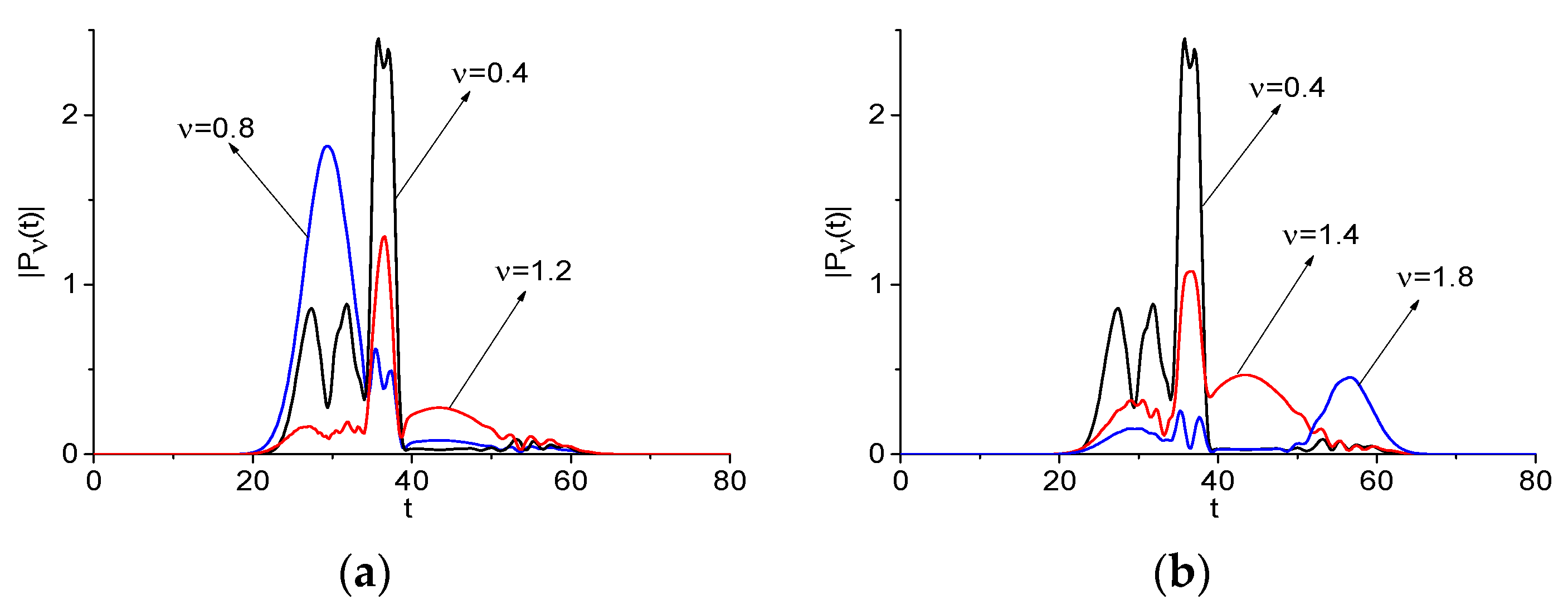
2.1.1. Correlation between the Spectral Line Dynamics at the Basic and Doubled Frequencies for the Signal Consisting of Sub-Pulses with Three Narrow Spectra and One Broad Spectrum (Example 1)
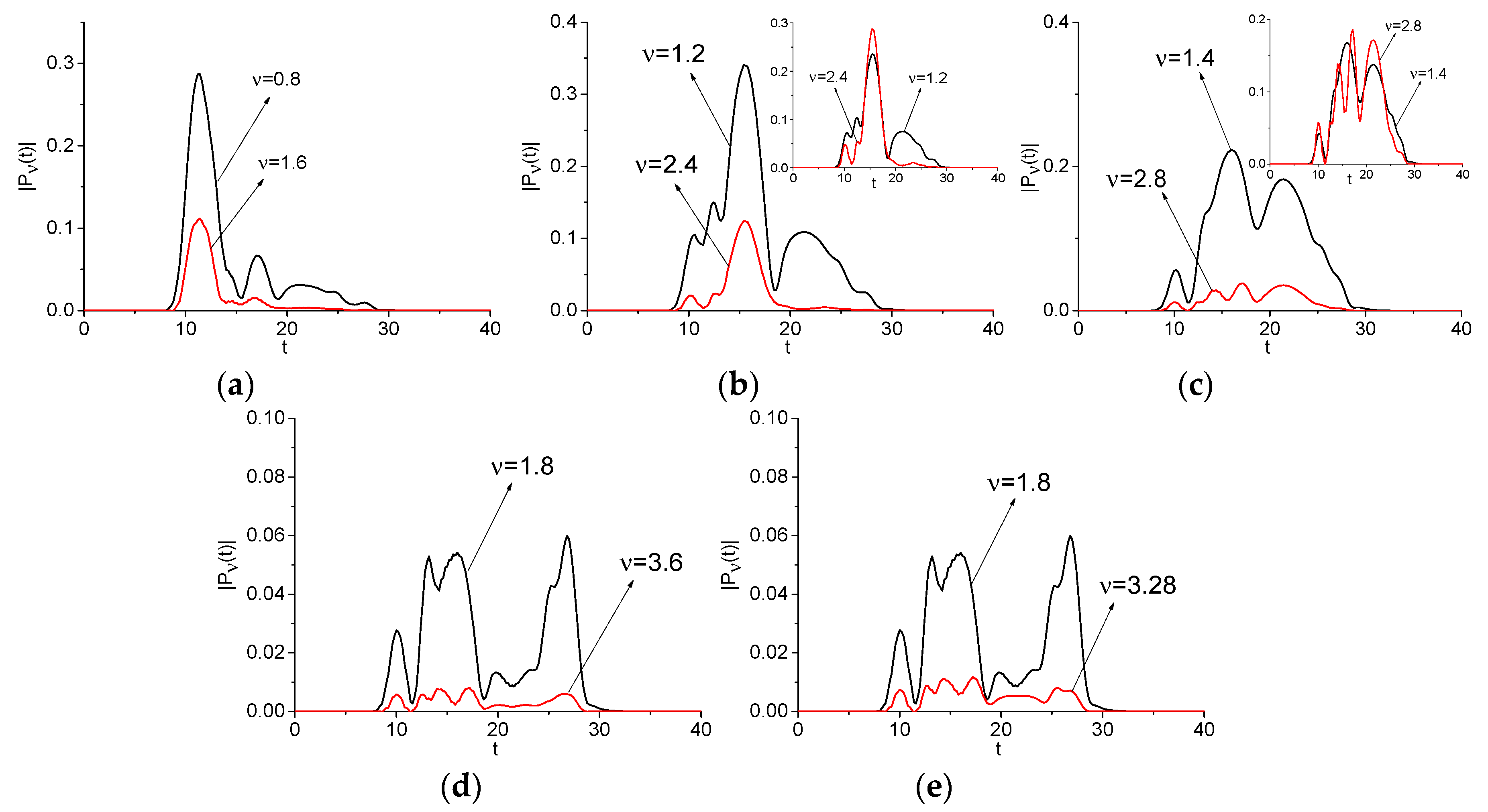
2.1.2. Correlation between the Spectral Line Dynamics at the Basic and Doubled Frequencies for the Signal Consisting of Sub-Pulses with Three Broad Spectra and One Narrow Spectrum (Example 2)
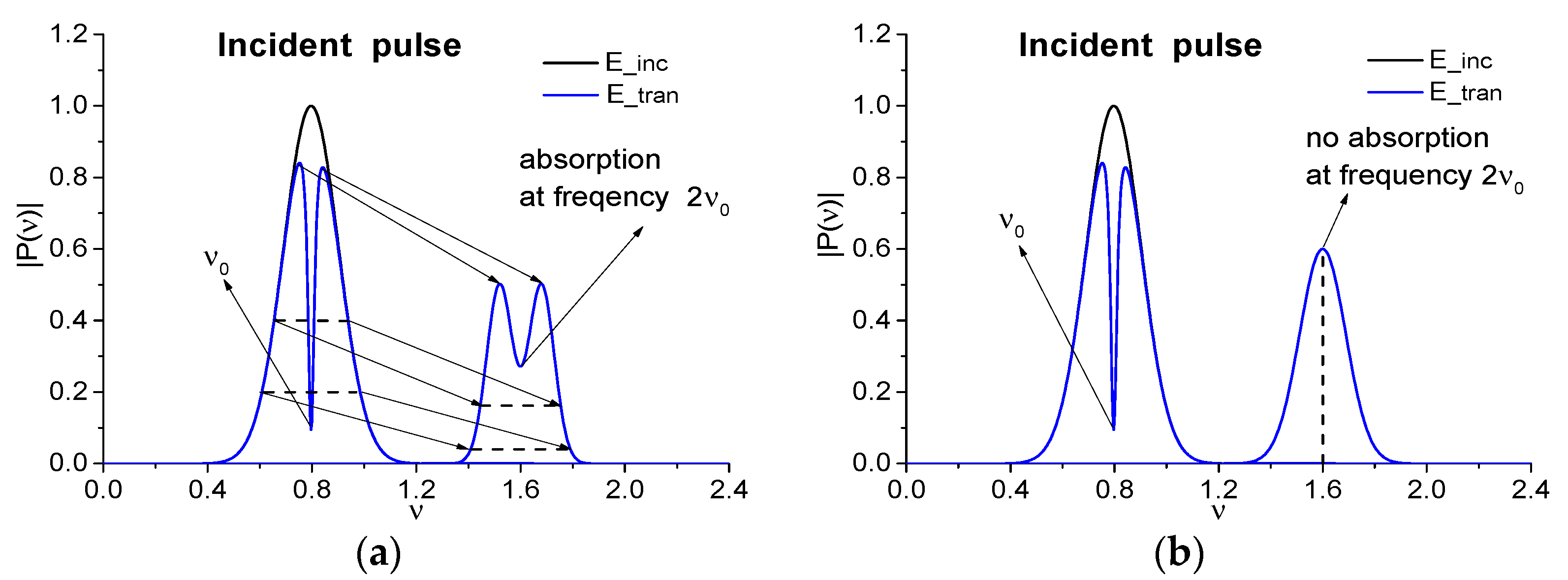
2.2. Frequency Conversion Near Minimum of the Pulse Spectrum
2.2.1. The Artificial Signals Consisting from the Sub-Pulses (Examples 1 and 2)
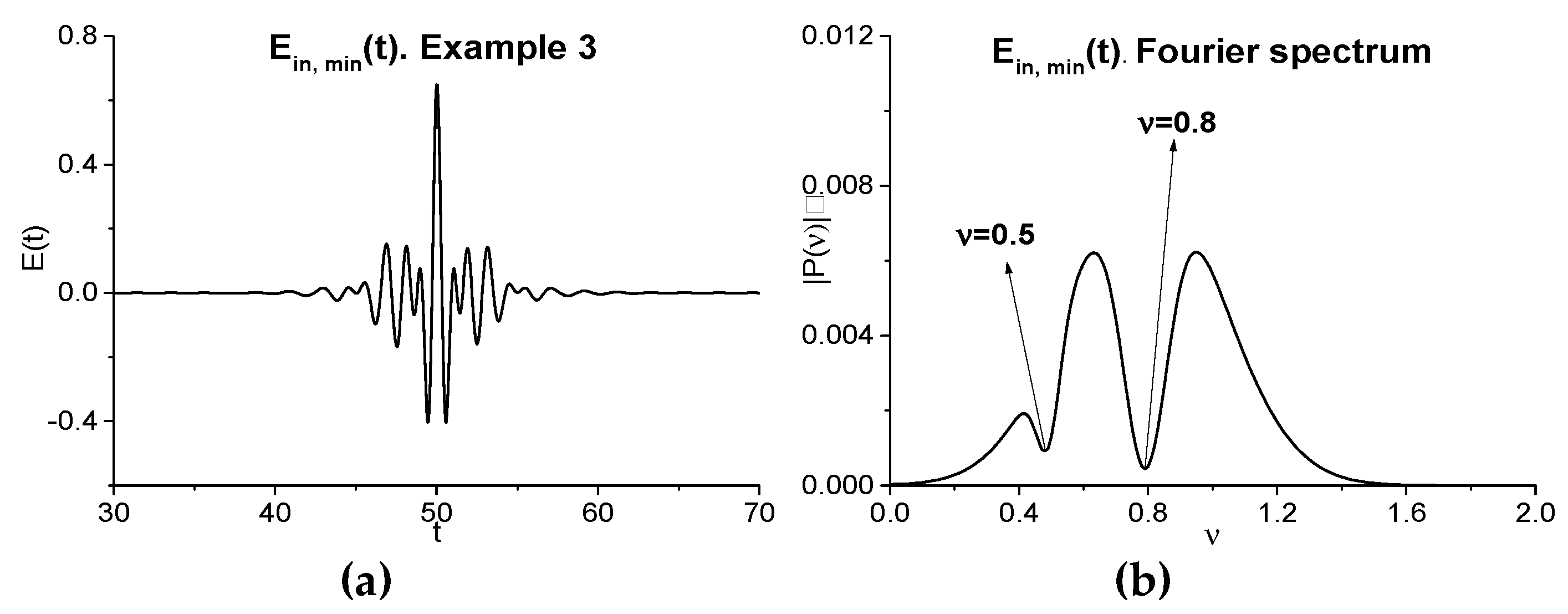
2.2.2. Artificial Signal without Sub-Pulse Structure (Example 3)
3. Experimental Setups
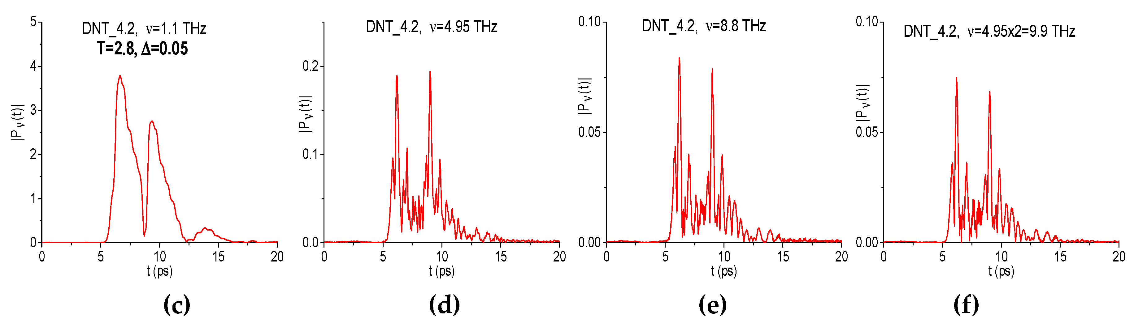
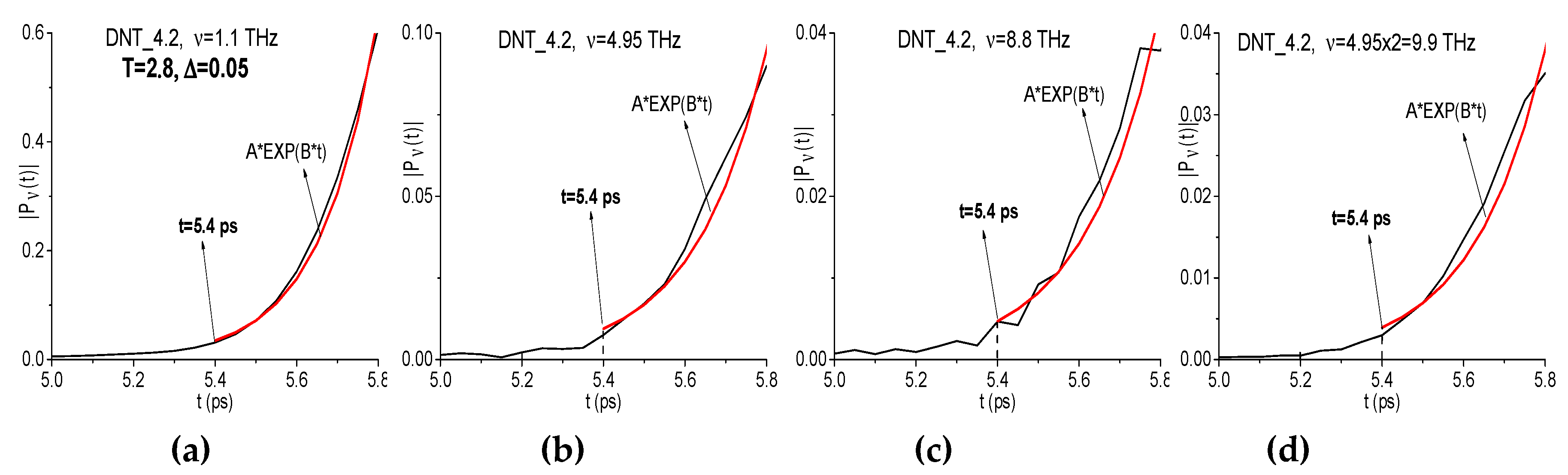
4. Results of the Experiment Using a Broadband THz Pulse
- RDX: ν = 0.82, 1.05, 1.50, 1.96, 2.20, 3.08, 6.73, 10.35, 11.34, 12.33, 13.86, 14.52, 17.74, 18.12, 20.13 THz
- HMX: ν = 1.78, 2.51, 2.82, 5.31, 6.06, 11.28, 12.00, 12.54, 12.96, 13.74, 14.55, 18.15, 18.60, 19.38 THz;
- 2,4-DNT: ν = 0.45, 0.66, 1.08, 2.52, 4.98, 8.88, 10.56, 11.58, 12.81, 14.34, 15.69, 19.05, 20.04 THz; and,
- 2,6-DNT: ν = 1.10, 1.35, 1.56, 2.50, 5.61, 6.75, 9.78, 11.43, 13.32, 13.89, 15.39, 17.25 THz.
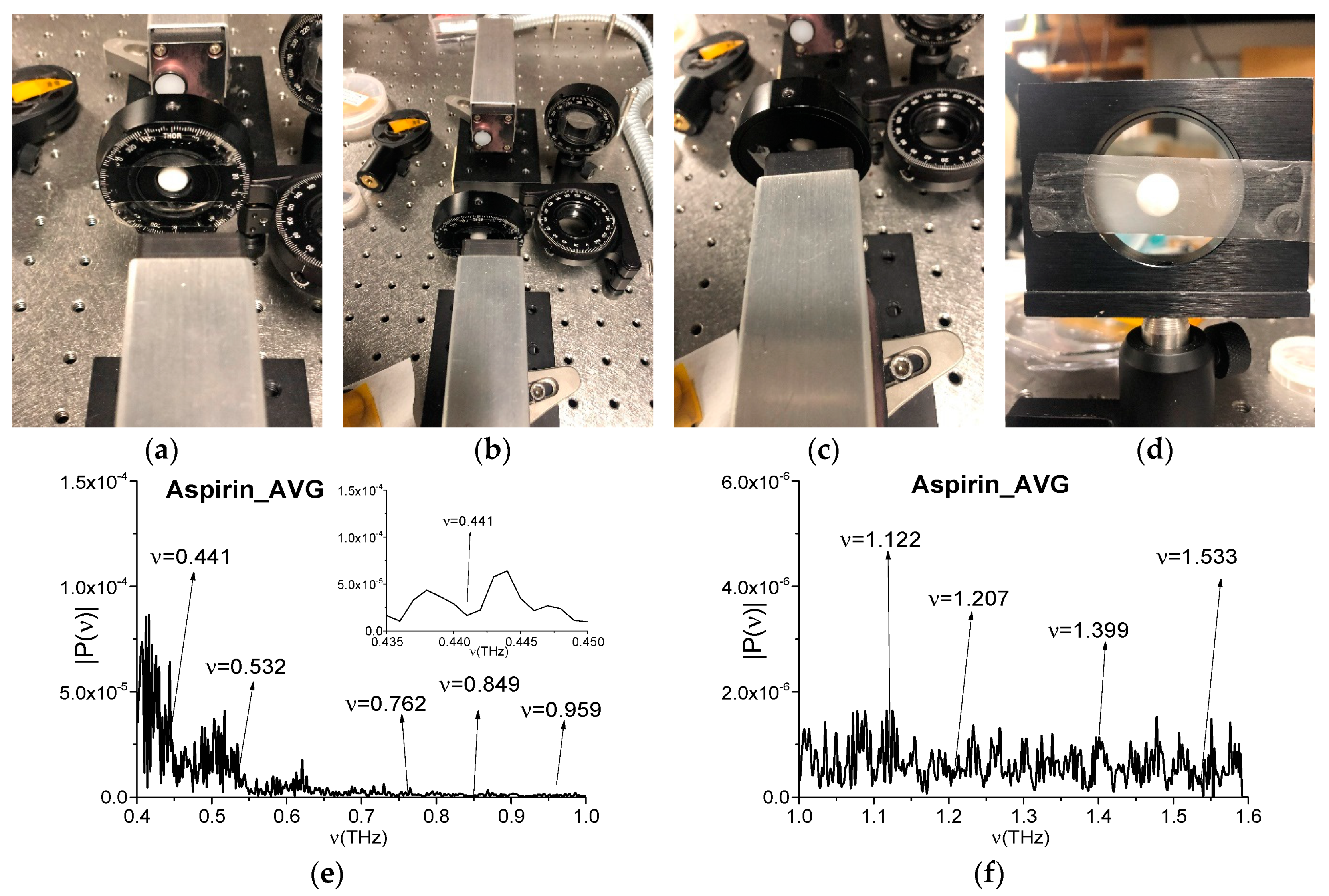
5. Results of the Experiment Using a Narrowband CW THz Radiation
5.1. Aspirin Pellet
5.2. Piece of Soap
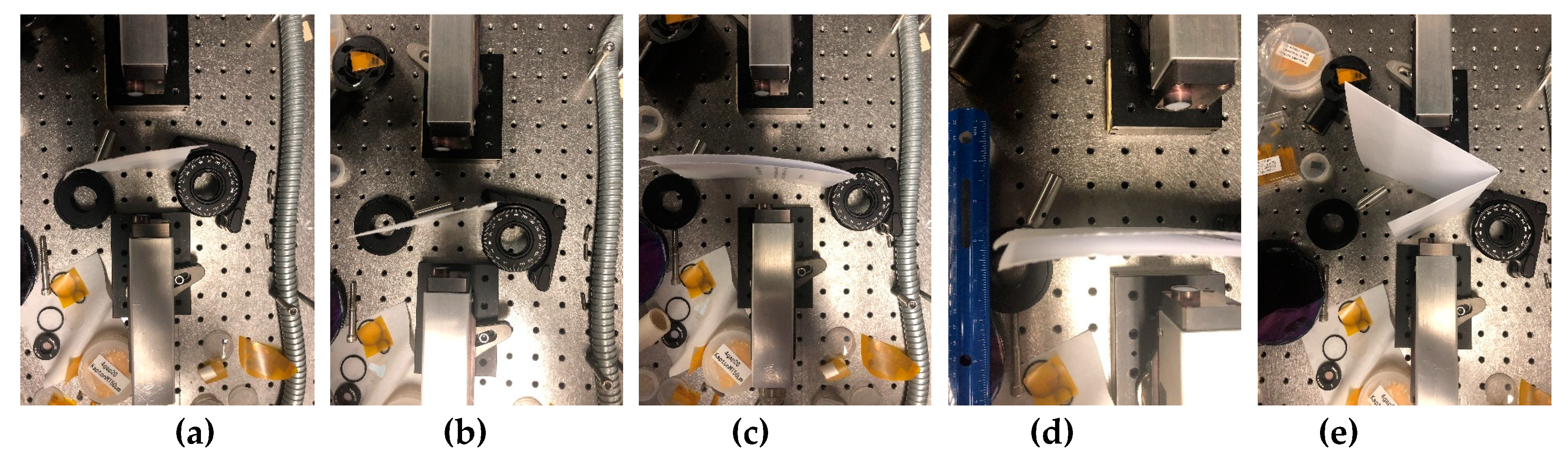
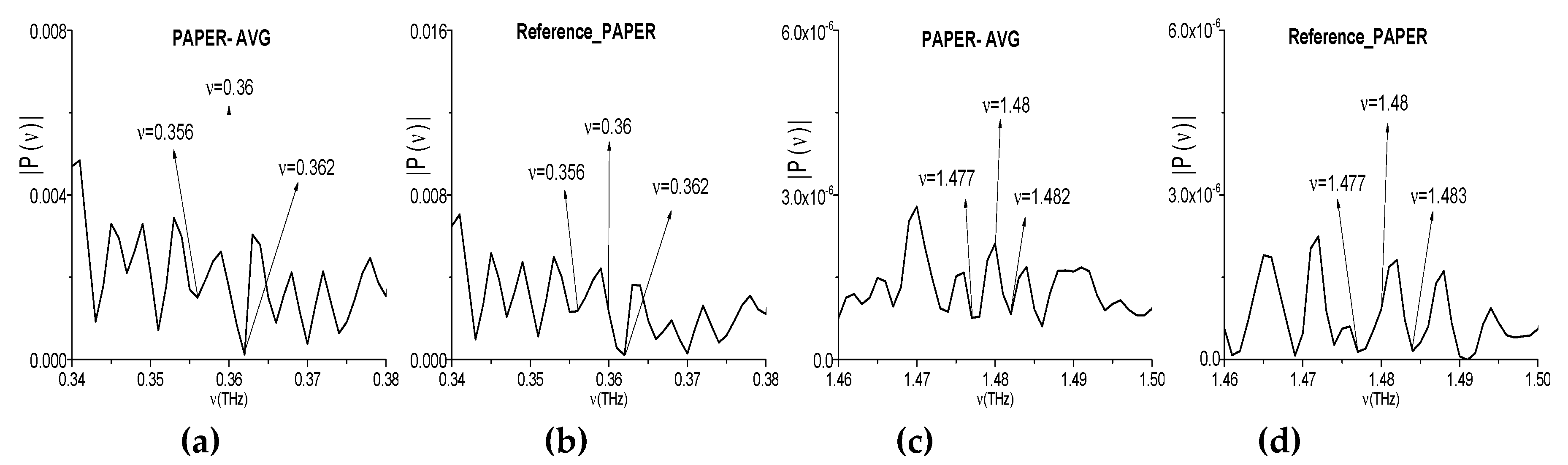
5.3. Sheet of Paper
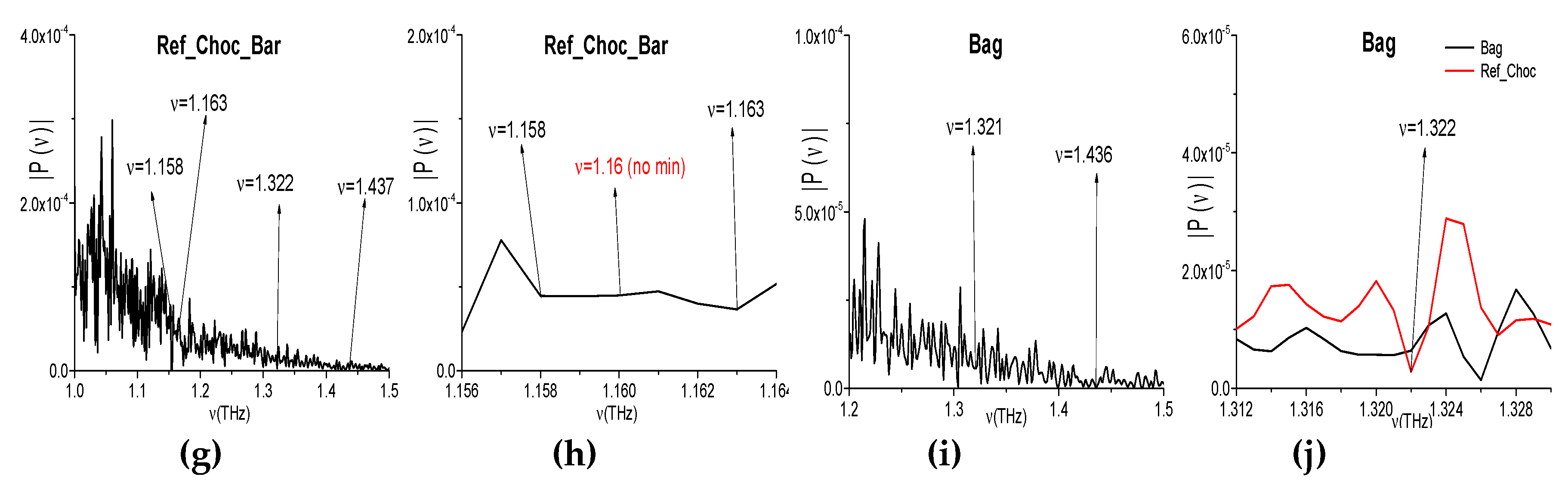
5.4. Polyethylene Bag
5.5. Chocolate Bar
6. Conclusions
Author Contributions
Acknowledgments
Conflicts of Interest
Appendix A. Fourier–Gabor Window Transform
Appendix B. Computation of the Integral Spectral Intensity Using the Time-Dependent Spectral Brightness


 | 0.7 | 0.9 | 1.05 | |||
| 0.05 | 3.975·10−2 | 4.319·10−3 | 2.006·10−2 | |||
| 0.05 | 3.989·10−2 | 4.276·10−3 | 2.000·10−2 | |||
| 0.01 | 3.981·10−2 | 4.284·10−3 | 2.003·10−2 | |||
Appendix C. Influence of Window Shift on the Accuracy of Constructing Spectral Line Dynamics


References
- Federici, J.F.; Schulkin, B.; Huang, F.; Gary, D.; Barat, R.; Oliveira, F.; Zimdars, D. THz imaging and sensing for security applications—Explosives, weapons and drugs. Semicond. Sci. Technol. 2005, 20, S266–S280. [Google Scholar] [CrossRef]
- Leahy-Hoppa, M.R.; Fitch, M.J.; Zheng, X.; Hayden, L.M.; Osiander, R. Wideband terahertz spectroscopy of explosives. Chem. Phys. Lett. 2007, 434, 227–230. [Google Scholar] [CrossRef]
- Van Rheenen, A.D.; Haakestad, M.W. Detection and identification of explosives hidden under barrier materials—What are the THz-technology challenges? Proc. SPIE 2011, 8017, 801719. [Google Scholar]
- Leahy-Hoppa, M.R.; Fitch, M.J.; Osiander, R. Terahertz spectroscopy techniques for explosives detection. Anal. Bioanal. Chem. 2009, 395, 247–257. [Google Scholar] [CrossRef] [PubMed]
- Chen, J.; Chen, Y.; Zhao, H.; Bastiaans, G.J.; Zhang, X.-C. Absorption coefficients of selected explosives and related compounds in the range of 0.1-2.8 THz. Opt. Express 2007, 15, 12060. [Google Scholar] [CrossRef] [PubMed]
- Liu, H.B.; Zhong, H.; Karpowicz, N.; Chen, Y.; Zhang, X.C. Terahertz spectroscopy and imaging for defense and security applications. Proc. IEEE 2007, 95, 1514–1527. [Google Scholar] [CrossRef]
- Choi, K.; Hong, T.; Sim, K.I.; Ha, T.; Park, B.C.; Chung, J.H.; Cho, S.G.; Kim, J.H. Reflection terahertz time-domain spectroscopy of RDX and HMX explosives. J. Appl. Phys. 2014, 115, 023105. [Google Scholar] [CrossRef]
- Dean, P.; Shaukat, M.U.; Khanna, S.P.; Chakraborty, S.; Lachab, M.; Burnett, A.; Davies, G.; Linfield, E.H. Absorption-sensitive diffuse reflection imaging of concealed powders using a terahertz quantum cascade laser. Opt. Express 2008, 16, 5997–6007. [Google Scholar] [CrossRef]
- Ergün, S.; Sönmez, S. Terahertz technology for military applications. J. Mil. Inf. Sci. 2015, 3, 13–16. [Google Scholar] [CrossRef]
- Kato, M.; Tripathi, S.R.; Murate, K.; Imayama, K.; Kawase, K. Non-destructive drug inspection in covering materials using a terahertz spectral imaging system with injection-seeded terahertz parametric generation and detection. Opt. Express 2016, 24, 6425–6432. [Google Scholar] [CrossRef]
- Katz, G.; Zybin, S.; Goddard, W.A.; Zeiri, Y.; Kosloff, R. Direct MD simulations of terahertz absorption and 2D spectroscopy applied to explosive crystals. Phys. Chem. Lett. 2014, 5, 772–776. [Google Scholar] [CrossRef] [PubMed]
- Tanno, T.; Umeno, K.; Ide, E.; Katsumata, I.; Fujiwara, K.; Ogawa, N. Terahertz spectra of 1-cyanoadamantane in the orientationally ordered and disordered phases. Philos. Mag. Lett. 2014, 94, 25–29. [Google Scholar] [CrossRef]
- McIntosh, A.I.; Yang, B.; Goldup, S.M.; Watkinson, M.; Donnan, R.S. Terahertz spectroscopy: A powerful new tool for the chemical sciences? Chem. Soc. Rev. 2012, 41, 2072–2082. [Google Scholar] [CrossRef] [PubMed]
- Nickel, D.V.; Ruggiero, M.T.; Korter, T.M.; Mittleman, D.M. Terahertz disorder-localized rotational modes and lattice vibrational modes in the orientationally-disordered and ordered phases of camphor. Phys. Chem. Chem. Phys. 2015, 17, 6671–7078. [Google Scholar] [CrossRef]
- Kawase, K.; Shibuya, T.; Hayashi, S.I.; Suizu, K. THz imaging techniques for nondestructive inspections. Comptes Rendus Phys. 2010, 11, 510–518. [Google Scholar] [CrossRef]
- Ahi, K.; Anwar, M. Advanced terahertz techniques for quality control and counterfeit detection. Proc. SPIE 2016, 9856, 98560G. [Google Scholar]
- Ahi, K.; Shahbazmohamadi, S.; Asadizanjani, N. Quality control and authentication of packaged integrated circuits using enhanced-spatial-resolution terahertz time-domain spectroscopy and imaging. Opt. Lasers Eng. 2018, 104, 274–284. [Google Scholar] [CrossRef]
- Stantchev, R.I.; Sun, B.; Hornett, S.M.; Hobson, P.A.; Gibson, G.M.; Padgett, M.J.; Hendry, E. Noninvasive, near-field terahertz imaging of hidden objects using a single-pixel detector. Sci. Adv. 2016, 2, e1600190. [Google Scholar] [CrossRef]
- Dong, J.; Locquet, A.; Citrin, D.S. Depth resolution enhancement of terahertz deconvolution by autoregressive spectral extrapolation. Opt. Lett. 2017, 42, 1828–1831. [Google Scholar] [CrossRef]
- Su, K.; Shen, Y.C.; Zeitler, J.A. Terahertz sensor for non-contact thickness and quality measurement of automobile paints of varying complexity. IEEE Trans. Terahertz Sci. Technol. 2014, 4, 432–439. [Google Scholar] [CrossRef]
- Picollo, M.; Fukunaga, K.; Labaune, J. Obtaining noninvasive stratigraphic details of panel paintings using terahertz time domain spectroscopy imaging system. J. Cult. Herit. 2015, 16, 73–80. [Google Scholar] [CrossRef]
- Zhang, H.; Sfarra, S.; Saluja, K.; Peeters, J.; Fleuret, J.; Duan, Y.; Fernandes, H.; Avdelidis, N.; Ibarra-Castanedo, C.; Maldague, X. Non-destructive investigation of paintings on canvas by continuous wave terahertz imaging and flash thermography. J. Nondestruct. Eval. 2017, 36, 34. [Google Scholar] [CrossRef]
- Shen, Y.C. Terahertz pulsed spectroscopy and imaging for pharmaceutical applications: A review. Int. J. Pharm. 2011, 417, 48–60. [Google Scholar] [CrossRef] [PubMed]
- Puc, U.; Abina, A.; Jeglič, A.; Zidanšek, A.; Kašalynas, I.; Venckevičius, R.; Valušis, G. Spectroscopic analysis of melatonin in the terahertz frequency range. Sensors 2018, 18, 4098. [Google Scholar] [CrossRef] [PubMed]
- Duka, M.V.; Dvoretskaya, L.N.; Babelkin, N.S.; Khodzitskii, M.K.; Chivilikhin, S.A.E.; Smolyanskaya, O.A. Numerical and experimental studies of mechanisms underlying the effect of pulsed broadband terahertz radiation on nerve cells. Quantum Electr. 2014, 44, 707. [Google Scholar] [CrossRef]
- Gong, A.; Qiu, Y.; Chen, X.; Zhao, Z.; Xia, L.; Shao, Y. Biomedical applications of terahertz technology. Appl. Spectrosc. Rev. 2019, 54, 1–21. [Google Scholar] [CrossRef]
- Ok, G.; Park, K.; Kim, H.J.; Chun, H.S.; Choi, S.W. High-speed terahertz imaging toward food quality inspection. Appl. Opt. 2014, 53, 1406–1412. [Google Scholar] [CrossRef]
- Karaliūnas, M.; Nasser, K.E.; Urbanowicz, A.; Kašalynas, I.; Bražinskienė, D.; Asadauskas, S.; Valušis, G. Non-destructive inspection of food and technical oils by terahertz spectroscopy. Sci. Rep. 2018, 8, 18025. [Google Scholar] [CrossRef]
- Wang, C.; Zhou, R.; Huang, Y.; Xie, L.; Ying, Y. Terahertz spectroscopic imaging with discriminant analysis for detecting foreign materials among sausages. Food Control 2019, 97, 100–104. [Google Scholar] [CrossRef]
- Ahi, K. Review of GaN-based devices for terahertz operation. Opt. Eng. 2017, 56, 090901. [Google Scholar] [CrossRef]
- Shi, W.; Ding, Y.J.; Fernelius, N.; Vodopyanov, K. Efficient, tunable, and coherent 0.18–5.27-THz source based on GaSe crystal. Opt. Lett. 2002, 27, 1454–1456. [Google Scholar] [CrossRef]
- Zangeneh-Nejad, F.; Safian, R. Significant enhancement in the efficiency of photoconductive antennas using a hybrid graphene molybdenum disulphide structure. J. Nanophotonics 2016, 10, 036005. [Google Scholar] [CrossRef]
- Kemp, M.C. Explosives detection by terahertz spectroscopy—A bridge too far? IEEE Trans. Terahertz Sci. Technol. 2011, 1, 282–292. [Google Scholar] [CrossRef]
- Palka, N. Identification of concealed materials, including explosives, by terahertz reflection spectroscopy. Opt. Eng. 2013, 53, 031202. [Google Scholar] [CrossRef]
- Ortolani, M.; Lee, J.S.; Schade, U.; Hübers, H.-W. Surface roughness effects on the terahertz reflectance of pure explosive materials. Appl. Phys. Lett. 2008, 93, 081906. [Google Scholar] [CrossRef]
- Schecklman, S.; Zurk, L.M.; Henry, S.; Kniffin, G.P. Terahertz material detection from diffuse surface scattering. J. Appl. Phys. 2011, 109, 094902. [Google Scholar] [CrossRef]
- Federici, J.F. Review of moisture and liquid detection and mapping using terahertz imaging. J. Infrared Millim. Terahertz Waves 2012, 33, 97–126. [Google Scholar] [CrossRef]
- Kong, S.G.; Wu, D.H. Signal restoration from atmospheric degradation in terahertz spectroscopy. J. Appl. Phys. 2008, 103, 113105. [Google Scholar] [CrossRef]
- Duvillaret, L.; Garet, F.; Coutaz, J.L. Influence of noise on the characterization of materials by terahertz time-domain spectroscopy. JOSA B 2000, 17, 452–461. [Google Scholar] [CrossRef]
- Huang, Y.; Sun, P.; Zhang, Z.; Jin, C. Numerical method based on transfer function for eliminating water vapor noise from terahertz spectra. Appl. Opt. 2017, 56, 5698–5704. [Google Scholar] [CrossRef]
- Qu, F.; Lin, L.; He, Y.; Nie, P.; Cai, C.; Dong, T.; Pan, Y.; Tang, Y.; Luo, S. Spectral characterization and molecular dynamics simulation of pesticides based on terahertz time-domain spectra analyses and density functional theory (DFT) calculations. Molecules 2018, 23, 1607. [Google Scholar] [CrossRef] [PubMed]
- Nitta, M.; Nakamura, R.; Kadoya, Y. Measurement and Analysis of Noise Spectra in Terahertz Wave Detection Utilizing Low-Temperature-Grown GaAs Photoconductive Antenna. J. Infrared Millim. Terahertz Waves 2019, 40, 1150–1159. [Google Scholar] [CrossRef]
- Puc, U.; Abina, A.; Rutar, M.; Zidanšek, A.; Jeglič, A.; Valušis, G. Terahertz spectroscopic identification of explosive and drug simulants concealed by various hiding techniques. Appl. Opt. 2015, 54, 4495–4502. [Google Scholar] [CrossRef] [PubMed]
- Trofimov, V.A.; Varentsova, S.A. An effective method for substance detection using the broad spectrum THz signal: A “Terahertz nose”. Sensors 2015, 15, 12103–12132. [Google Scholar] [CrossRef] [PubMed]
- Trofimov, V.A.; Varentsova, S.A. Essential limitations of the standard THz TDS method for substance detection and identification and a way of overcoming them. Sensors 2016, 16, 502. [Google Scholar] [CrossRef] [PubMed]
- Trofimov, V.A.; Varentsova, S.A. False detection of dangerous and neutral substances in commonly used materials by means of the standard THz time domain spectroscopy. J. Eur. Opt. Soc. 2016, 11, 16016. [Google Scholar] [CrossRef]
- Trofimov, V.A.; Varentsova, S.A.; Trofimov, V.V. Possibility of the detection and identification of substance at long distance using the noisy reflected THz pulse under real conditions. Proc. SPIE 2015, 9483, 94830P. [Google Scholar]
- Trofimov, V.A.; Varentsova, S.A. Detection and identification of drugs under real conditions by using noisy terahertz broadband pulse. Appl. Opt. 2016, 55, 9605–9618. [Google Scholar] [CrossRef]
- Trofimov, V.A.; Varentsova, S.A. High effective time-dependent THz spectroscopy method for the detection and identification of substances with inhomogeneous surface. PLoS ONE 2018, 13, e0201297. [Google Scholar] [CrossRef]
- Trofimov, V.A.; Varentsova, S.A. A possible way for the detection and identification of dangerous substances in ternary mixtures using THz pulsed spectroscopy. Sensors 2019, 19, 2365. [Google Scholar] [CrossRef]
- Trofimov, V.A.; Zakharova, I.G.; Zagursky, D.Y.; Varentsova, S.A. Detection and identification of substances using noisy THz signal. Proc. SPIE 2017, 10194, 101942O. [Google Scholar]
- Trofimov, V.A.; Varentsova, S.A. About efficiency of identification of materials using spectrum dynamics of medium response under the action of THz radiation. Proc. SPIE 2009, 7311, 73110U. [Google Scholar]
- Trofimov, V.A.; Varentsova, S.A.; Palka, N.; Szustakowski, M.; Trzcinski, T.; Lan, S.; Liu, H. An influence of the absolute phase of THz pulse on linear and nonlinear medium response. Proc. SPIE 2011, 8195, 81951W. [Google Scholar]
- Trofimov, V.A.; Varentsova, S.A.; Szustakowski, M.; Palka, N. Detection and identification of compound explosive using the SDA method of the reflected THz signal. Proc. SPIE 2012, 8382, 83820B. [Google Scholar]
- Trofimov, V.; Zagursky, D.; Zakharova, I. Propagation of laser pulse with a few cycle duration in multi-level media. In Proceedings of the Days on Diffraction (DD), IEEE, Saint-Petersburg, Russia, 25–29 May 2015; pp. 1–5. [Google Scholar]
- Trofimov, V.A.; Zakharova, I.G.; Zagursky, D.Y.; Varentsova, S.A. Substance identification by pulsed THz spectroscopy in the presence of disordered structure. Proc. SPIE 2017, 10383, 103830H. [Google Scholar]
- Trofimov, V.A.; Zakharova, I.G.; Zagursky, D.Y.; Varentsova, S.A. New approach for detection and identification of substances using THz TDS. Proc. SPIE 2017, 10441, 1044107. [Google Scholar]
- Trofimov, V.A.; Varentsova, S.A.; Zakharova, I.G.; Zagursky, D.Y. New possibilities of substance identification based on THz TDS using cascade mechanism of high energy level excitation. Sensors 2017, 17, 2728. [Google Scholar] [CrossRef]
- Marskar, R.; Osterberg, U. Multilevel Maxwell-Bloch simulations in inhomogeneously broadened media. Opt. Express 2011, 19, 16784–16796. [Google Scholar] [CrossRef]
- Sun, J.H.; Shen, J.L.; Liang, L.S.; Xu, X.Y.; Liu, H.B.; Zhang, C.L. Experimental investigation on terahertz spectra of amphetamine type stimulants. Chin. Phys. Lett. 2005, 22, 3176–3178. [Google Scholar]
- Newport Corporation Spectra-Physics. Mai Tai Ti: Sapphire Oscillator. Available online: http://www.spectra-physics.com/products/ultrafast-lasers/mai-tai#specs (accessed on 20 February 2020).
- Rice, A.; Jin, Y.; Ma, X.F.; Zhang, X.-C.; Bliss, D.; Larkin, J.; Alexander, M. Terahertz optical rectification from <110> zinc-blende crystals. Appl. Phys. Lett. 1994, 64, 1324–1326. [Google Scholar] [CrossRef]
- TeraView Corporation. Available online: https://teraview.com/ (accessed on 20 February 2020).
- Nyquist, H. Certain topics in telegraph transmission theory. Trans. AIEE 1928, 47, 617–644. [Google Scholar] [CrossRef]
- Shannon, C.E. A mathematical theory of communication. Bell Syst. Tech. J. 1948, 27, 379–423. [Google Scholar] [CrossRef]
- Kotelnikov, V.A. On the carrying capacity of the “ether” and wire in telecommunications. In Material for the First All-Union Conference on Questions of Communication (Russian); Izd. Red. Upr. Svyazi RKKA: Moscow, Russia, 1933. [Google Scholar]
- RIKEN THz Database. Available online: http://thzdb.org/ (accessed on 24 December 2019).
- Wu, Q.; Zhang, X.-C. 7 terahertz broadband GaP electro-optic sensor. Appl. Phys. Lett. 1997, 70, 1784–1786. [Google Scholar] [CrossRef]
- Yan, G.; Markov, A.; Chinifooroshan, Y.; Tripathi, S.M.; Bock, W.J.; Skorobogatiy, M. Resonant THz sensor for paper quality monitoring using THz fiber Bragg gratings. Opt. Lett. 2013, 38, 2200–2202. [Google Scholar] [CrossRef] [PubMed]
- Zangeneh-Nejad, F.; Safian, R. A graphene-based THz ring resonator for label-free sensing. IEEE Sens. J. 2016, 16, 4338–4344. [Google Scholar] [CrossRef]
- Zangeneh-Nejad, F.; Safian, R. Hybrid graphene–molybdenum disulphide based ring resonator for label-free sensing. Opt. Commun. 2016, 371, 9–14. [Google Scholar] [CrossRef]


| Example | ||||||||||||
|---|---|---|---|---|---|---|---|---|---|---|---|---|
| 1 | 4 | 4 | 1 | 1 | 10 | 25 | 42 | 55 | 8 | 2 | 16 | 8 |
| 2 | 1 | 0.8 | 0.4 | 0.2 | 10 | 14 | 20 | 25 | 1 | 2 | 4 | 1 |
| Example 1 | Example 2 | ||||||||
|---|---|---|---|---|---|---|---|---|---|
| 0.8 | 1.2 | 1.4 | 1.8 | 0.8 | 1.2 | 1.4 | 1.8 | ||
| 0.4 | 0.565 | 0.884 | 0.796 | 0.345 | 0.955 | 0.642 | 0.448 | 0.54 | |
| 0.6 | 0.839 | 0.688 | 0.718 | 0.418 | 0.886 | 0.732 | 0.576 | 0.63 | |
| 2.2 | - | - | - | - | 0.508 | - | 0.718 | - | |
| 3.2 | - | - | 0.66 | 0.5 | - | - | - | - | |
| Example 1 | Example 2 | |||||
|---|---|---|---|---|---|---|
| 1.345 | 1.46 | 1.675 | 1.06 | 1.31 | 1.53 | |
| 2.74 | 2.86 | 3.34 | 2.1 | 2.67 | 3.05 | |
| 0.9 | 0.9 | 0.79 | 0.94 | 0.97 | 0.93 | |
| 0.5 | 0.8 | 0.8 | 0.8 | 0.5 | 0.8 | |
| 0.2 | 0.2 | 1.4 | 1.8 | 0.95 | 1.6 | |
| 0.966 | 0.925 | 0.923 | 0.916 | 0.904 | 0.922 |
© 2020 by the authors. Licensee MDPI, Basel, Switzerland. This article is an open access article distributed under the terms and conditions of the Creative Commons Attribution (CC BY) license (http://creativecommons.org/licenses/by/4.0/).
Share and Cite
Trofimov, V.A.; Wang, N.-N.; Qiu, J.-H.; Varentsova, S.A. Spurious Absorption Frequency Appearance Due to Frequency Conversion Processes in Pulsed THz TDS Problems. Sensors 2020, 20, 1859. https://doi.org/10.3390/s20071859
Trofimov VA, Wang N-N, Qiu J-H, Varentsova SA. Spurious Absorption Frequency Appearance Due to Frequency Conversion Processes in Pulsed THz TDS Problems. Sensors. 2020; 20(7):1859. https://doi.org/10.3390/s20071859
Chicago/Turabian StyleTrofimov, Vyacheslav A., Nan-Nan Wang, Jing-Hui Qiu, and Svetlana A. Varentsova. 2020. "Spurious Absorption Frequency Appearance Due to Frequency Conversion Processes in Pulsed THz TDS Problems" Sensors 20, no. 7: 1859. https://doi.org/10.3390/s20071859
APA StyleTrofimov, V. A., Wang, N.-N., Qiu, J.-H., & Varentsova, S. A. (2020). Spurious Absorption Frequency Appearance Due to Frequency Conversion Processes in Pulsed THz TDS Problems. Sensors, 20(7), 1859. https://doi.org/10.3390/s20071859