A Method of Interstory Drift Monitoring Using a Smartphone and a Laser Device


Abstract
:1. Introduction
- The method should be available at a low cost.
- The method could guarantee continuously monitoring regardless of lighting changes.
- The measurement accuracy should below 0.1 mm, and measurement amplitude should be higher than . The percent error should be lower than 5%.
- The method should be feasible in a full-scale experiment.
2. Materials and Methods
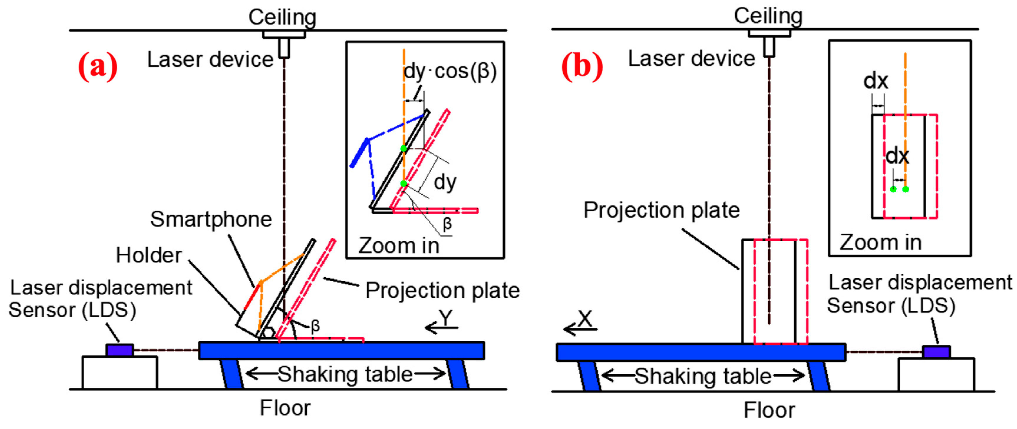
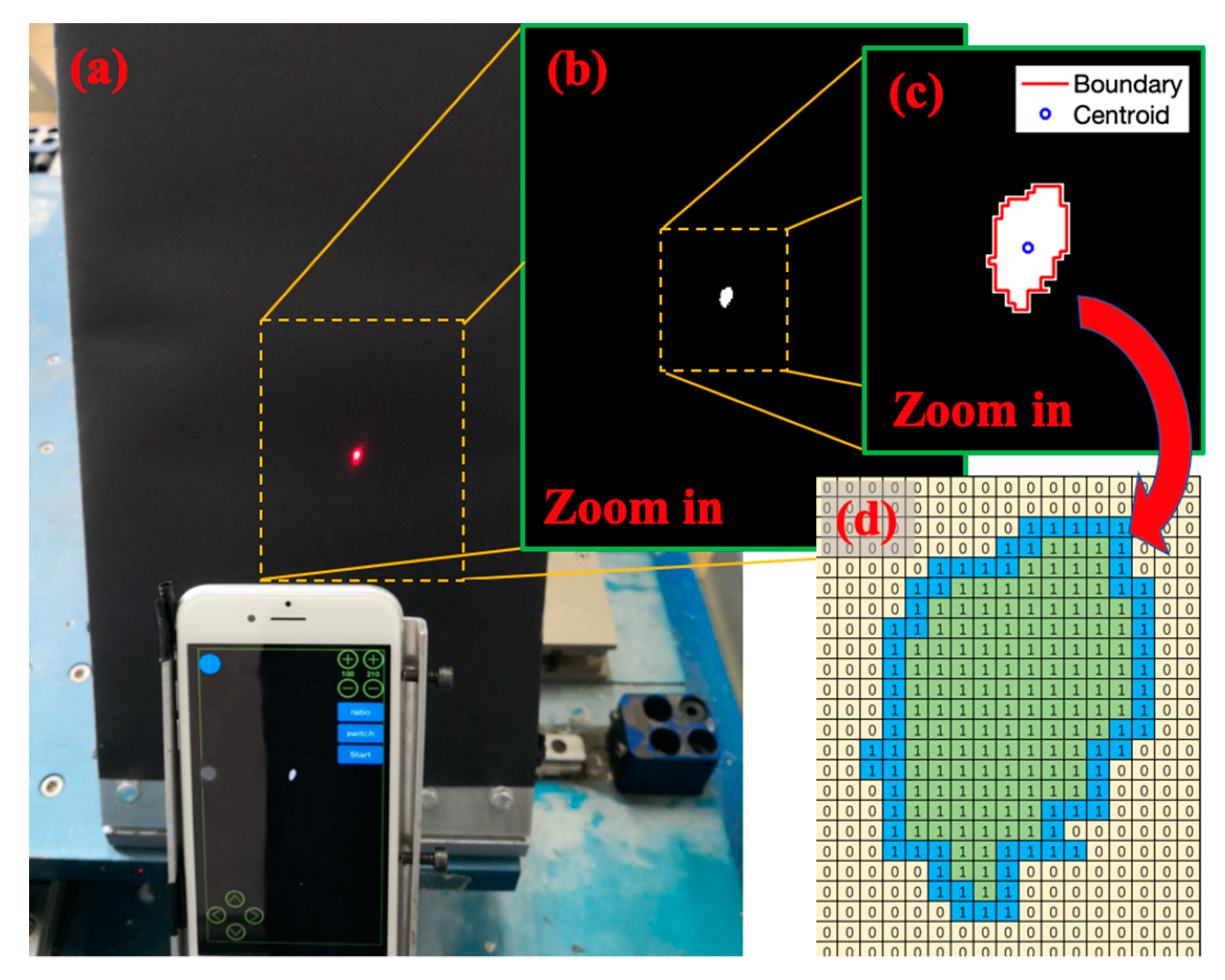
2.1. Image Processing Principle
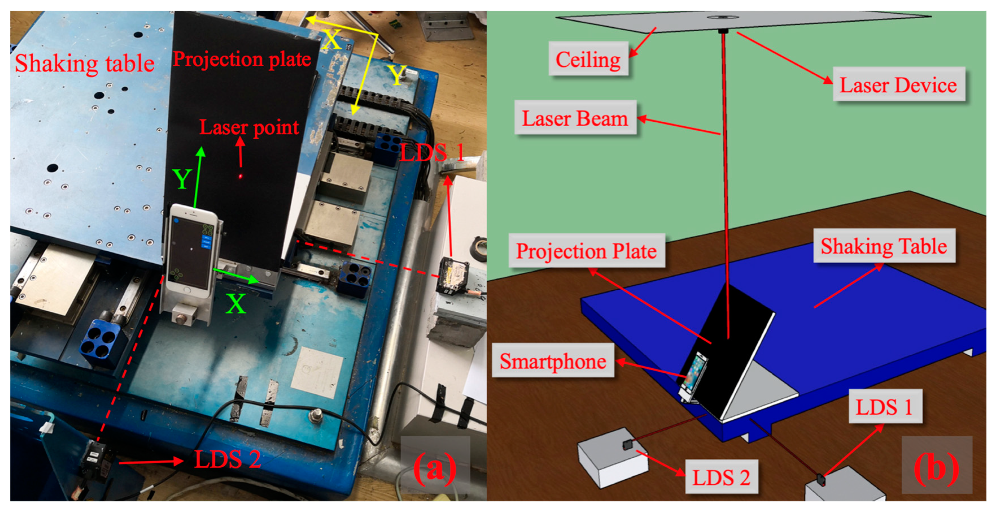
2.2. Experimental Setup
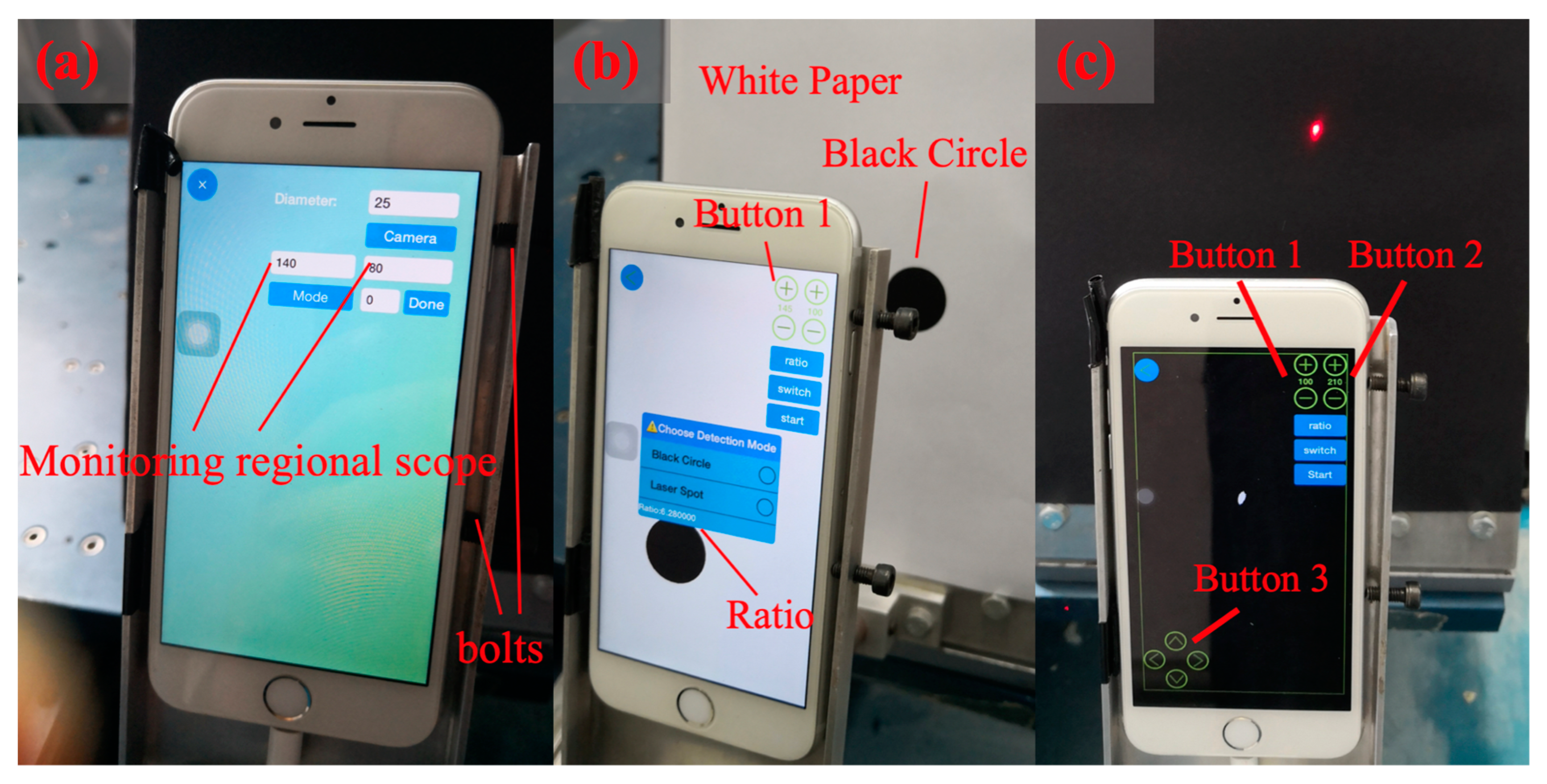
2.3. D-Viewer App Settings
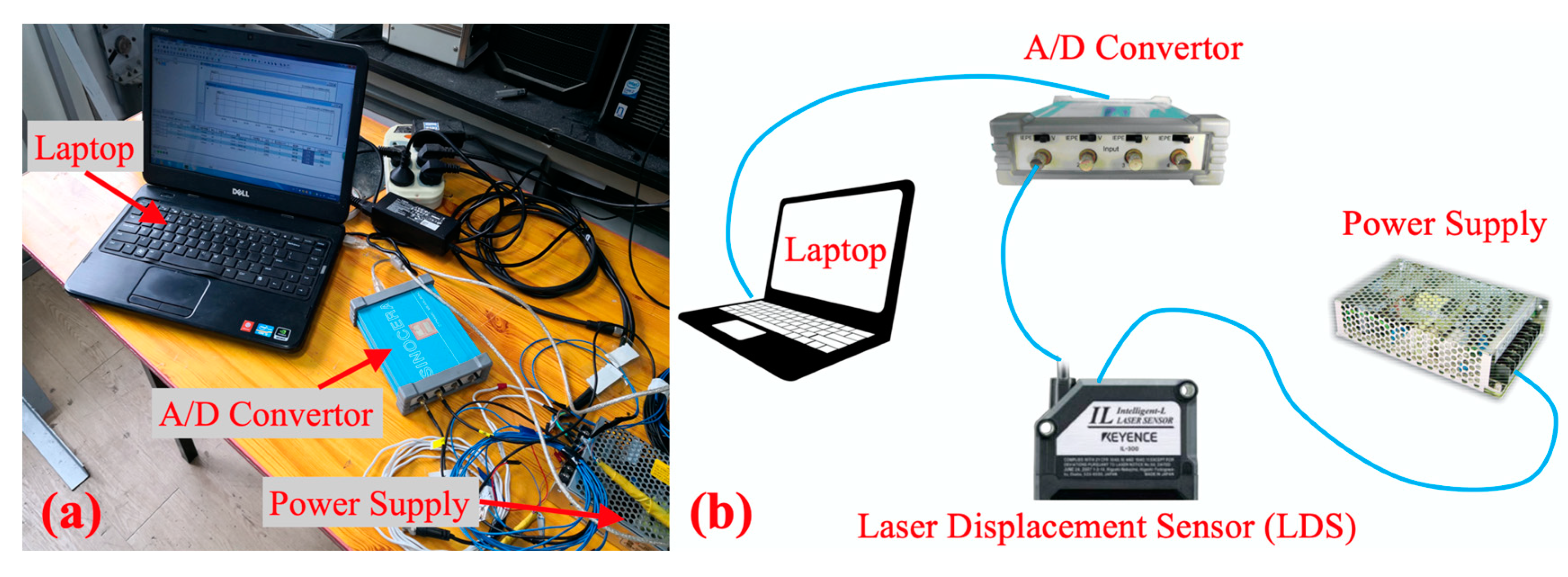
2.4. Reference Sensor
3. Results
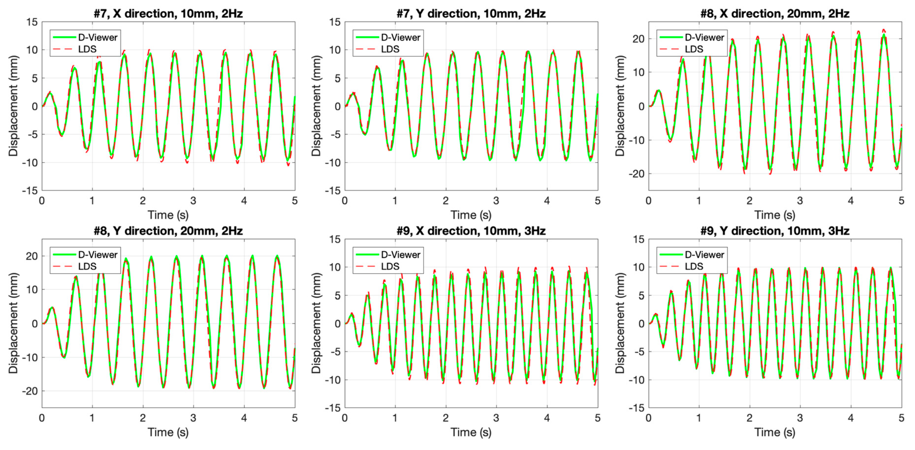
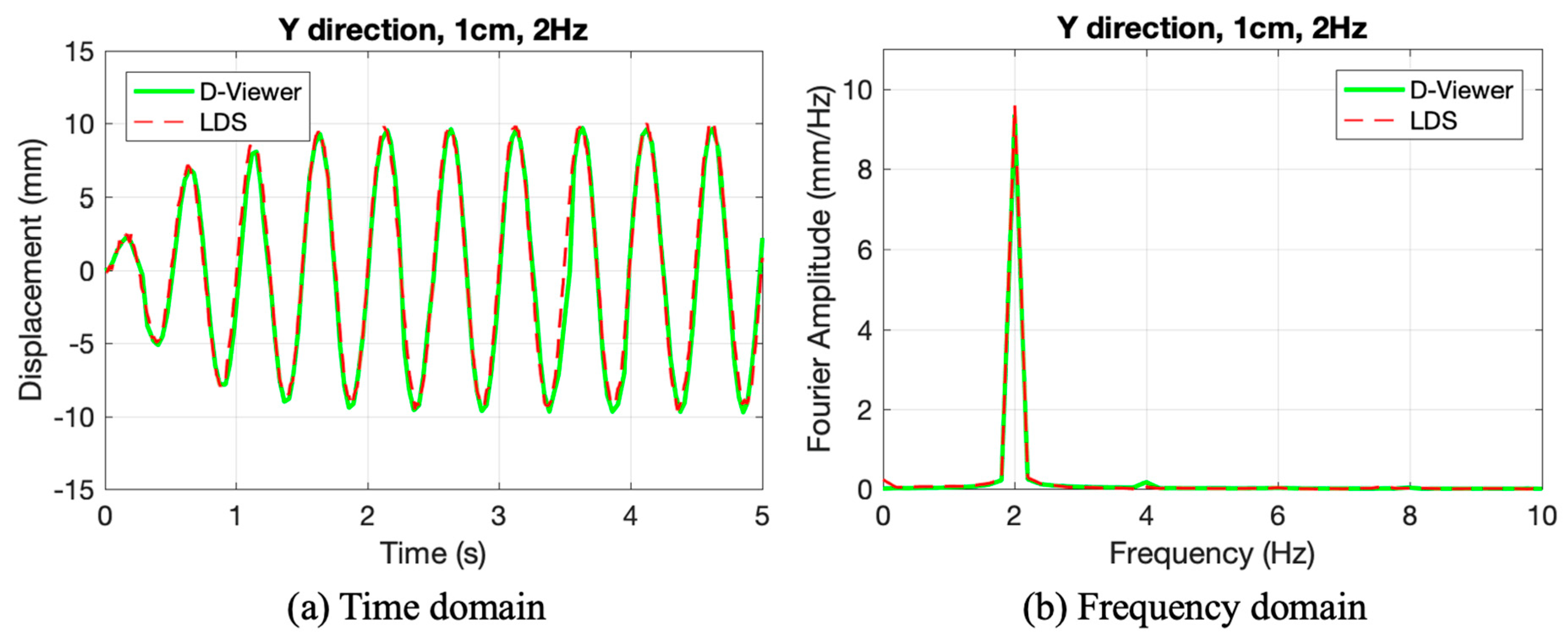
3.1. Sinusoidal Excitation Tests
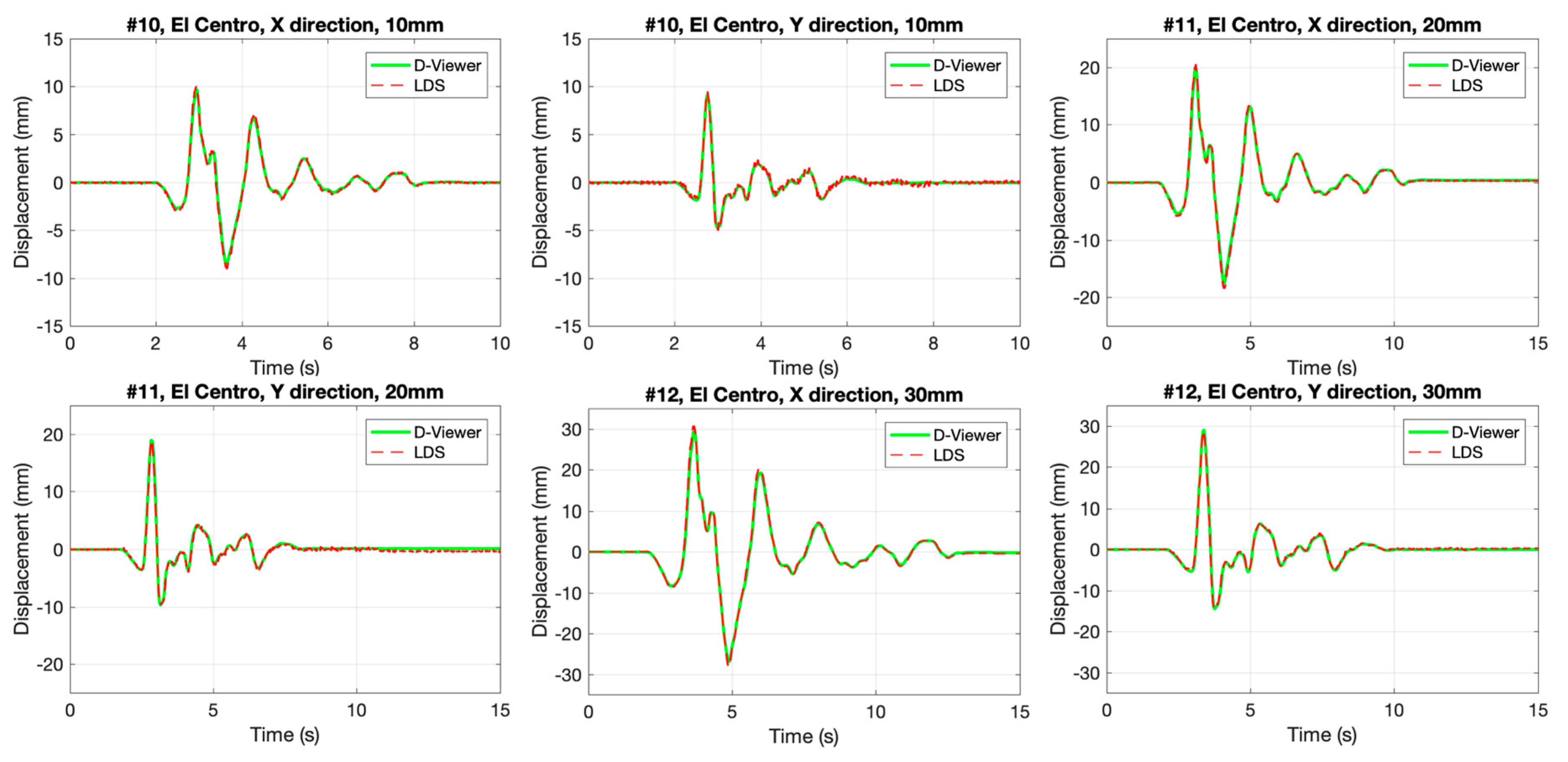
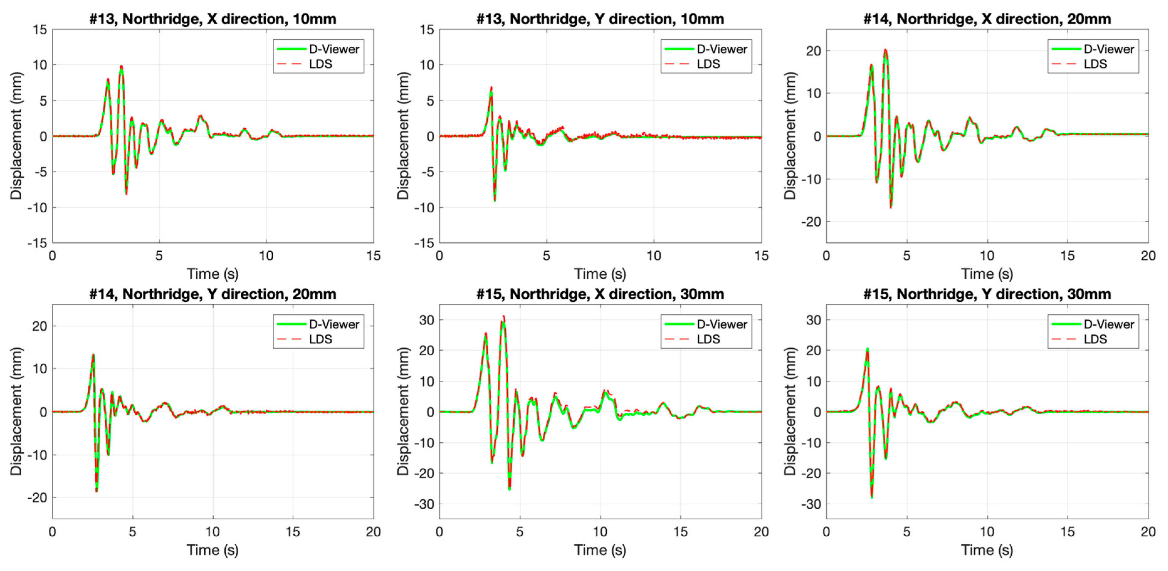
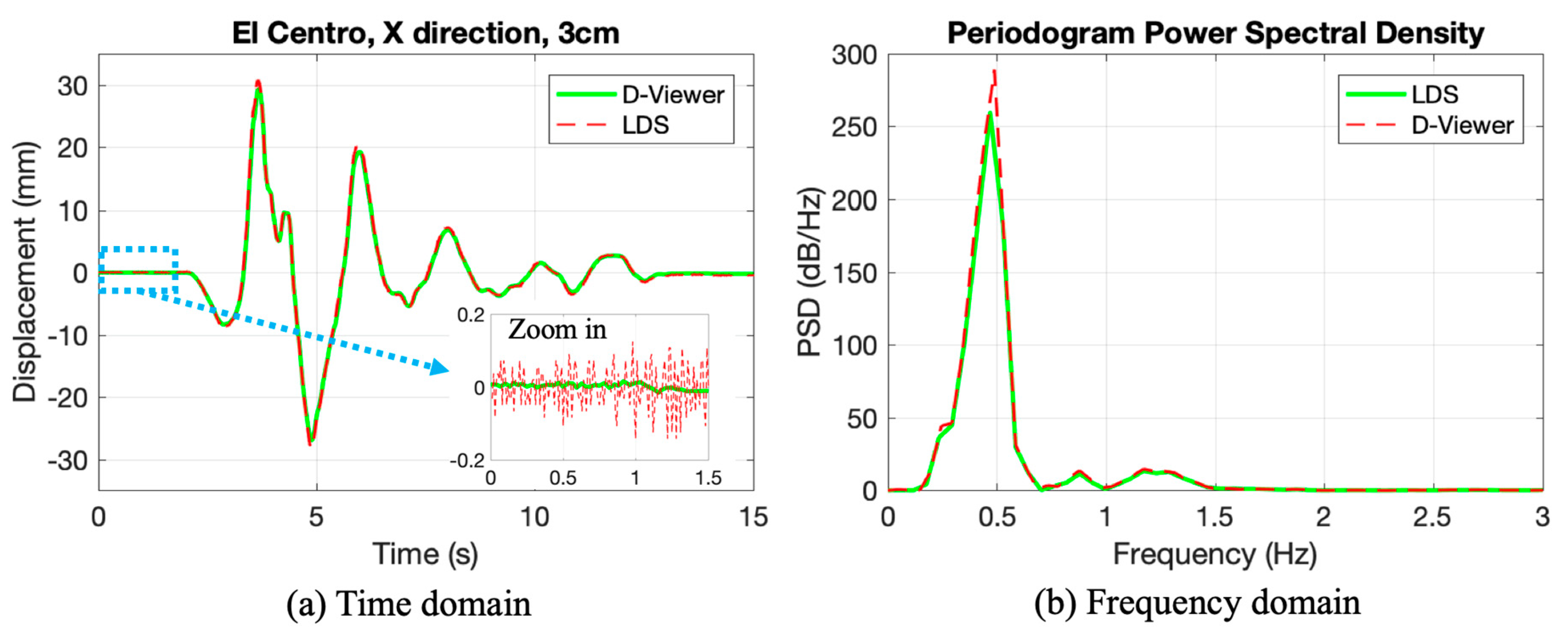
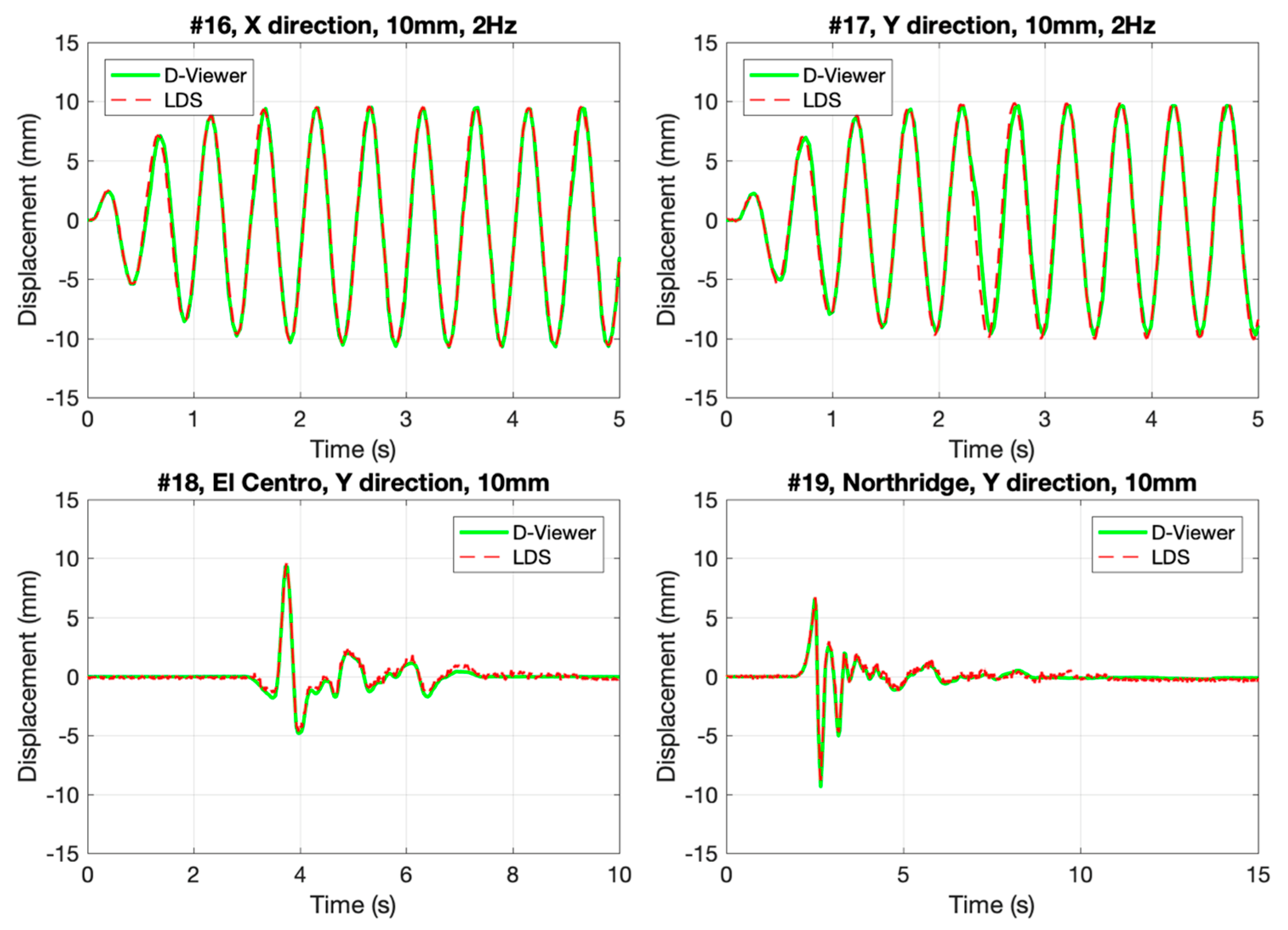
3.2. Seismic Wave Excitation Test
3.3. Night Test
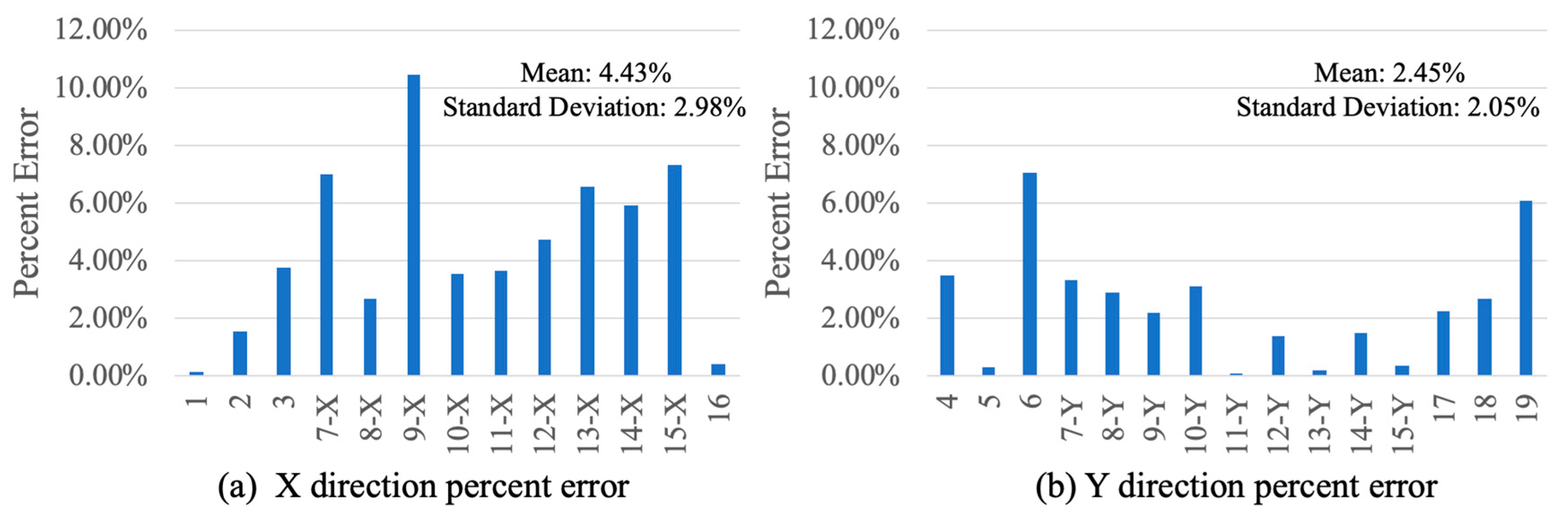
3.4. Error Analysis
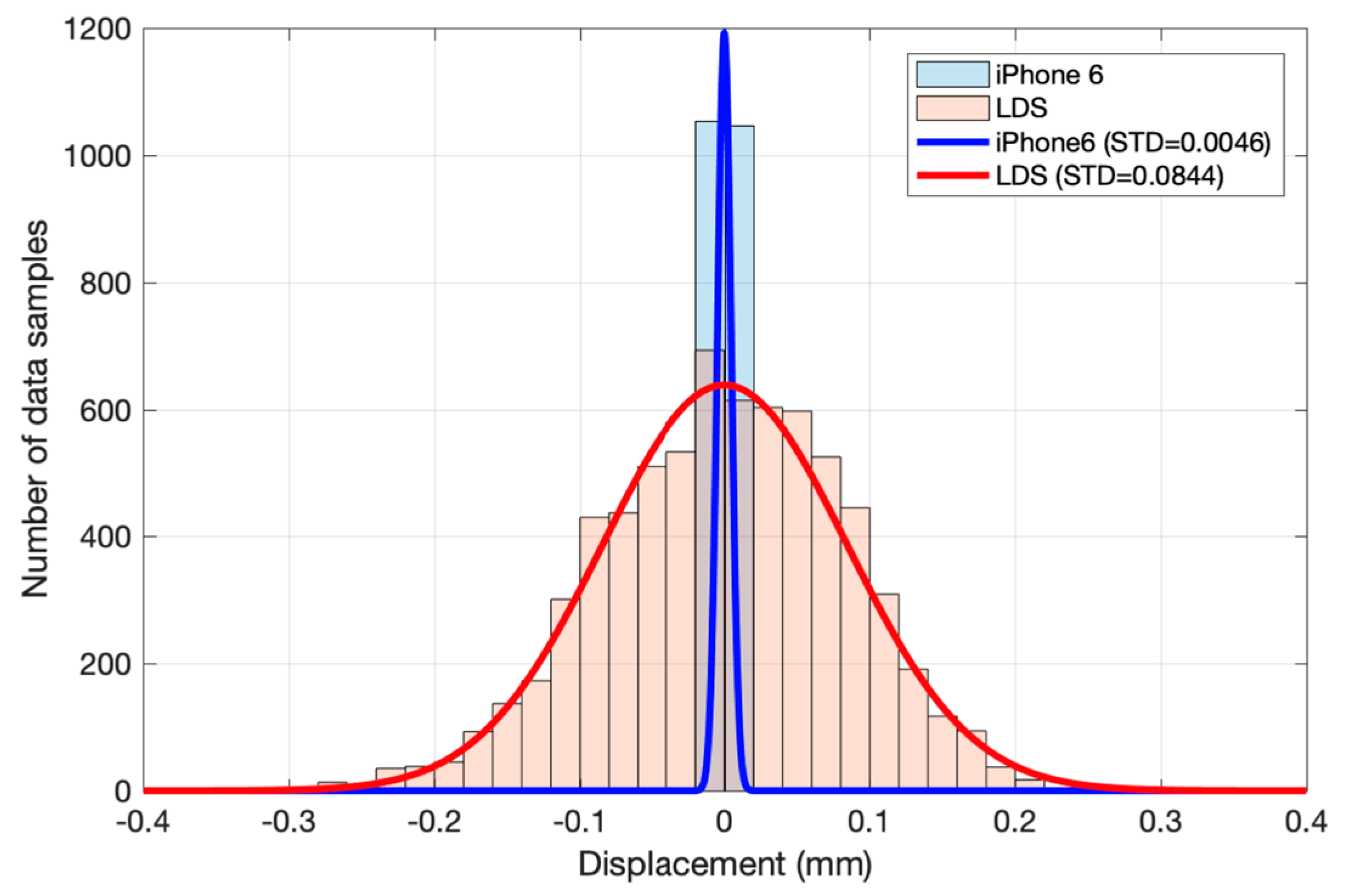
3.5. Sensor Comparison
4. Discussion
- Compared with the LDS, the proposed method performed well in sinusoidal oscillation, seismic wave vibration, and a night test with a real story height 3000 mm. The monitoring results showed that the smartphone coincided with LDS in time history and frequency domain. The good results of the night test show that the image processing method is robust at night so that the method could fulfill continuous measurement.
- From the results of all experiments, the average percent error of the smartphone is 3.37%, with a standard deviation of 2.67%. In the stationary period around 0 mm, the standard deviation is 0.0046 mm, which is much smaller than LDS (0.0844 mm). This means the proposed method has a smaller deviation than LDS. The accuracy of the method is 0.0276 mm. These parameters mean the proposed method is competent in interstory drift monitoring with only marginal error.
- Compared with other similar interstory drift monitoring methods, the method has advantages in terms of precision (accuracy is 0.0276 mm, percent error is 3.37%) and cost, and it has been tested in 19 groups of full-scale experiments. The disadvantage of the method is the low sampling rate of 30 Hz, which needs to be improved in future work.
Author Contributions
Funding
Conflicts of Interest
Appendix A


References
- Pnevmatikos, N.G.; Papavasileiou, G.S.; Konstandakopoulou, F.D.; Papagiannopoulos, G. Influence of rotational component of earthquake excitation to the response of steel slender frame. Mater. Sci. Forum 2019, 968, 294–300. [Google Scholar] [CrossRef]
- FEMA. Multi-Hazard loss estimation methodology-earthquake model technical manual (HAZUS-MH 2.1). Federal Emergency Management Agency, Washington, DC. Available online: https://www.fema.gov/media-library-data/20130726-1820-25045-6286/hzmh2_1_eq_tm.pdf (accessed on 22 March 2020).
- Code for Seismic Design of Buildings (GB 50011-2010). Ministry of Housing and Urban-Rural Development of the People’s Republic of China, Beijing, China. Available online: http://www.mohurd.gov.cn/wjfb/201608/t20160801_228378.html (accessed on 22 March 2020).
- FEMA. Prestandard and Commentary for the Seismic Rehabilitation of Buildings (FEMA 356). Building Seismic Safety Council, Washington, DC. Available online: https://www.fema.gov/media-library-data/20130726-1444-20490-5925/fema_356.pdf (accessed on 22 March 2020).
- Suita, K.; Yamada, S.; Tada, M.; Kasai, K.; Matsuoka, Y.; Shimada, Y. Collapse experiment on 4-story steel moment frame: Part 2 detail of collapse behavior. In Proceedings of the 14th world conference on earthquake engineering, Beijing, China, 12–17 October 2008. [Google Scholar]
- Okazaki, T.; Asce, A.M.; Lignos, D.G.; Asce, A.M.; Hikino, T.; Kajiwara, K. Dynamic Response of a Chevron Concentrically Braced Frame. J. Struct. Eng. 2013, 139, 515–525. [Google Scholar] [CrossRef] [Green Version]
- Zhou, C.; Chase, J.G.; Rodgers, G.W. Degradation evaluation of lateral story stiffness using HLA-based deep learning networks. Adv. Eng. Informatics 2019, 39, 259–268. [Google Scholar] [CrossRef]
- Morfidis, K.; Kostinakis, K. Seismic parameters’ combinations for the optimum prediction of the damage state of R / C buildings using neural networks. Adv. Eng. Softw. 2017, 106, 1–16. [Google Scholar] [CrossRef]
- Hwang, S.-H.; Lignos, D.G. Assessment of structural damage detection methods for steel structures using full-scale experimental data and nonlinear analysis. Bull. Earthq. Eng. 2017, 16, 2971–2999. [Google Scholar] [CrossRef] [Green Version]
- Xiang, P.; Nishitani, A.; Marutani, S.; Kodera, K.; Hatada, T.; Katamura, R.; Kanekawa, K.; Tani, T. Identification of yield drift deformations and evaluation of the degree of damage through the direct sensing of drift displacements. Earthq. Eng. Struct. Dyn. 2016, 45, 2085–2102. [Google Scholar] [CrossRef]
- Skolnik, D.A.; Wallace, J.W. Critical assessment of interstory drift measurements. J. Struct. Eng. 2010, 136, 1574–1584. [Google Scholar] [CrossRef]
- Lemnitzer, A.; Massone, L.M.; Skolnik, D.A.; de la Llera Martin, J.C.; Wallace, J.W. Aftershock response of RC buildings in Santiago, Chile, succeeding the magnitude 8.8 Maule earthquake. Eng. Struct. 2014, 76, 324–338. [Google Scholar] [CrossRef]
- Spina, D.; Lamonaca, B.G.; Nicoletti, M.; Dolce, M. Structural monitoring by the Italian Department of Civil Protection and the case of 2009 Abruzzo seismic sequence. Bull. Earthq. Eng. 2011, 9, 325–346. [Google Scholar] [CrossRef] [Green Version]
- Lotfi, B.; Huang, L. An approach for velocity and position estimation through acceleration measurements. Meas. J. Int. Meas. Confed. 2016, 90, 242–249. [Google Scholar] [CrossRef]
- Dai, F.; Dong, S.; Kamat, V.R.; Lu, M. Photogrammetry assisted measurement of interstory drift for rapid post-disaster building damage reconnaissance. J. Nondestruct. Eval. 2011, 30, 201–212. [Google Scholar] [CrossRef]
- Hou, S.; Zeng, C.; Zhang, H.; Ou, J. Monitoring interstory drift in buildings under seismic loading using MEMS inclinometers. Constr. Build. Mater. 2018, 185, 453–467. [Google Scholar] [CrossRef]
- Li, J.; Xie, B.; Zhao, X. Measuring the interstory drift of buildings by a smartphone using a feature point matching algorithm. Struct. Control Heal. Monit. 2020, 27, e2492. [Google Scholar] [CrossRef]
- Li, H.; Dong, S.; El-Tawil, S.; Kamat, V. Relative Displacement Sensing Techniques for Postevent Structural Damage Assessment: Review. J. Struct. Eng. 2012, 356, 1421–1434. [Google Scholar] [CrossRef]
- Kanekawa, K.; Matsuya, I.; Sato, M.; Tomishi, R.; Takahashi, M.; Miura, S.; Suzuki, Y.; Hatada, T.; Katamura, R.; Nitta, Y.; et al. An experimental study on relative displacement sensing using phototransistor array for building structures. IEEJ Trans. Electr. Electron. Eng. 2010, 5, 251–255. [Google Scholar] [CrossRef]
- Matsuya, I.; Katamura, R.; Sato, M.; Iba, M.; Kondo, H.; Kanekawa, K.; Takahashi, M.; Hatada, T.; Nitta, Y.; Tanii, T.; et al. Measuring relative-story displacement and local inclination angle using multiple position-sensitive detectors. Sensors 2010, 10, 9687–9697. [Google Scholar] [CrossRef] [Green Version]
- Matsuya, I.; Tomishi, R.; Sato, M.; Kanekawa, K.; Nitta, Y.; Takahashi, M.; Miura, S.; Suzuki, Y.; Hatada, T.; Katamura, R.; et al. Development of lateral displacement sensor for real-time detection of structural damage. IEEJ Trans. Electr. Electron. Eng. 2011, 6, 266–272. [Google Scholar] [CrossRef]
- Islam, M.N.; Zareie, S.; Alam, M.S.; Asce, M.; Seethaler, R.J. Novel Method for Interstory Drift Measurement of Building Frames Using Laser-Displacement Sensors. J.Struct. Eng. 2016, 142, 4–7. [Google Scholar] [CrossRef]
- McCallen, D.; Petrone, F.; Coates, J.; Repanich, N. A laser-based optical sensor for broad-band measurements of building earthquake drift. Earthq. Spectra 2017, 33, 1573–1598. [Google Scholar] [CrossRef] [Green Version]
- Ozer, E.; Feng, M.Q.; Feng, D. Citizen sensors for SHM: Towards a crowdsourcing platform. Sensors 2015, 15, 14591–14614. [Google Scholar] [CrossRef]
- Zhao, X.; Liu, H.; Yu, Y.; Zhu, Q.; Hu, W.; Li, M.; Ou, J. Displacement monitoring technique using a smartphone based on the laser projection-sensing method. Sensors Actuators A Phys. 2016, 246, 35–47. [Google Scholar] [CrossRef]
- Xie, B.; Li, J.; Zhao, X. Research on damage detection of a 3D steel frame model using smartphones. Sensors 2019, 19, 745. [Google Scholar] [CrossRef] [PubMed] [Green Version]
- Wang, N.; Ri, K.; Liu, H.; Zhao, X. Structural Displacement Monitoring using Smartphone Camera and Digital Image Correlation. IEEE Sens. J. 2018, 18, 4664–4672. [Google Scholar] [CrossRef]
- Kong, Q.; Allen, R.M.; Kohler, M.D.; Heaton, T.H.; Bunn, J. Structural Health Monitoring of Buildings Using Smartphone Sensors. Seismol. Res. Lett. 2018, 89, 594–602. [Google Scholar] [CrossRef]
- Shrestha, A.; Dang, J.; Wang, X. Development of a smart-device-based vibration-measurement system: Effectiveness examination and application cases to existing structure. Struct. Control Heal. Monit. 2018, 25, e2120. [Google Scholar] [CrossRef]
- Shrestha, A.; Ph, D.; Dang, J.; Asce, A.M.; Wang, X.; Matsunaga, S. Smartphone-Based Bridge Seismic Monitoring System and Long-Term Field Application Tests. J. Struct. Eng. 2020, 146, 1–14. [Google Scholar] [CrossRef]
- Gonzalez, R.C.; Woods, R.E. Digital Image Processing, 3rd ed.; Prentice-Hall: New York, NY, USA, 2007. [Google Scholar]
- Manolakis, D.G.; Ingle, V.K. Applied Digital Signal Processing: Theory and Practice; Cambridge University Press: New York, NY, USA, 2011. [Google Scholar]
- Xu, Y.; Brownjohn, J.M.W. Vision-based systems for structural deformation measurement: Case studies. Proc. Inst. Civ. Eng. Struct. Build. 2018, 171, 1–14. [Google Scholar] [CrossRef] [Green Version]
- Luo, L.; Feng, M.Q. Edge-Enhanced Matching for Gradient-Based Computer Vision Displacement Measurement. Comput. Civ. Infrastruct. Eng. 2018, 33, 1019–1040. [Google Scholar] [CrossRef]
- Xu, Y.; Brownjohn, J.; Kong, D. A non-contact vision-based system for multipoint displacement monitoring in a cable-stayed footbridge. Struct. Control Heal. Monit. 2018, 25, 1–23. [Google Scholar] [CrossRef] [Green Version]
- Xiong, C.; Lu, X.; Lin, X.; Xu, Z.; Ye, L. Parameter Determination and Damage Assessment for THA-Based Regional Seismic Damage Prediction of Multi-Story Buildings. J. Earthq. Eng. 2017, 21, 461–485. [Google Scholar] [CrossRef]


| Instruments | LDS | A/D Converter | Power Supply | Laptop |
|---|---|---|---|---|
| Maker | Keyence | Sinocera Piezotronics Inc. | Mean Well | Dell |
| Model | IL-300 | YE6231 | NES-100-12 | Inspiron 3420 |
| Supplement | Measurement range: 160–450 mm | Signal to noise ratio: 80 dB; 4 channels | Output voltage: 12 V; Direct current | CPU: i5-3210M; RAM: 4G; System: Window 7 |
| Test Number | Direction | Amplitude (mm) | Frequency (Hz) |
|---|---|---|---|
| #1 | X | 10 | 2 |
| # 2 | X | 20 | 2 |
| # 3 | X | 10 | 3 |
| # 4 | Y | 10 | 2 |
| # 5 | Y | 20 | 2 |
| # 6 | Y | 10 | 3 |
| # 7 | X, Y | 10 | 2 |
| # 8 | X, Y | 20 | 2 |
| # 9 | X, Y | 10 | 3 |
| Test Number | Seismic Wave | Direction | Amplitude (mm) |
|---|---|---|---|
| #10 | El Centro | X, Y | 10 |
| #11 | El Centro | X, Y | 20 |
| #12 | El Centro | X, Y | 30 |
| #13 | Northridge | X, Y | 10 |
| #14 | Northridge | X, Y | 20 |
| #15 | Northridge | X, Y | 30 |
| Test Number | Waveform | Direction | Amplitude (mm) |
|---|---|---|---|
| #16 | Sinusoidal wave | X | 10 |
| #17 | Sinusoidal wave | Y | 10 |
| #18 | El Centro | Y | 10 |
| #19 | Northridge | Y | 10 |
| Method | Precision (mm) | Percent Error (%) | Story Height (mm) | Measurement Range (mm) | Maximum Sampling Rate (Hz) |
|---|---|---|---|---|---|
| Dai [15] | -- 1 | 9.44 2 | -- | -- | Static measurement |
| Hou [16] | -- | 7.60 | 1600 | -- | -- |
| Li [17] | 0.1664 | 3.09 | 3000 | 30 | |
| Kanekawa [19] | 0.1100 | -- | 8900 | 200 | |
| Matsuya [20] | 0.1500 | -- | 3500 | -- | |
| Matsuya [21] | 0.0600 | -- | 3500 | 1000 | |
| Islam [22] | -- | 10.16 2 | 200 | -- | -- |
| McCallen [23] | 1.0000 | -- | 3000 | 384 | |
| This study | 0.0276 | 3.37 | 3000 | 30 |
© 2020 by the authors. Licensee MDPI, Basel, Switzerland. This article is an open access article distributed under the terms and conditions of the Creative Commons Attribution (CC BY) license (http://creativecommons.org/licenses/by/4.0/).
Share and Cite
Li, J.; Xie, B.; Zhao, X. A Method of Interstory Drift Monitoring Using a Smartphone and a Laser Device. Sensors 2020, 20, 1777. https://doi.org/10.3390/s20061777
Li J, Xie B, Zhao X. A Method of Interstory Drift Monitoring Using a Smartphone and a Laser Device. Sensors. 2020; 20(6):1777. https://doi.org/10.3390/s20061777
Chicago/Turabian StyleLi, Jinke, Botao Xie, and Xuefeng Zhao. 2020. "A Method of Interstory Drift Monitoring Using a Smartphone and a Laser Device" Sensors 20, no. 6: 1777. https://doi.org/10.3390/s20061777
APA StyleLi, J., Xie, B., & Zhao, X. (2020). A Method of Interstory Drift Monitoring Using a Smartphone and a Laser Device. Sensors, 20(6), 1777. https://doi.org/10.3390/s20061777