Article

Optimizing an Adaptive Neuro-Fuzzy Inference System for Spatial Prediction of Landslide Susceptibility Using Four State-of-the-art Metaheuristic Techniques

1
Department of Civil Engineering, Kermanshah University of Technology, 6715685420 Kermanshah, Iran
2
The Centre for Advanced Modelling and Geospatial Information Systems (CAMGIS), Faculty of Engineering and Information Technology, University of Technology, Sydney, NSW 2007, Australia
3
Department of Energy and Mineral Resources Engineering, Sejong University, Choongmu-gwan, 209 Neungdong-ro Gwangjin-gu, Seoul 05006, Korea
4
Informetrics Research Group, Ton Duc Thang University, Ho Chi Minh City, Vietnam
5
Faculty of Civil Engineering, Ton Duc Thang University, Ho Chi Minh City, Vietnam
6
Department of Geology & Geophysics, College of Science, King Saud Univ., P.O. Box 2455, Riyadh 11451, Saudi Arabia
*
Author to whom correspondence should be addressed.
Sensors 2020, 20(6), 1723; https://doi.org/10.3390/s20061723
Submission received: 25 February 2020 / Revised: 9 March 2020 / Accepted: 17 March 2020 / Published: 19 March 2020

Abstract

:
Four state-of-the-art metaheuristic algorithms including the genetic algorithm (GA), particle swarm optimization (PSO), differential evolutionary (DE), and ant colony optimization (ACO) are applied to an adaptive neuro-fuzzy inference system (ANFIS) for spatial prediction of landslide susceptibility in Qazvin Province (Iran). To this end, the landslide inventory map, composed of 199 identified landslides, is divided into training and testing landslides with a 70:30 ratio. To create the spatial database, thirteen landslide conditioning factors are considered within the geographic information system (GIS). Notably, the spatial interaction between the landslides and mentioned conditioning factors is analyzed by means of frequency ratio (FR) theory. After the optimization process, it was shown that the DE-based model reaches the best response more quickly than other ensembles. The landslide susceptibility maps were developed, and the accuracy of the models was evaluated by a ranking system, based on the calculated area under the receiving operating characteristic curve (AUROC), mean absolute error, and mean square error (MSE) accuracy indices. According to the results, the GA-ANFIS with a total ranking score (TRS) = 24 presented the most accurate prediction, followed by PSO-ANFIS (TRS = 17), DE-ANFIS (TRS = 13), and ACO-ANFIS (TRS = 6). Due to the excellent results of this research, the developed landslide susceptibility maps can be applied for future planning and decision making of the related area.

Graphical Abstract

1. Introduction

Slope failures are ubiquitous major disasters causing many financial and physical damages worldwide every year. Varnes and Radbruch-Hall [1] presented a definition of a landslide as any downward mass movement caused by gravity on slopes (e.g., artificial deposits, soil, and natural cliffs). Global reports state that developing countries have witnessed the majority (more than 90%) of the landslide events that have occurred around the world. Additionally, landslides are responsible for more than 17% of the reported fatalities [2]. Due to the large number of landslides that have occurred in recent decades, Iran is recognized as a landslide-prone area. It is noteworthy that the largest debris flow in the world, the Seimareh landslide, occurred in western Iran [3]. In another event, slope cutting and removal of the toe buttress triggered the Manjil landslide in 2013. It occurred on the Qazvin–Rasht freeway and led to blockage of the freeway [4].
As is known, landslide susceptibility mapping is an essential prerequisite for landslide risk management [5,6]. A proper landslide risk assessment entails determining the effective landslide parameters for discovering the spatial relationship between them and occurred landslides. Up to now, plenty of theories have been utilized for this purpose in many specific areas. Some of them are based on statistical rules, which aim to determine the importance of each independent landslide factor through assigning weights. Novel intelligent models are also proposed for approximating the susceptibility of an area through learning the mathematical relationship between a landslide and its related factors [7,8].
Many scholars have employed statistical-based methods for landslide susceptibility assessment [9,10,11]. Fayez, et al. [12] successfully implemented the FR model for landslide susceptibility assessment in India. In a comparative study, Chen, et al. [13] used frequency ratio (FR), weights-of-evidence (WoE), and statistical index (SI) methods for producing the landslide susceptibility map of Qianyang County (China). Considering 13 landslide-related factors, they achieved the proposed maps with 78.53%, 79.35%, and 79.40% prediction accuracies, respectively for WoE, SI, and FR models. Analytical hierarchy process (AHP) is another popular method employed in landslide susceptibility mapping [14,15]. Yan, et al. [16] used the integration of AHP with normalized FR with the cloud model for landslide susceptibility assessment. Moreover, Yang, et al. [17] investigated the landslide susceptibility modelling in Sichuan Province (China) using a spatial logistic regression (SLR) approach. They also developed a GeoDetector-based method for the proper selection of the landslide-conditioning parameters. Their findings showed that the estimation precision of the proposed model was about 11.9% higher than typical logistic regression (LR). Liu and Duan [18] conducted a comparison among the WoE, SI, and Index of Entropy (IoE) for quantitative assessment of landslide susceptibility in Shangnan County (China). According to the results, the WoE (with around 76 and 75% accuracy rate for the training and testing data, respectively) outperformed two other models. A new integrated statistical method, called B-GeoSVC, was proposed by Yang, et al. [19] as a reliable evaluative approach for both regional and local scales.
Moreover, various intelligent predictive models like the artificial neural network (ANN), adaptive neuro-fuzzy inference system (ANFIS), and support vector machine (SVM) have been promisingly employed for forecasting the landslide susceptibility risk [20,21,22]. Aditian, et al. [23] showed the superiority of the ANN (success rate = 0.734) for landslide susceptibility evaluation in Indonesia, in comparison with FR (success rate = 0.688), and LR (success rate = 0.687). Polykretis, et al. [24] examined the capability of different models of ANFIS. Based on the calculated prediction accuracies (i.e., between 0.7 to 0.90), all implemented models are reliable enough to be used for the mentioned purpose. Likewise, Chen, et al. [25] evaluated the capability of three state-of-the-art predictive models of ANFIS combined with FR (ANFIS-FR), generalized additive model (GAM), and SVM in landslide susceptibility assessment in Hanyuan County (China). This study showed that SVM presents the most accurate prediction (accuracy = 87.5%), followed by ANFIS-Fr (accuracy = 85.1%) and GAM (accuracy = 84.6%). Pham, et al. [26] proposed a hybrid predictive model named rotation forest-based radial basis function neural network for landslide susceptibility zonation of the Himalayan area, India. They found that the proposed model could be a good alternative for this aim, due to the better performance than LR, multi-layer perceptron neural network, the hybrid of rotation forest and decision trees (RFDT), and naïve Bayes (NB).
Furthermore, many studies have focused on the development of hybrid metaheuristic algorithms incorporated with typical models in order to achieve more powerful predictive tools [27,28,29]. Nguyen, et al. [30] used particle swarm optimization (PSO) and artificial bee colony (ABC) metaheuristic techniques to optimize the performance of the ANN for landslide susceptibility mapping at northern Iran. The calculated area under the curve (AUC) values revealed that the prediction accuracy of the MLP increased from nearly 77% to around 86% and 80%, respectively by applying the PSO and ABC algorithms. Likewise, Chen, et al. [31] coupled three optimization techniques of PSO, genetic algorithm (GA), and differential evolution (DE) with the ANFIS for spatial hazard assessment of landslide in Hanyuan County (China). The AUC of all three ensembles obtained higher than 0.75. In addition, the ANFIS-DE (AUC = 0.844) emerged as the most promising ensemble technique, followed by ANFIS-GA (AUC = 0.821), and ANFIS-PSO (AUC = 0.780). Tien Bui, et al. [32] combined imperialist competitive algorithm (ICA) and relevance vector machine (RVM) for landslide susceptibility modelling of Lang Son City (Vietnam). At the same time, they considered the SVM and LR as benchmark models. They showed that the suggested RVM-ICA outperformed SVM and LR with respective AUCs of 0.92, 0.91, and 0.87, respectively.
As mentioned above, various studies have successfully used the ANFIS for landslide susceptibility assessment [33,34]. However, hybrid ensembles of this model have been broadly used for similar applications like flood [35] and forest fire susceptibility [36] assessment. To the best knowledge of the authors, optimizing this model with metaheuristic algorithms for landslide susceptibility mapping has been rarely explored [37]. Hence, the essential novelty of this research lies in synthesizing four wise evolutionary algorithms, namely GA, PSO, DE, and ant colony optimization (ACO) with ANFIS to remedy its computational shortcomings like local minimum [38] and dimension dangers [31] in spatial modelling of the landslide. Besides, the study area (i.e., Qazvin County, Iran) is a relatively landslide-prone area that has not been sufficiently investigated in prior studies. In this regard, followed by providing the required spatial database, the FR index is calculated to measure the importance of each sub-class of the considered conditioning factors. Then, the landslide susceptibility maps are generated by each model, and the results are validated by the area under the receiving operating characteristic curve (AUROC), mean square error (MSE), and mean absolute error (MAE) accuracy criteria. The proposed models, however, may be applicable to other areas with similar environmental conditions.

2. Materials and Methods
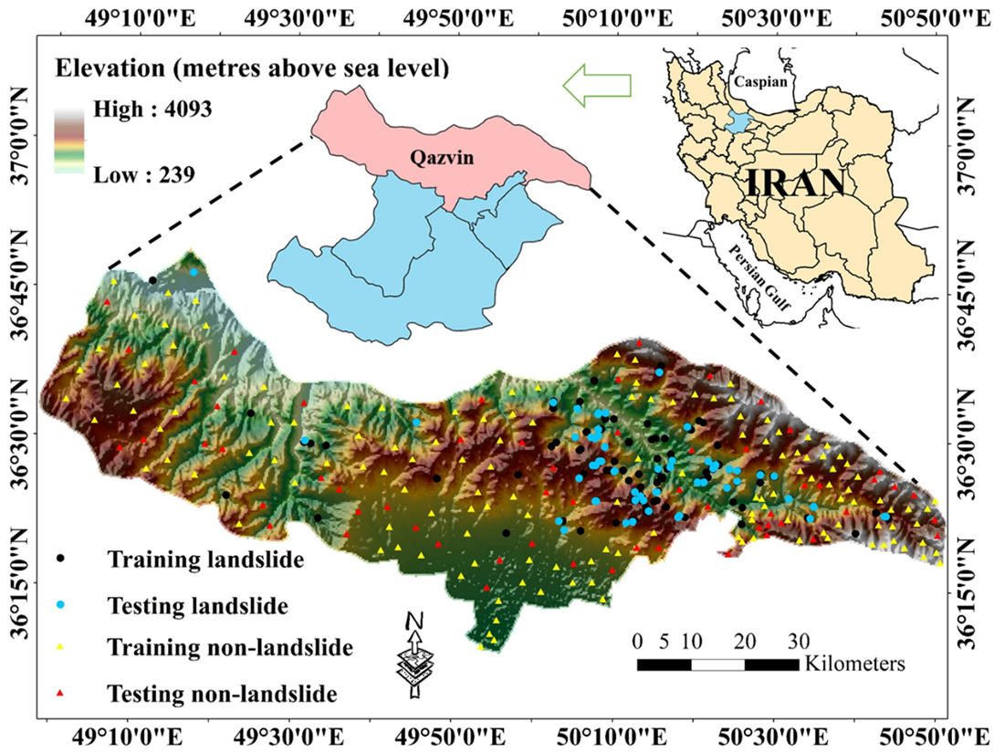
2.1. Study Area

The study area is Qazvin County, located in Qazvin Province, one of the 31 provinces of Iran, in the north-western part of the country. Figure 1 illustrates the exact location of Qazvin County. It covers roughly 4992 km2 and lies within the longitude 48°58′ to 50°51′ E and latitude 36°08′ to 36°48′ N. In the northern watersheds of Qazvin, the Shahrood river flows, which is the result of joining Taleghan and Alamut rivers [39]. Due to the presence of the Alborz mountains, this area is known to have a mountainous climate [40], and approximately half of the area is covered by mountainous pastures. The altitude ranges from 239 to 4093 m above the sea level, and it is higher than 1200 m in the major part of the area [4]. The average temperature of the hot and cold seasons is reported as approximately 28 °C and 1 °C, respectively. Also, the annual precipitation in most parts of the county is higher than 500.5 mm [40]. The slope ranges from 0° to 45°, where more than 70% of the area contains gentle slopes (i.e., slope lower than 15°). According to the Geology Survey of Iran (GSI), Qazvin County lies on a bed with 25 geology units. Among them, two groups of Dacitic andesitic volcanic tuff and sandy limestone, Marl, calcareous sandstone, and minor conglomerate are the most common rocks, covering 19.45% and 16.20% of the county, respectively. Also, the soil map shows that approximately 60% of the study area is categorized as Rock Outcrops/Entisols soil.
The spatial distribution of the identified landslide, as well as the non-landslide points, is illustrated in Figure 1 over the hill shade map of the study area. According to this figure, the majority of slope failures have occurred in the right half of the Qazvin County, mostly along the territorial roads and detected faults.

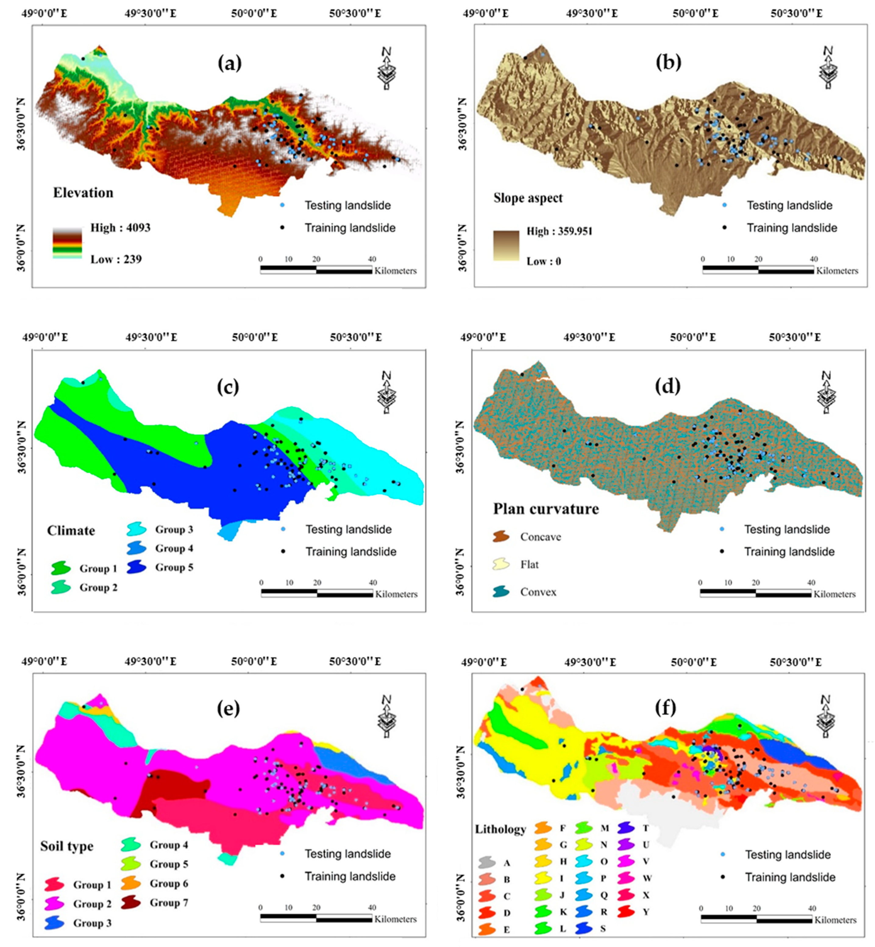
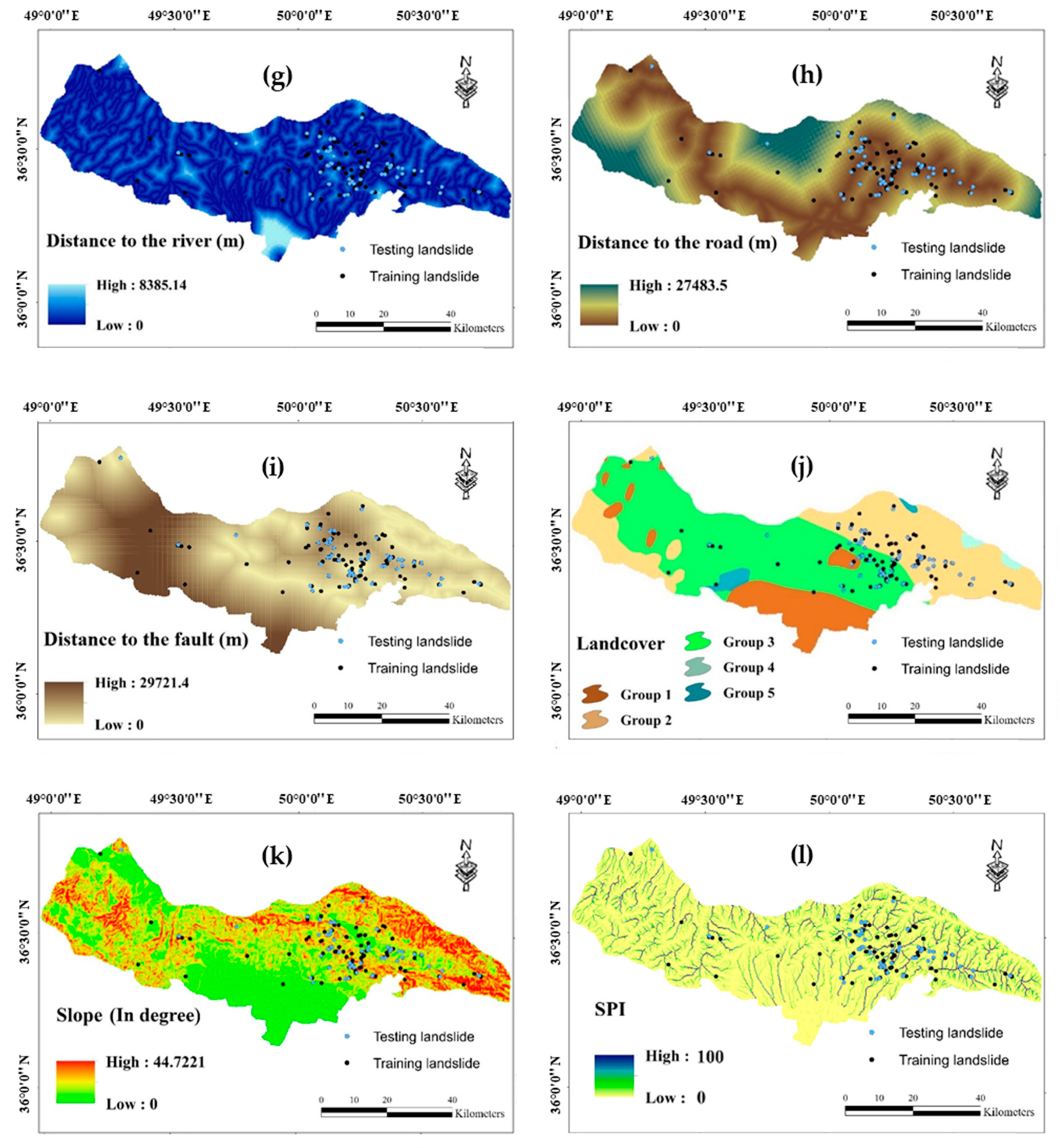
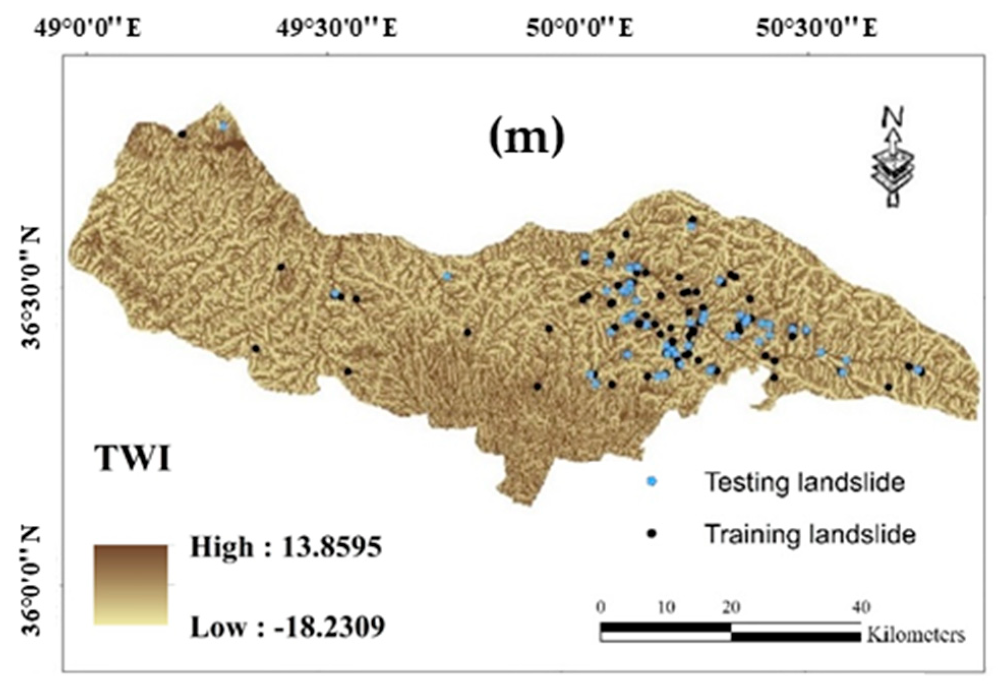
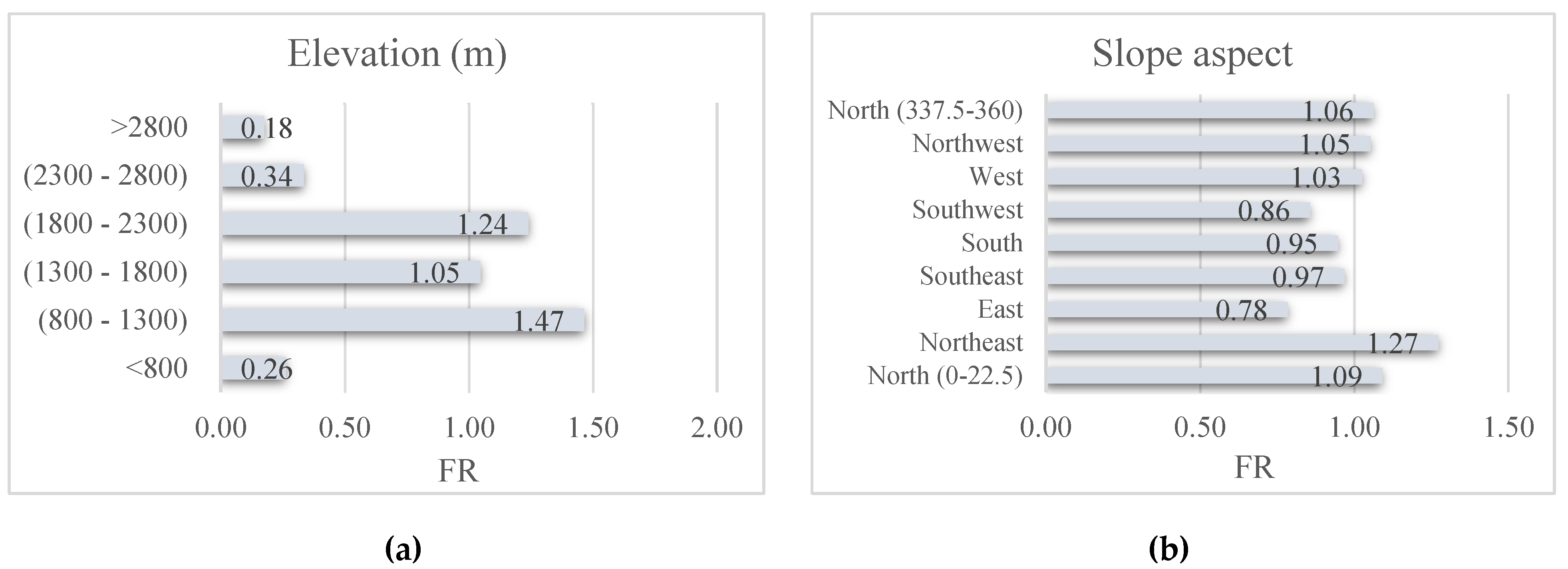
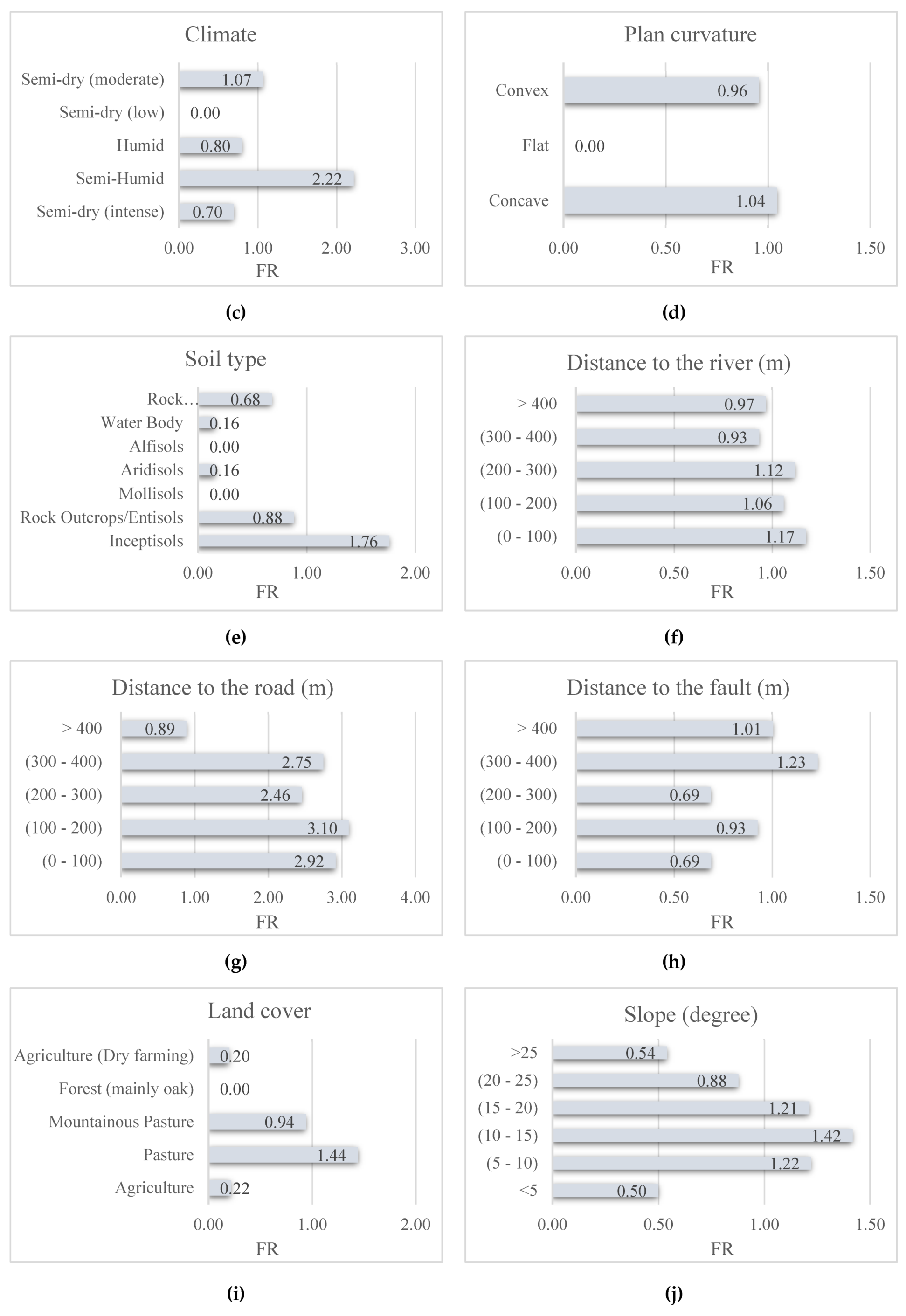
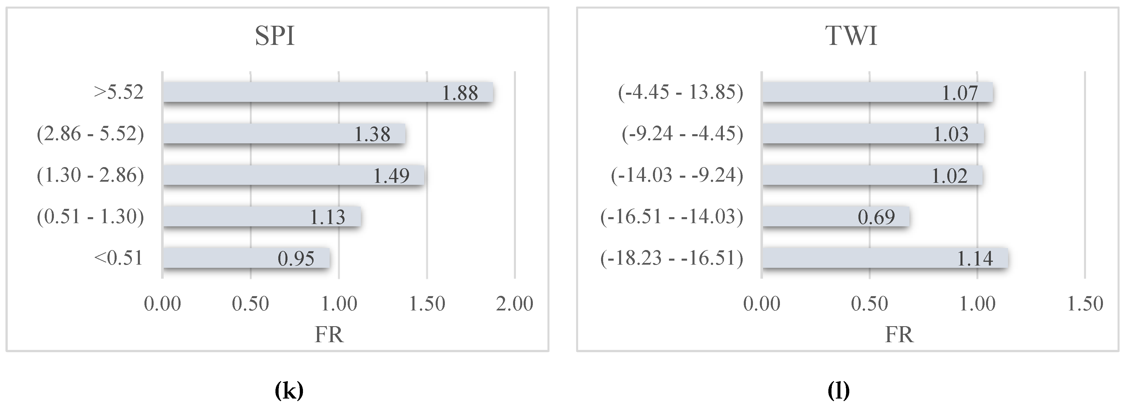
2.2. Data Preparation and Spatial Relation Between the Landslide and Related Factors
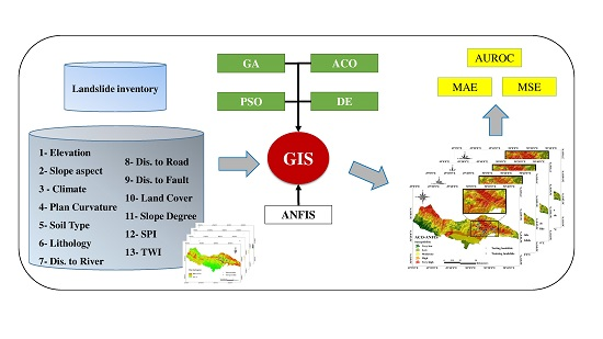
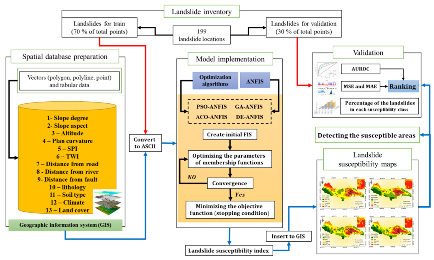
When it comes to implementing intelligent models, using a valid dataset is very important [41]. The dataset used in this study consists of thirteen landslide condition factors, including elevation, slope aspect, climate, plan curvature, soil type, lithology, distance to the river, distance to the road, distance to the fault, land cover, slope degree, stream power index (SPI), and topographic wetness index (TWI) as the input variables, and landslide occurrence (0 = no landslide and 1 = landslide) as the target variable. All layers are produced and processed in the geographic information system (GIS) with a pixel size of 10 × 10 m [42,43,44]. Figure 2 illustrates a map of the mentioned landslide-related factors.
Providing a valid landslide inventory map is an essential step in the susceptibility analysis of this natural hazard [45]. In the study area, a total of 199 landslides were marked using previous records from the national geoscience database of Iran (NGDIR), as well as satellite imagery (IRS: LISS-III) and interpreting the aerial photos (in 1:25000 scale) covering the past 20 years (i.e., 1995–2015) [46]. It should be noted that the identified landslides are mostly translational and rotational slope failures are rarely observed. Some field photographs of landslides that occurred in Qazvin Province can be found in a research by Arjmandzadeh, et al. [47]. Out of the marked landslides, 139 events (i.e., 70% of the whole dataset) are randomly selected and used for the training phase, and the remaining 60 events (i.e., 30% of the whole dataset) are allocated to the validation phase. Besides, 199 non-landslide points are randomly produced over the areas devoid of landslides and divided into the training and testing parts with the same proportions.
The FR theory is also considered to measure the spatial correlation between the landslides and conditioning factors. Each sub-class of the landslide conditioning layers receives an FR value. In this sense, the higher the values of FR, the more significant of the proposed sub-class [48]. This index is expressed as follows:
F R = N l a n d s l i d e N d o m a i n
where Nlandslide and Ndomain respectively denote the percentage of the landslide events located in the proposed sub-class and the percentage of the domain covered by it. Figure 3 shows the results of the FR analysis.
A digital elevation model (DEM) of the Qazvin County with 10 m spatial resolution was created from topographic data (contours and survey base points) at 1:25000 scale. This layer is subsequently used for generating the GIS layer of some landslide conditioning factors including elevation, plan curvature, slope aspect, and slope degree of the study area. The altitude varies in the range of 239−4093 m, and more than 70% of the area is above 700 m. The elevation layer was classified into six classes with 500 m intervals [49] and the highest FR is obtained for the elevations between 800 and 1300. Based on the values in the range of [0–360°], the slope aspect layer is classified into nine groups including North (0–22.5°), North-East (22.5–67.5°), East (67.5–112.5°), South-East (112.5–157.5°), South (157.5–202.5°), South-West (202.5–247.5°), West (247.5–292.5°), North-West (292.5–337.5°) and North (337.5–360°). The FR analysis shows that North (0–22.5°), North-East, North-West, West, and North (337.5–360°) have this value larger than 1. Plan curvature was classified into three categories of Concave (<−0.001), Flat (−0.001–0.001), and Convex (>0.001) [50], which the first group is more important due to the calculated FR = 1.04. The slope of the study area ranges from 0 to 45°, where the majority of them are gentle slopes (i.e., lower than 15°). The slope layer was classified into six groups with 5° intervals [51,52]. The obtained FR for three groups of (5–10°), (10–15°), and (15–20°) are 1.22, 1.41, and 1.21, respectively, which shows more correlation of these groups in comparison with (0–5°), (20–25°), and >25°.
Five different climates are found for the proposed area labeled as semi-dry (intense), semi-humid, humid, semi-dry (low), and semi-dry (moderate). Around 9% of the area is under the second climate with FR = 2.21. Seven categories form the soil type map of Qazvin including Inceptisols, Rock Outcrops/Entisols, Mollisols, Aridisols, Alfisols, Water Body, and Rock Outcrops/Inceptisols. Among these, the first category emerges as the most significant one for landslide occurrence. Based on the lithology map, provide from Geology Survey of Iran (GSI), twenty-five different rocks form the geology of the area. The description of these units and the calculated FR are presented in Table 1. Note that, the lithology units shown by TRJs and gb have shown the highest sensitivity to the FR analysis with respective values of 5.80 and 5.54.
The effect of the linear phenomena including the distance from the river, road, and fault is taken into consideration by calculating the Euclidean distance [20] from them. Consequently, three GIS layers of distance to the river, distance to the road, and distance to the fault are generated and classified into five categories with 100 m intervals [53,54]. Accordingly, the most significant of them are (0–100) m (FR = 1.17), (100–200) m (FR = 3.09), and (300–400) m (1.23), respectively. Based on the land use map, five utilizations of land are found for the study area including “Agriculture”, Pasture, Mountainous Pasture, Forest (mainly oak), and Agriculture (Dry farming). Among these, the largest FR = 1.44 is obtained for the second label.
Finally, for applying the geo-morphometric impacts, two secondary factors of SPI and TWI are calculated based on Equations (2) and (3) [55,56]. This is noteworthy that these factors represent the erosion power of streams and the amount of accumulated water in a place, respectively.
S P I =   α   ×   tan β ,
T W I = l n   ( α / tan β ) ,
in which α and β are the specific catchment and gradient, respectively.

2.3. Methodology

Figure 4 shows an overall view of the steps were taken to achieve the goal of the study. Briefly, after providing a proper spatial database, the existing GIS rasters were converted into ASCII format. The proposed GA, PSO, DE, and ACO metaheuristic algorithms were designed and coupled with ANFIS in the programming language of MATLAB 2014. Each model performed to estimate the landslide susceptibility index. Then, the landslide susceptibility map of each model is produced in the GIS environment, using the produced values. Finally, three accuracy criteria including the AUROC, MSE, and MAE are defined to evaluate the efficiency of the implemented techniques. A score-based ranking system is also developed to compare the efficacy of the models. Equations (4) and (5) express the formulation of the MSE and MAE error criteria:
M S E = 1 N i = 1 N ( Y i o b s e r v e d   Y i p r e d i c t e d   ) 2 ,
M A E = 1 N i = 1 N ( Y i o b s e r v e d   Y i p r e d i c t e d   ) ,
in which N shows the number of involved instances, and Yiobserved and Yipredicted stand for the desired and estimated values of landslide susceptibility index, respectively.
In the following section, a description of the ANFIS, GA, PSO, DE, and ACO models is presented.

2.3.1. Adaptive Neuro-Fuzzy Inference System

The name adaptive neuro-fuzzy inference system (ANFIS) [57] denotes a combination of ANN and fuzzy-based system to capture the benefits of both of them. In other words, the ANN is employed to optimize the implemented fuzzy theory for more flexibility of approximation [58]. Utilizing if-then rules [59] enables ANFIS to present a reliable prediction from various complex problems. It synthesizes two learning methods of back-propagation gradient descent and least-squares for discerning the mathematical relationship between sets of input-output data. The performance of the ANFIS can be expressed in five steps: In the first layer, the membership function (MF) values of the input variables are calculated. Next, the rule firing strength is calculated and normalized in the second and third layers, respectively. The outputs of the consequent part are produced in Layer 4, and eventually, the ANFIS releases the final output from fifth layer.

2.3.2. Genetic Algorithm

Genetic algorithm (GA) is heuristic search techniques first suggested by Holland [60]. This algorithm follows Darwin’s natural selection principles for finding the optimal solution to a defined problem. Darwin’s survival evolution theory states that the living organism in the future generation is more suitable than the former one. Generally, five major operators of GA are random number creator, fitness assessment unit, the genetic operator (i.e., for reproduction), crossover operator, and mutation operator. A mathematically-defined problem, containing some computational parameters that need to be optimized, is the input of the GA algorithm. Firstly, a so-called input vector chromosome is selected. A set of these vectors constructs the colony of GA. Based on biological evolution, the developed created colony grows and evolves under certain conditions. A function is defined for each chromosome to evaluate its fitness. Then, the more robustness of the chromosome, the more likelihood of survive and reproduce. The new generation (i.e., children) is produced through the crossover and mutation operations. In fact, a child is a result of combining the content of two existing chromosomes. During a mutation process, a child may receive a new gene which is not from the side of his parents. The same process is carried out for the new generation to achieve the optimal solution [61]. Note that, the algorithm continues performing until one of the goals (e.g., the error or maximum iterations) is met.

2.3.3. Particle Swarm Optimization

The main idea of particle swarm optimization (PSO) method is extracted from the social behavior of bird flocking or fish schooling in the real world. This stochastic method was first suggested by Kennedy and Eberhart [62]. The PSO initialized with a set of random solutions and updates the generation for achieving the optimal situation of the problem. Possible solutions, called particles, fly through the problem space. In this movement, they follow their optimum colleagues. Similar to other optimization techniques, the goodness of each particle is evaluated by a fitness function. Each particle saves the track of its coordinates which gives the best fitness value under the name pbest. Another so-called elite position gbest is defined indicating the best position obtained from all of the particles so far. The PSO aims to change the velocity (Ri) of each particle toward the location of the discovered pbest and gbest. Assuming Ni as the particle position, this process can be expressed as follows [63,64]:
N i = w   N i + C 1 r 1   ( p b e s t R i ) + C 2 r 2   ( g b e s t R i ) ,
R i = R i + N i ,
in which C1 and C2 respectively indicate the cognitive and social scaling parameters. Also, w denotes the inertia weight, and r1 and r2 symbolize the random numbers between 0 and 1.

2.3.4. Differential Evolutionary Algorithm

Differential evolutionary (DE) is a recently developed hybrid evolution algorithm, which was first presented by Storn and Price [65]. It has been widely employed to find the globally optimal solution for an issue defined in continuous space [65,66]. Similar to other optimization methods, the DE gets started by a random production process, for generating the initial population. Three major steps of mutation, crossover, and selection are considered to achieve the optimal solution. In the mutation step, each individual X i G is employed to produce the mutant vector (i.e., donor vector) V i G . [67,68]. During the crossover step, the crossover operators produce a trial vector U j i G . To do this, a number of relations of the X i G should be replaced with the mutant vector V i G . Lastly, at the selection step, the goodness value of the U i G with X i G are compared for introducing the best choice for the next generation [65].

2.3.5. Ant Colony Optimization
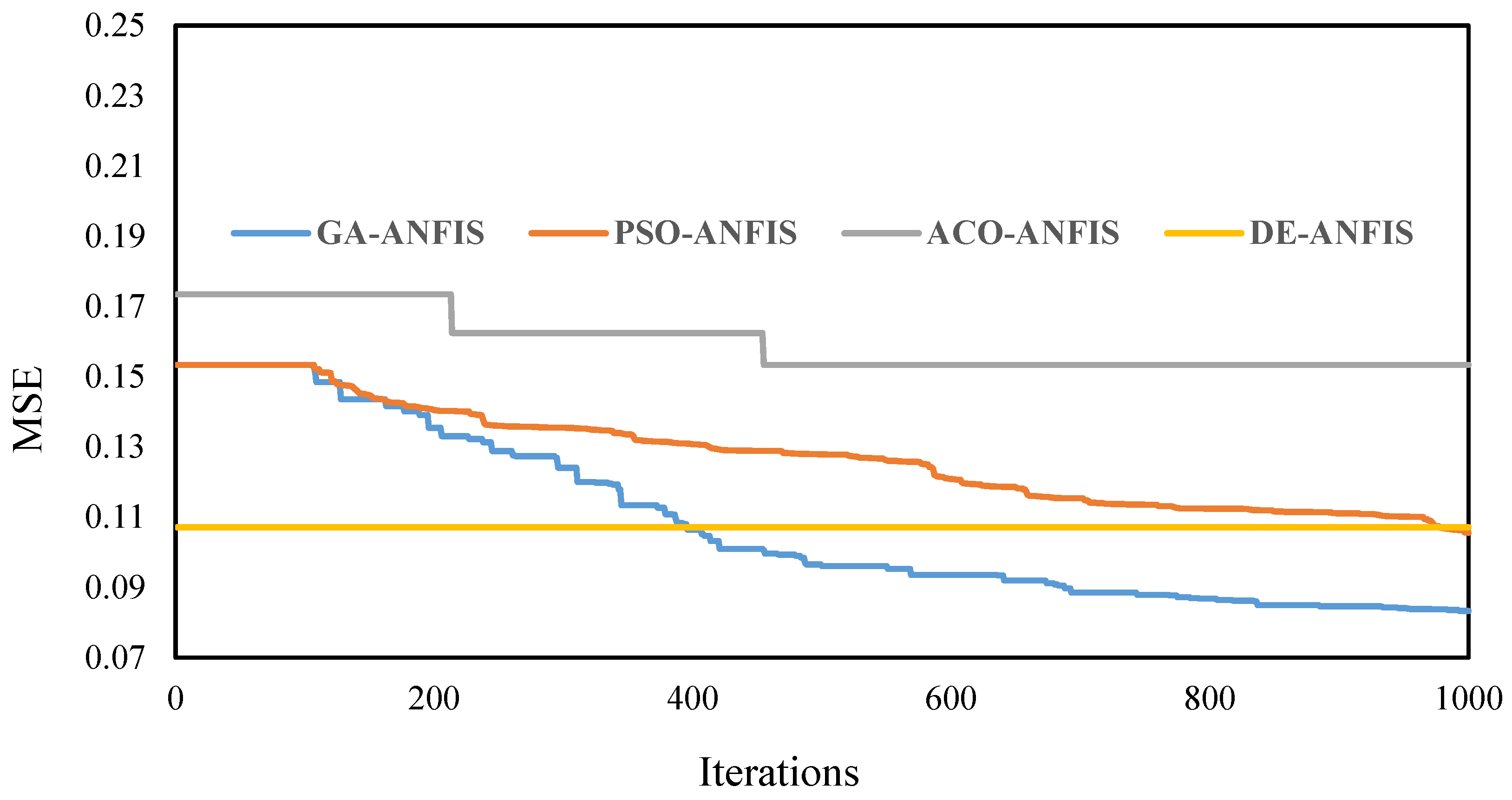
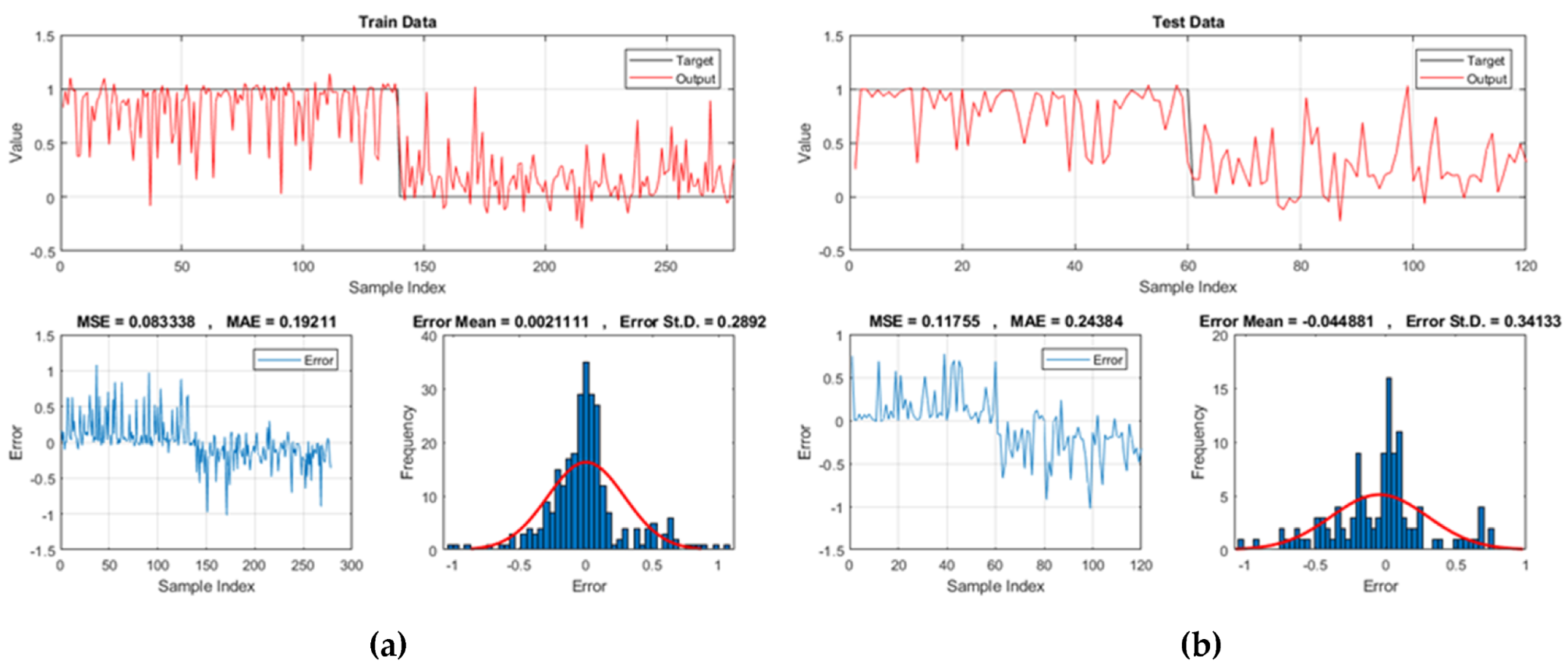
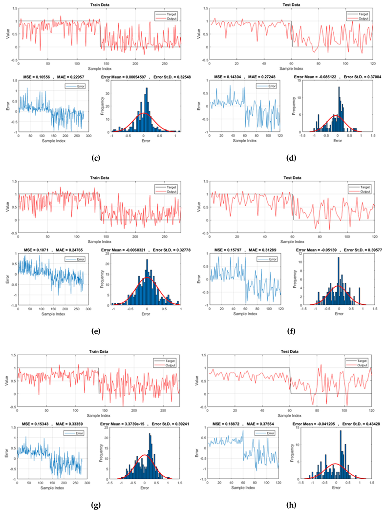
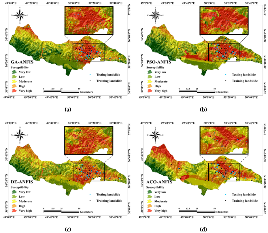
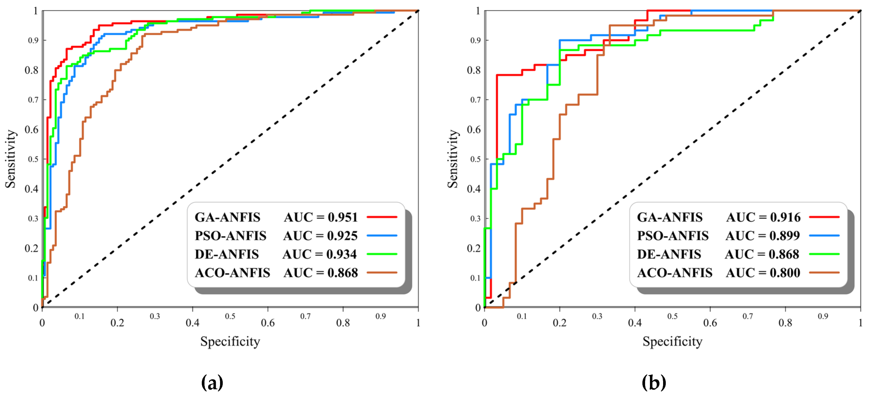
The primary version of ant colony optimization (ACO) method was known as the ant system which was first designed for optimizing the travelling salesman problem [69]. In fact, the main effort of this work is to find the shortest path to link the intended cities [70]. In the case of intelligent models, like ANN and ANFIS, this algorithm aims to achieve the optimal computational parameters of these networks. A presentable solution is made of some components which are added by ants in each iteration. The ants consider a probability for selecting these components. Two determinant factors in this process are the pheromone and the heuristic factors which respectively reflect the past experience of the relations and the tendency for choosing a component regarding the defined objective function (OF). In the ACO method, the shortest path is discovered by the artificial ants through leaving a chemical pheromone trail along the crossed path. They do this for guiding other relations. As a result, the most promising track is distinguished. Assuming τ i j α and η i j β as the pheromone value and heuristic factors, respectively, Equation (8) formulates the mentioned probability:
P i j q ( t ) = τ i j α × η i j β u N i q   τ i u α × η i u β ,
in which Ni defines a neighborhood of the node i.

3. Results

This paper investigates the efficiency of four evolutionary ensembles of a fuzzy-based model, namely GA-ANFIS, PSO-ANFIS, DE-ANFIS, and ACO-ANFIS for landslide susceptibility assessment. Qazvin County in Iran is selected as the study area. In this work, considering the common ratio of 70:30, 139 landslides were specified to the training phase, and the remaining 60 landslide points were used to measure the accuracy of the applied models. In the next step, four hybrid stochastic algorithms of GA, PSO, DE, and ACO were synthesized with the ANFIS predictive model for fine-tuning the ANFIS MFs [71]. In detail, when it comes to optimization algorithms, they need some computational parameters. Regarding the used basic model, these computational parameters can vary (e.g., the weights and biases in the ANNs). In the case of ANFIS, the mentioned optimization algorithms aim to find the optimal values for the parameters of MFs. Notably, ANFIS is known as a capable model due to having a combination of fuzzy inference system (FIS) expert knowledge and neural learning ability [34]. It has been promisingly used for landslide hazard analysis in previous researches [58,72]. At the beginning of the ANFIS performance, it constructs a basic FIS. The computational units are then extracted and updated by evolutionary algorithms. Eventually, they are applied to develop the optimized model.
The number of repetitions for all models determined as 1000 to give enough opportunity for decreasing the error. Meanwhile, the MSE between the actual and predicted landslide susceptibility indices were defined as the cost function. Figure 5 depicts the convergence diagram of the GA-ANFIS, PSO-ANFIS, DE-ANFIS, and ACO-ANFIS. As is seen, the algorithms have shown different behaviors for optimizing the ANFIS. The GA-ANFIS, as well as PSO-ANFIS, have started decreasing MSE after 100th iteration. The corresponding curves are on a continuously downward path. The GA-based ensemble surpasses the PSO-ANFIS and reaches a lower MSE in the final (0.08333771 vs. 0.105558762). Unlike these, the DE-ANFIS did not show any sensitivity to the number of iterations and remained steady till the end. The MSE for this model obtained 0.107146933 which shows a very close value to the cost function of the PSO-ANFIS. As for the ACO-ANFIS, it started with a relatively-high MSE and reduced it to 0.153427807 within three steps. All in all, DE-ANFIS can be introduced as the fastest ensemble.
The results of the training and testing performance of the models are presented in Figure 6 in three parts: (i) A graphical comparison between the actual (targets) and estimated (response) landslide susceptibility indices, (ii) A schematic view of the calculated error (i.e., the difference between the targets and system responses), and (iii) A histogram chart showing the frequency of each error value. To create the landslide susceptibility maps of the implemented models, the produced landslide susceptibility indices were extracted and inserted to ArcGIS. Additionally, Natural break classification method [73,74] was applied to classify the resulted maps into five susceptibility categories including Very-low, Low, Moderate, High, and Very-high susceptible.
Figure 7 shows the generated maps of the GA-ANFIS, PSO-ANFIS, DE-ANFIS, and ACO-ANFIS predictions.
As is seen, all four applied ensembles have rightly specified a high level of susceptibility to the areas with a large aggregation of the landslide points (see the marked area in Figure 7). In addition, they have fittingly classified the areas devoid of the landslide (mostly in the South and South-West of the studied area) as low and very low susceptible.
The percentage of each susceptibility map is also calculated. Accordingly, around 28% (1418 km2), 33% (1639 km2), 31% (1568 km2), and 46% (2315 km2) of the studied area is recognized to be under the high landslide occurrence risk (i.e., high and very high susceptibility classes), respectively from the side of GA-ANFIS, PSO-ANFIS, DE-ANFIS, and ACO-ANFIS ensembles. Besides, the largest percentage of the safe areas (very low and low categories) are obtained for the GA-ANFIS (15.48% and 30.82% respectively). The percentage of the training and testing landslide points located in each susceptibility class are also calculated and presented in Table 2. According to this table, 78.57%, 76.19%, 81.75%, and 88.10% of the training landslides, as well as 80.00%, 80.00%, 81.67%, and 93.33% of the testing landslides are rightly located in the landslide-prone areas by GA-ANFIS, PSO-ANFIS, DE-ANFIS, and ACO-ANFIS, respectively. Considerably, these values are obtained < 3% in the areas labeled as very low susceptibility.
For evaluating the accuracy of the generated landslide susceptibility maps, the ROC curve was plotted. As is known, the area under the ROC curve is a good accuracy indicator for diagnostic issues [75]. These value ranges from 0.5 to 1 so that the quality of the prediction is directly proportional to the AUROC value. The ROC curves of the implemented models are shown in Figure 8a,b, respectively, for the training and testing landslides.
The obtained values of all three accuracy criteria (i.e., MSE, MAE, and AUROC) are summarized in Table 3. A score-based ranking system is also developed within this table for better distinguish of the most capable model. Each accuracy criterion is considered for both training and testing phases to receive a ranking score varying between 1 to 4. In this regard, the more accuracy the index represents, the higher score is assigned to it. As is seen, in the training phase, the obtained MSEs and MAEs for GA-ANFIS (0.0833 and 0.1921), PSO-ANFIS (0.1055 and 0.2295), DE-ANFIS (0.1071 and 0.2476), and ACO-ANFIS (0.1534 and 0.3335) indicate a lower prediction error for the GA- and PSO-based ensembles. After those, the DE-based model outperformed the ACO-ANFIS. This claim can also be supported by respective calculated AUROCs 0.951, 0.925, 0.934, and 0.868. However, the AUROC of the DE-ANFIS is slightly higher than PSO-ANFIS.
The testing results show a good generalization power of all used models. Accordingly, the obtained MSEs and MAEs for GA-ANFIS (0.1175 and 0.2438), PSO-ANFIS (0.1430 and 0.2724), DE-ANFIS (0.1579 and 0.3128), and ACO-ANFIS (0.1887 and 0.3755) reveal that the first model has predicted the landslide hazard index more efficiently than other three models. Also, the PSO-ANFIS emerged as the second accurate model, followed by DE-ANFIS and ACO-ANFIS. Besides, the values of the AUROC represent 91.6%, 89.9%, 86.8%, and 80.0%. Prediction capability for the GA-ANFIS, PSO-ANFIS, DE-ANFIS, and ACO-ANFIS, respectively.
All in all, considering a total ranking score (TRS) as the summation of the scores obtained based on the mentioned indices, the GA-ANFIS (TRS = 24), emerged as the most promising model for spatial prediction of landslide hazard in the Qazvin county. After that, the PSO-ANFIS (TRS = 17), DE-ANFIS (TRS = 13), and ACO-ANFIS (TRS = 6) presented an acceptable prediction accuracy.

4. Discussion

Due to the devastating impacts of the landslides, susceptibility assessment of this natural hazard has received increasing attention during the last decades [76]. This study addresses the applicability evaluation of four hybrid integration techniques using the adaptive neuro-fuzzy inference system coupled with a genetic algorithm, particle swarm optimization, differential evolution and ant colony optimization for landslide susceptibility analysis in Qazvin Province (Iran). The prediction accuracy of the designed models was evaluated and compared using the ROC diagram and the AUROC index. As an advantage of the ANFIS, the basis of this predictive tool is a combination of neural learning of the ANNs and expert knowledge of FIS [34]. Some researchers have promisingly employed this model for landslide susceptibility mapping [34,77,78]. Oh and Pradhan [79] revealed that the ANFIS acts very effectively for regional assessment of landslide susceptibility. They tested various MFs embedded in this model for estimating the landslide susceptibility values in a prone district of Penang Island (Malaysia). The findings of the mentioned research demonstrated that the accuracy of the landslide susceptibility maps obtained from trapezoidal, triangular, polynomial and generalized bell MFs (accuracy ≈ 84%) surpass the ones produced by four different Gaussian and sigmoidal MFs.
As stated above, the ANFIS has emerged as one of the most powerful machine learning approaches, but some drawbacks associated with this tool (e.g., the non-adjutancy of membership) drive us to use hybrid evolutionary algorithms for optimizing its performance. In this paper, four wise optimization techniques of GA, PSO, DE, and ACO were applied to find the optimal values of the parameters of the ANFIS. More clearly, these algorithms are stochastic search schemes which perform in a repetitive loop to minimize a defined objective function. This process results in finding the most appropriate solution amongst a huge number of candidates.
The results indicated that all used models perform with good accuracy for the mentioned purpose. Having a look at the obtained accuracy criteria, as well as the spatial interaction between the landslide points and the susceptibility classes, it can be concluded that the GA-ANFIS (TRS = 24) excelled other designed ensembles. The PSO-ANFIS (TRS = 17) appeared to be the second accurate model, followed by the DE-ANFIS (TRS = 13) and ACO-ANFIS (TRS = 6). However, in similar research by Chen, Panahi and Pourghasemi [31], the superiority of the DE-based ensemble was stated (i.e., in comparison with PSO- and GA-based models), the outcomes of the present study confirm that the GA outperforms PSO for optimizing the parameters of the proposed fuzzy system. In fact, the discrete optimizing method of the GA surpassed the constant method of the PSO. More specifically, the latter algorithm allocates memory for maintaining every promising solution of all particles. This is while, prior knowledge of the GA population is antiquated as the new population is involved. Notably, the results of our study show more robustness in comparison with the mentioned reference.
Reaching the lowest training error (Figure 5) is, perhaps, the main reason for the excellent generalization power of the GA-ANFIS (91.6% accuracy). We say perhaps because despite a slightly smaller OF obtained for the PSO-ANFIS (0.1055) compared to DE-ANFIS (0.1071), it gave less training accuracy (92.5% vs. 93.4%). Moreover, not surprisingly, the appreciable distinction between the learning capability of the ACO-AFIS and other models (i.e., larger OF) led to weaker performance for estimating the landslide susceptibility values of the testing points. Altogether, there was no disagreement between the capability of learning a pattern and generalization power for all models used in this study. In other words, each model that excelled in the training phase, was superior in the testing phase, too.
Setting the performance of the applied algorithms aside, the number of iterations that each model needed to reach the lowest OF was considered as the main factor for evaluating the convergence speed of that model (i.e., within 1000 repetitions and regardless the time). It was deduced that the DE-ANFIS does not show any sensitivity to the number of repetitions, and the first try is the best one. It should be noted about DE that, unlike other metaheuristic techniques, the vectors of the current generation in this technique are created through random sampling and combining the vectors belonging to the former generation. Also, the real-valued mutation and crossover factors cause the convergence of the search action [80]. Similar to the ACO-ANFIS which Termeh, et al. [81] used for flood susceptibility modelling, it minimized the OF after a few major fluctuations. As for the PSO- and GA-based ensembles, both models continued decreasing the error until the end. Now, the main question is “which ensemble can be introduced as the most suitable model, considering both accuracy and time-effectiveness”? For answering this question, it should be mentioned that there is a nuance (0.0238 of MSE, 0.0555 of MAE, and 0.017 of AUROC) between the learning quality of the controversial models of this study (i.e., GA-ANFIS and DE-ANFIS). Hence, when the time comes out as a determinant factor, the DE-ANFIS is a more appropriate ensemble for landslide susceptibility assessment. In contrast, in cases that accuracy plays a more important role, utilizing the GA-ANFIS seems more reasonable.
The methodology proposed in this paper had some limitations too. Using the original input configuration (i.e., thirteen landslide conditioning factors) resulted in the generation of high-dimensionality networks which negatively influence the complexity and the computation time of the models. This issue can be solved by optimizing the input factors by metaheuristic schemes [28]. Also, taking the effect of other environmental parameters (e.g., local drainage networks) into account could be of interest for future studies. Moreover, referring to the convergence behavior of the elite models (i.e., the GA and PSO) in Figure 5, they are able to achieve more accurate understanding from the landslide pattern for further iterations. This is while this parameter was bound to 1000 in this study.

5. Conclusions

The importance of landslide susceptibility mapping for alleviating the damages triggered by this natural hazard is obvious. Due to the complexity and non-linearity of such modellings, the application of new intelligent tools like ANN and ANFIS has antiquated many traditional methods. Despite various benefits of these models, some difficulties like dimension dangers and local minimum still exist. Such problems have driven scholars to employ hybrid optimization algorithms for optimizing the performance of typical models, especially for high-dimensional problems like landslide susceptibility modelling. In the present study, firstly, the FR theory was used to assess the spatial interaction between the landslides and considered conditioning factors. Then, four wise metaheuristic algorithms, namely GA, PSO, DE, and ACO were employed to train the ANFIS, for proper landslide susceptibility analysis in Qazvin County (Iran). In fact, the main duty of the mentioned algorithms is to find the most appropriate computational parameters of the proposed fuzzy system, in order to decrease the impact of dimension dangers and local minimum. As the first outcome, the DE-ANFIS model emerged as the fastest ensemble for minimizing the OF. Eventually, the landside susceptibility maps were produced and the AUROC criterion was used to evaluate the accuracy of them. Referring to the obtained accuracies of 91.6%, 89.9%, 86.8%, and 80.0%, respectively for the GA-ANN, PSO-ANFIS, DE-ANFIS, and ACO-ANFIS ensembles, it was concluded that the GA outperforms other implemented algorithms in optimizing the performance of the ANFIS. The produced landslide susceptibility maps can be applied for proper decision making and risk management of landslide in the studied area. However, the results indicate that the designed models are accurate enough to be an alternative for the mentioned purpose, the authors believe that more accuracy can be achieved by applying various ideas such as simultaneous optimization of the input combination and the used predictive model, which seems a good subject for future studies.

Author Contributions

M.M. performed the experiments, wrote the manuscript, and collected the field data; M.M. wrote the manuscript and analyzed the data; B.P. supervised, edited, restructured, B.P. and B.P., A.A. and H.M. professionally optimized the manuscript; B.P. and A.A., including the funding acquisition. All authors have read and agreed to the published version of the manuscript.

Funding

This research is supported by the Centre for Advanced Modelling and Geospatial Information Systems (CAMGIS) in the University of Technology Sydney (UTS) under grant numbers: 323930, 321740.2232335; 321740.2232424 and 321740.2232357. This research was also supported by Researchers Supporting Project number RSP-2019/14, King Saud University, Riyadh, Saudi Arabia.

Conflicts of Interest

The authors declare that there is no conflict of interest.

References

  1. Varnes, D.; Radbruch-Hall, D. Landslides cause and effect. Bull. Int. Assoc. Eng. Geol. 1976, 13, 205–216. [Google Scholar]
  2. Pourghasemi, H.R.; Mohammady, M.; Pradhan, B. Landslide susceptibility mapping using index of entropy and conditional probability models in GIS: Safarood Basin, Iran. Catena 2012, 97, 71–84. [Google Scholar] [CrossRef]
  3. Shoaei, Z.; Ghayoumian, J. The largest debris flow in the world, Seimareh Landslide, Western Iran. In Environmental Forest Science; Springer: Berlin, Germany, 1998; pp. 553–561. [Google Scholar]
  4. Abdullahi, S.; Mahmud, A.R.B.; Pradhan, B. Spatial modelling of site suitability assessment for hospitals using geographical information system-based multicriteria approach at Qazvin city, Iran. Geocarto Int. 2014, 29, 164–184. [Google Scholar] [CrossRef]
  5. Hong, H.; Miao, Y.; Liu, J.; Zhu, A.X. Exploring the effects of the design and quantity of absence data on the performance of random forest-based landslide susceptibility mapping. CATENA 2019, 176, 45–64. [Google Scholar] [CrossRef]
  6. Moayedi, H.; Mehrabi, M.; Kalantar, B.; Abdullahi Mu’azu, M.; A. Rashid, A.S.; Foong, L.K.; Nguyen, H. Novel hybrids of adaptive neuro-fuzzy inference system (ANFIS) with several metaheuristic algorithms for spatial susceptibility assessment of seismic-induced landslide. Geomat. Nat. Hazards Risk 2019, 10, 1879–1911. [Google Scholar] [CrossRef] [Green Version]
  7. Bui, D.T.; Moayedi, H.; Kalantar, B.; Osouli, A.; Gör, M.; Pradhan, B.; Nguyen, H.; Rashid, A.S.A. Harris hawks optimization: A novel swarm intelligence technique for spatial assessment of landslide susceptibility. Sensors 2019, 19, 3590. [Google Scholar] [CrossRef] [Green Version]
  8. Xiao, T.; Yin, K.; Yao, T.; Liu, S. Spatial prediction of landslide susceptibility using GIS-based statistical and machine learning models in Wanzhou County, Three Gorges Reservoir, China. Acta Geochim. 2019, 38, 654–669. [Google Scholar] [CrossRef]
  9. Razavizadeh, S.; Solaimani, K.; Massironi, M.; Kavian, A. Mapping landslide susceptibility with frequency ratio, statistical index, and weights of evidence models: A case study in northern Iran. Environ. Earth Sci. 2017, 76, 499. [Google Scholar] [CrossRef]
  10. Youssef, A.M.; Al-Kathery, M.; Pradhan, B. Landslide susceptibility mapping at Al-Hasher area, Jizan (Saudi Arabia) using GIS-based frequency ratio and index of entropy models. Geosci. J. 2015, 19, 113–134. [Google Scholar] [CrossRef]
  11. Nicu, I.C.; Asăndulesei, A. GIS-based evaluation of diagnostic areas in landslide susceptibility analysis of Bahluieț River Basin (Moldavian Plateau, NE Romania). Are Neolithic sites in danger? Geomorphology 2018, 314, 27–41. [Google Scholar] [CrossRef]
  12. Fayez, L.; Pazhman, D.; Pham, B.T.; Dholakia, M.; Solanki, H.; Khalid, M.; Prakash, I. Application of Frequency Ratio Model for the Development of Landslide Susceptibility Mapping at Part of Uttarakhand State, India. Int. J. Appl. Eng. Res. 2018, 13, 6846–6854. [Google Scholar]
  13. Chen, W.; Chai, H.; Sun, X.; Wang, Q.; Ding, X.; Hong, H. A GIS-based comparative study of frequency ratio, statistical index and weights-of-evidence models in landslide susceptibility mapping. Arab. J. Geosci. 2016, 9, 204. [Google Scholar] [CrossRef]
  14. Bahrami, Y.; Hassani, H.; Maghsoudi, A. Landslide susceptibility mapping using AHP and fuzzy methods in the Gilan province, Iran. GeoJournal 2020, 1–20. [Google Scholar] [CrossRef]
  15. El Jazouli, A.; Barakat, A.; Khellouk, R. GIS-multicriteria evaluation using AHP for landslide susceptibility mapping in Oum Er Rbia high basin (Morocco). Geoenviron. Disasters 2019, 6, 3. [Google Scholar] [CrossRef]
  16. Yan, F.; Zhang, Q.; Ye, S.; Ren, B. A novel hybrid approach for landslide susceptibility mapping integrating analytical hierarchy process and normalized frequency ratio methods with the cloud model. Geomorphology 2019, 327, 170–187. [Google Scholar] [CrossRef]
  17. Yang, J.; Song, C.; Yang, Y.; Xu, C.; Guo, F.; Xie, L. New method for landslide susceptibility mapping supported by spatial logistic regression and GeoDetector: A case study of Duwen Highway Basin, Sichuan Province, China. Geomorphology 2019, 324, 62–71. [Google Scholar] [CrossRef]
  18. Liu, J.; Duan, Z. Quantitative assessment of landslide susceptibility comparing statistical index, index of entropy, and weights of evidence in the Shangnan area, China. Entropy 2018, 20, 868. [Google Scholar] [CrossRef] [Green Version]
  19. Yang, Y.; Yang, J.; Xu, C.; Xu, C.; Song, C. Local-scale landslide susceptibility mapping using the B-GeoSVC model. Landslides 2019, 16, 1301–1312. [Google Scholar] [CrossRef]
  20. Pradhan, B.; Lee, S. Regional landslide susceptibility analysis using back-propagation neural network model at Cameron Highland, Malaysia. Landslides 2010, 7, 13–30. [Google Scholar] [CrossRef]
  21. Chen, W.; Pourghasemi, H.R.; Naghibi, S.A. A comparative study of landslide susceptibility maps produced using support vector machine with different kernel functions and entropy data mining models in China. Bull. Eng. Geol. Environ. 2018, 77, 647–664. [Google Scholar] [CrossRef]
  22. Vahidnia, M.H.; Alesheikh, A.A.; Alimohammadi, A.; Hosseinali, F. A GIS-based neuro-fuzzy procedure for integrating knowledge and data in landslide susceptibility mapping. Comput. Geosci. 2010, 36, 1101–1114. [Google Scholar] [CrossRef]
  23. Aditian, A.; Kubota, T.; Shinohara, Y. Comparison of GIS-based landslide susceptibility models using frequency ratio, logistic regression, and artificial neural network in a tertiary region of Ambon, Indonesia. Geomorphology 2018, 318, 101–111. [Google Scholar] [CrossRef]
  24. Polykretis, C.; Chalkias, C.; Ferentinou, M. Adaptive neuro-fuzzy inference system (ANFIS) modeling for landslide susceptibility assessment in a Mediterranean hilly area. Bull. Eng. Geol. Environ. 2019, 78, 1173–1187. [Google Scholar] [CrossRef]
  25. Chen, W.; Pourghasemi, H.R.; Panahi, M.; Kornejady, A.; Wang, J.; Xie, X.; Cao, S. Spatial prediction of landslide susceptibility using an adaptive neuro-fuzzy inference system combined with frequency ratio, generalized additive model, and support vector machine techniques. Geomorphology 2017, 297, 69–85. [Google Scholar] [CrossRef]
  26. Pham, B.T.; Shirzadi, A.; Bui, D.T.; Prakash, I.; Dholakia, M. A hybrid machine learning ensemble approach based on a radial basis function neural network and rotation forest for landslide susceptibility modeling: A case study in the Himalayan area, India. Int. J. Sediment Res. 2018, 33, 157–170. [Google Scholar] [CrossRef]
  27. Jaafari, A.; Panahi, M.; Pham, B.T.; Shahabi, H.; Bui, D.T.; Rezaie, F.; Lee, S. Meta optimization of an adaptive neuro-fuzzy inference system with grey wolf optimizer and biogeography-based optimization algorithms for spatial prediction of landslide susceptibility. Catena 2019, 175, 430–445. [Google Scholar] [CrossRef]
  28. Li, L.; Liu, R.; Pirasteh, S.; Chen, X.; He, L.; Li, J. A novel genetic algorithm for optimization of conditioning factors in shallow translational landslides and susceptibility mapping. Arab. J. Geosci. 2017, 10, 209. [Google Scholar] [CrossRef]
  29. Tien Bui, D.; Pham, B.T.; Nguyen, Q.P.; Hoang, N.-D. Spatial prediction of rainfall-induced shallow landslides using hybrid integration approach of Least-Squares Support Vector Machines and differential evolution optimization: A case study in Central Vietnam. Int. J. Digit. Earth 2016, 9, 1077–1097. [Google Scholar] [CrossRef]
  30. Nguyen, H.; Mehrabi, M.; Kalantar, B.; Moayedi, H.; Abdullahi, M.a.M. Potential of hybrid evolutionary approaches for assessment of geo-hazard landslide susceptibility mapping. Geomat. Nat. Hazards Risk 2019, 10, 1667–1693. [Google Scholar] [CrossRef]
  31. Chen, W.; Panahi, M.; Pourghasemi, H.R. Performance evaluation of GIS-based new ensemble data mining techniques of adaptive neuro-fuzzy inference system (ANFIS) with genetic algorithm (GA), differential evolution (DE), and particle swarm optimization (PSO) for landslide spatial modelling. Catena 2017, 157, 310–324. [Google Scholar] [CrossRef]
  32. Tien Bui, D.; Shahabi, H.; Shirzadi, A.; Chapi, K.; Hoang, N.-D.; Pham, B.; Bui, Q.-T.; Tran, C.-T.; Panahi, M.; Bin Ahamd, B. A novel integrated approach of relevance vector machine optimized by imperialist competitive algorithm for spatial modeling of shallow landslides. Remote Sens. 2018, 10, 1538. [Google Scholar] [CrossRef] [Green Version]
  33. Ghorbanzadeh, O.; Rostamzadeh, H.; Blaschke, T.; Gholaminia, K.; Aryal, J. A new GIS-based data mining technique using an adaptive neuro-fuzzy inference system (ANFIS) and k-fold cross-validation approach for land subsidence susceptibility mapping. Nat. Hazards 2018, 94, 497–517. [Google Scholar] [CrossRef] [Green Version]
  34. Lee, M.-J.; Park, I.; Lee, S. Forecasting and validation of landslide susceptibility using an integration of frequency ratio and neuro-fuzzy models: a case study of Seorak mountain area in Korea. Environ. Earth Sci. 2015, 74, 413–429. [Google Scholar] [CrossRef]
  35. Ahmadlou, M.; Karimi, M.; Alizadeh, S.; Shirzadi, A.; Parvinnejhad, D.; Shahabi, H.; Panahi, M. Flood susceptibility assessment using integration of adaptive network-based fuzzy inference system (ANFIS) and biogeography-based optimization (BBO) and BAT algorithms (BA). Geocarto Int. 2018, 1–21. [Google Scholar] [CrossRef]
  36. Moayedi, H.; Mehrabi, M.; Bui, D.T.; Pradhan, B.; Foong, L.K. Fuzzy-metaheuristic ensembles for spatial assessment of forest fire susceptibility. J. Environ. Manag. 2020, 109867. [Google Scholar] [CrossRef] [PubMed]
  37. Chen, W.; Panahi, M.; Tsangaratos, P.; Shahabi, H.; Ilia, I.; Panahi, S.; Li, S.; Jaafari, A.; Ahmad, B.B. Applying population-based evolutionary algorithms and a neuro-fuzzy system for modeling landslide susceptibility. Catena 2019, 172, 212–231. [Google Scholar] [CrossRef]
  38. Moayedi, H.; Mehrabi, M.; Mosallanezhad, M.; Rashid, A.S.A.; Pradhan, B. Modification of landslide susceptibility mapping using optimized PSO-ANN technique. Eng. Comput. 2019, 35, 967–984. [Google Scholar] [CrossRef]
  39. Shahrood (River). Available online: https://en.wikipedia.org/wiki/Shahrood_(River) (accessed on 6 March 2020).
  40. Shemshad, K.; Rafinejad, J.; Kamali, K.; Piazak, N.; Sedaghat, M.M.; Shemshad, M.; Biglarian, A.; Nourolahi, F.; Beigi, E.V.; Enayati, A.A. Species diversity and geographic distribution of hard ticks (Acari: Ixodoidea: Ixodidae) infesting domestic ruminants, in Qazvin Province, Iran. Parasitol. Res. 2012, 110, 373–380. [Google Scholar] [CrossRef]
  41. Pradhan, B. A comparative study on the predictive ability of the decision tree, support vector machine and neuro-fuzzy models in landslide susceptibility mapping using GIS. Comput. Geosci. 2013, 51, 350–365. [Google Scholar] [CrossRef]
  42. Vakhshoori, V.; Pourghasemi, H.R. A novel hybrid bivariate statistical method entitled FROC for landslide susceptibility assessment. Environ. Earth Sci. 2018, 77, 686. [Google Scholar] [CrossRef]
  43. Pradhan, B.; Lee, S.; Buchroithner, M.F. A GIS-based back-propagation neural network model and its cross-application and validation for landslide susceptibility analyses. Comput. Environ. Urban Syst. 2010, 34, 216–235. [Google Scholar] [CrossRef]
  44. Shirzadi, A.; Bui, D.T.; Pham, B.T.; Solaimani, K.; Chapi, K.; Kavian, A.; Shahabi, H.; Revhaug, I. Shallow landslide susceptibility assessment using a novel hybrid intelligence approach. Environ. Earth Sci. 2017, 76, 60. [Google Scholar] [CrossRef]
  45. Guzzetti, F.; Mondini, A.C.; Cardinali, M.; Fiorucci, F.; Santangelo, M.; Chang, K.-T. Landslide inventory maps: New tools for an old problem. Earth Sci. Rev. 2012, 112, 42–66. [Google Scholar] [CrossRef] [Green Version]
  46. Pourghasemi, H.R.; Jirandeh, A.G.; Pradhan, B.; Xu, C.; Gokceoglu, C. Landslide susceptibility mapping using support vector machine and GIS at the Golestan Province, Iran. J. Earth Syst. Sci. 2013, 122, 349–369. [Google Scholar] [CrossRef] [Green Version]
  47. Arjmandzadeh, R.; Teshnizi, E.S.; Rastegarnia, A.; Golian, M.; Jabbari, P.; Shamsi, H.; Tavasoli, S. GIS-Based Landslide Susceptibility Mapping in Qazvin Province of Iran. Iran. J. Sci. Techno. Trans. Civil Eng. 2019, 1–29. [Google Scholar] [CrossRef]
  48. Oh, H.-J.; Kim, Y.-S.; Choi, J.-K.; Park, E.; Lee, S. GIS mapping of regional probabilistic groundwater potential in the area of Pohang City, Korea. J. Hydrol. 2011, 399, 158–172. [Google Scholar] [CrossRef]
  49. Pourghasemi, H.; Moradi, H.; Aghda, S.F. Landslide susceptibility mapping by binary logistic regression, analytical hierarchy process, and statistical index models and assessment of their performances. Nat. hazards 2013, 69, 749–779. [Google Scholar] [CrossRef]
  50. Moayedi, H.; Hayati, S. Modelling and optimization of ultimate bearing capacity of strip footing near a slope by soft computing methods. Appl. Soft Comput. 2018, 66, 208–219. [Google Scholar] [CrossRef]
  51. Yilmaz, I. Landslide susceptibility mapping using frequency ratio, logistic regression, artificial neural networks and their comparison: a case study from Kat landslides (Tokat—Turkey). Comput. Geosci. 2009, 35, 1125–1138. [Google Scholar] [CrossRef]
  52. Shirzadi, A.; Soliamani, K.; Habibnejhad, M.; Kavian, A.; Chapi, K.; Shahabi, H.; Chen, W.; Khosravi, K.; Thai Pham, B.; Pradhan, B. Novel GIS based machine learning algorithms for shallow landslide susceptibility mapping. Sensors 2018, 18, 3777. [Google Scholar] [CrossRef]
  53. Pourghasemi, H.R.; Kerle, N. Random forests and evidential belief function-based landslide susceptibility assessment in Western Mazandaran Province, Iran. Environ. Earth Sci. 2016, 75, 185. [Google Scholar] [CrossRef]
  54. Zare, M.; Pourghasemi, H.R.; Vafakhah, M.; Pradhan, B. Landslide susceptibility mapping at Vaz Watershed (Iran) using an artificial neural network model: A comparison between multilayer perceptron (MLP) and radial basic function (RBF) algorithms. Arab. J. GeoL. 2013, 6, 2873–2888. [Google Scholar] [CrossRef]
  55. BEVEN, K.J.; Kirkby, M.J. A physically based, variable contributing area model of basin hydrology/Un modèle à base physique de zone d’appel variable de l’hydrologie du bassin versant. Hydrol. Sci. J. 1979, 24, 43–69. [Google Scholar] [CrossRef] [Green Version]
  56. Moore, I.D.; Grayson, R.; Ladson, A. Digital terrain modelling: a review of hydrological, geomorphological, and biological applications. Hydrol. Process. 1991, 5, 3–30. [Google Scholar] [CrossRef]
  57. Jang, J.-S. ANFIS: adaptive-network-based fuzzy inference system. IEEE Trans. Syst. Man Cybern. 1993, 23, 665–685. [Google Scholar] [CrossRef]
  58. Dehnavi, A.; Aghdam, I.N.; Pradhan, B.; Varzandeh, M.H.M. A new hybrid model using step-wise weight assessment ratio analysis (SWARA) technique and adaptive neuro-fuzzy inference system (ANFIS) for regional landslide hazard assessment in Iran. Catena 2015, 135, 122–148. [Google Scholar] [CrossRef]
  59. Nguyen, H.T.; Prasad, N.R.; Walker, E.A.; Walker, C.L. A First Course in Fuzzy and Neural Control; Chapman and Hall/CRC: Boca Raton, FL, USA, 2002. [Google Scholar]
  60. Holland, J.H. Adaptation in Natural and Artificial Systems: An Introductory Analysis with Applications to Biology, Control, and Artificial Intelligence; University of Michigan press Ann Arbor: Ann Arbor, MI, USA, 1975. [Google Scholar]
  61. Pham, D.; Karaboga, D. Optimum design of fuzzy logic controllers using genetic algorithms. J. Syst. Eng. 1991, 1, 114–118. [Google Scholar]
  62. Kennedy, J.; Eberhart, R. Particle swarm optimization. In Proceedings of the ICNN’95-International Conference on Neural Networks, Perth, Australia, 27 November–1 December 1995; Volume 1944, pp. 1942–1948. [Google Scholar]
  63. Kennedy, J. Particle swarm optimization. Encycl. Mach. Learn. 2010, 760–766. [Google Scholar]
  64. Poli, R.; Kennedy, J.; Blackwell, T. Particle swarm optimization. Swarm Intell. 2007, 1, 33–57. [Google Scholar] [CrossRef]
  65. Storn, R.; Price, K. Differential evolution–a simple and efficient heuristic for global optimization over continuous spaces. J. Glob. Optim. 1997, 11, 341–359. [Google Scholar] [CrossRef]
  66. Storn, R. Differential evolution research–trends and open questions. In Advances in Differential Evolution; Springer: Berlin, Germany, 2008; pp. 1–31. [Google Scholar]
  67. Abdul-Rahman, O.A.; Munetomo, M.; Akama, K. An adaptive parameter binary-real coded genetic algorithm for constraint optimization problems: Performance analysis and estimation of optimal control parameters. Inf. Sci. 2013, 233, 54–86. [Google Scholar] [CrossRef]
  68. Zheng, Q.; Simon, D.; Richter, H.; Gao, Z. Differential particle swarm evolution for robot control tuning. In Proceedings of the American Control Conference (ACC), Portland, OR, USA, 4–6 June 2014; pp. 5276–5281. [Google Scholar]
  69. Dorigo, M. Optimization, Learning and Natural Algorithms. Ph.D. Thesis, Politecnico di Milano, Milano, Italy, 1992. [Google Scholar]
  70. Castillo, O.; Neyoy, H.; Soria, J.; Melin, P.; Valdez, F. A new approach for dynamic fuzzy logic parameter tuning in ant colony optimization and its application in fuzzy control of a mobile robot. Appl. Soft Comput. 2015, 28, 150–159. [Google Scholar] [CrossRef]
  71. Mahapatra, S.; Daniel, R.; Dey, D.N.; Nayak, S.K. Induction motor control using PSO-ANFIS. Procedia Comput. Sci. 2015, 48, 753–768. [Google Scholar] [CrossRef] [Green Version]
  72. Aghdam, I.N.; Varzandeh, M.H.M.; Pradhan, B. Landslide susceptibility mapping using an ensemble statistical index (Wi) and adaptive neuro-fuzzy inference system (ANFIS) model at Alborz Mountains (Iran). Environ. Earth Sci. 2016, 75, 553. [Google Scholar] [CrossRef]
  73. Pourghasemi, H.; Pradhan, B.; Gokceoglu, C.; Moezzi, K.D. A comparative assessment of prediction capabilities of Dempster–Shafer and weights-of-evidence models in landslide susceptibility mapping using GIS. Geomat. Nat. Hazards Risk 2013, 4, 93–118. [Google Scholar] [CrossRef]
  74. Xu, C.; Dai, F.; Xu, X.; Lee, Y.H. GIS-based support vector machine modeling of earthquake-triggered landslide susceptibility in the Jianjiang River watershed, China. Geomorphology 2012, 145, 70–80. [Google Scholar] [CrossRef]
  75. Egan, J.P. Signal Detection Theory and {ROC} Analysis; Academic press: Cambridge, MA, USA, 1975. [Google Scholar]
  76. Süzen, M.L.; Doyuran, V. Data driven bivariate landslide susceptibility assessment using geographical information systems: a method and application to Asarsuyu catchment, Turkey. Eng. Geol. 2004, 71, 303–321. [Google Scholar] [CrossRef]
  77. Bui, D.T.; Pradhan, B.; Lofman, O.; Revhaug, I.; Dick, O.B. Landslide susceptibility mapping at Hoa Binh province (Vietnam) using an adaptive neuro-fuzzy inference system and GIS. Comput. Geosci. 2012, 45, 199–211. [Google Scholar]
  78. Sezer, E.A.; Pradhan, B.; Gokceoglu, C. Manifestation of an adaptive neuro-fuzzy model on landslide susceptibility mapping: Klang valley, Malaysia. Expert Syst. Appl. 2011, 38, 8208–8219. [Google Scholar] [CrossRef]
  79. Oh, H.-J.; Pradhan, B. Application of a neuro-fuzzy model to landslide-susceptibility mapping for shallow landslides in a tropical hilly area. Comput. Geosci. 2011, 37, 1264–1276. [Google Scholar] [CrossRef]
  80. Das, S.K.; Biswal, R.K.; Sivakugan, N.; Das, B. Classification of slopes and prediction of factor of safety using differential evolution neural networks. Environ. Earth Sci. 2011, 64, 201–210. [Google Scholar] [CrossRef]
  81. Termeh, S.V.R.; Kornejady, A.; Pourghasemi, H.R.; Keesstra, S. Flood susceptibility mapping using novel ensembles of adaptive neuro fuzzy inference system and metaheuristic algorithms. Sci. Total Environ. 2018, 615, 438–451. [Google Scholar] [CrossRef] [PubMed]
Figure 1. Location of the study area, and spatial distribution of landslides and non-landslide points.
Sensors 20 01723 g001
Figure 2. Landslide conditioning factor, percentage of the area for each sub-class, and the calculated FR for: (a) elevation, (b) slope aspect, (c) climate, (d) plan curvature, (e) soil type, (f) lithology, (g) distance to river, (h) distance to road, (i) distance to fault, (j) land cover, (k) slope degree, (l) SPI, and (m) TWI.
Sensors 20 01723 g002aSensors 20 01723 g002bSensors 20 01723 g002c
Figure 3. The obtained FRs for landslide conditioning factors: (a) elevation, (b) slope aspect, (c) climate, (d) plan curvature, (e) soil type, (f) distance to river, (g) distance to road, (h) distance to fault, (i) land cover, (j) slope degree, (k) SPI, and (l) TWI.
Sensors 20 01723 g003aSensors 20 01723 g003bSensors 20 01723 g003c
Figure 4. The methodology of the applied procedure for landslide susceptibility assessment.
Sensors 20 01723 g004
Figure 5. The convergence curves of the cost functions for the used models.
Sensors 20 01723 g005
Figure 6. The results obtained for (a) and (b) GA-ANFIS, (c) and (d) PSO-ANFIS, (e) and (f) DE-ANFIS, (g) and (h) ACO-ANFIS, respectively for the training and testing samples.
Sensors 20 01723 g006aSensors 20 01723 g006b
Figure 7. Generated landslide susceptibility maps for (a) GA-ANFIS, (b) PSO-ANFIS, (c) DE-ANFIS, (d) ACO-ANFIS.
Sensors 20 01723 g007
Figure 8. Obtained for the (a) training data and (b) testing data.
Sensors 20 01723 g008
Table 1. The description of the lithology units.
NameSymbolDescriptionGeological AgeAge EraFR
AQft1Vally terrace deposits and high level piedmont fanQuaternaryCenozoic0.1342
BMm,s,lCalcareous sandstone, Marl, sandy limestone, and minor conglomerateMioceneCenozoic1.8086
CEkWell bedded green tuff and tuffaceous shale (KARAJ FM)EoceneCenozoic1.8527
DEbvBasaltic volcanic rocksMiddle. EoceneCenozoic1.4191
EEk.aCalcareous shale with subordinate tuff (Asara Shale)Middle. EoceneCenozoic0.0000
FPrDark grey medium-bedded to massive limestone (RUTEH LIMESTONE)PermianPaleozoic0.9016
GTRJsDark grey shale and sandstone (SHEMSHAK FM.)Triassic-JurassicMesozoic5.8083
HEkshGreenish-black shale and partly tuffaceous with intercalations of tuff (Lower Shale Member)Middle. EoceneCenozoic0.0000
IQft2Low level piedment fan and vally terrace depositsQuaternaryCenozoic0.9509
GEdavtDacitic andesitic volcanic tuffMiddle-Late. EoceneCenozoic0.1144
KPgkcLight-red coarse grained, and polygenic conglomerate with sandstone intercalationsPaleocene-EoceneCenozoic1.0196
LOgr-diGranite to dioriteOligoceneCenozoic0.0000
MEavAndesitic volcanicsMiddle. EoceneCenozoic0.8304
NKbvBasaltic volcanicEarly. CretaceousMesozoic0.0000
OKtzlThick bedded to massive, and white to pinkish orbitolina bearing limestone (TIZKUH FM)Early. CretaceousMesozoic0.0000
PTReThick bedded grey o’olitic limestone, thin-platy, yellow to pinkish shaly limestone with worm tracks and well to thick-bedded dolomite and dolomitic limestone (ELIKAH FM.)Early-Middle. TriassicMesozoic0.0111
QgbGabbroEoceneCenozoic5.5427
REdavDacitic to Andesitic volcanicEoceneCenozoic0.4563
SCbLimestone, alternation of dolomite, and verigated shale (BARUT FM)CambrianPaleozoic0.0000
TJlLight grey, and thin-bedded to massive limestone (LAR FM)Jurassic-CretaceousMesozoic3.5884
UEdtRhyolitic to rhyodacitic tuffEoceneCenozoic2.6755
VQabvAndesite to basaltic volcanicsQuaternaryCenozoic0.2398
WOdiDioriteOligoceneCenozoic0.7280
XEkgyGypsumLate. EoceneCenozoic0.0000
YEbtBasaltic tuffEoceneCenozoic0.0000
Table 2. The percentage of the training and testing landslides in each susceptibility classes.
Susceptibility
Class
GA-ANFISPSO-ANFISDE-ANFISACO-ANFIS
TrainTestTrainTestTrainTestTrainTest
Very low1.510.000.910.000.000.001.160.00
Low4.494.142.980.002.522.991.821.99
Moderate11.8510.437.400.5011.437.5210.104.06
High14.039.9713.671.3122.3719.7932.9233.36
Very high68.1375.4675.0498.1963.6769.7154.0060.58
Table 3. The ranking system based on the results of the spatial prediction of landslide susceptibility.
Ensemble ModelsNetwork ResultsRanking ScoreTotal Ranking Score (TRS)Rank
Training PhaseTesting PhaseTraining PhaseTesting Phase
MSEMAEAUROCMSEMAEAUROCMSEMAEAUROCMSEMAEAUROC
GA-ANFIS0.08330.19210.9510.11750.24380.916444444241
PSO-ANFIS0.10550.22950.9250.14300.27240.899332333172
DE-ANFIS0.10710.24760.9340.15790.31280.868223222133
ACO-ANFIS0.15340.33350.8680.18870.37550.80011111164

