VersaVIS—An Open Versatile Multi-Camera Visual-Inertial Sensor Suite

 , , , , , , , and
Abstract
1. Introduction
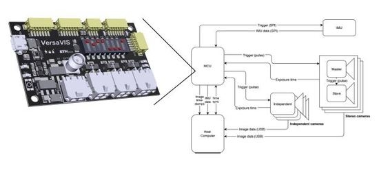
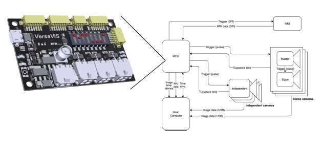
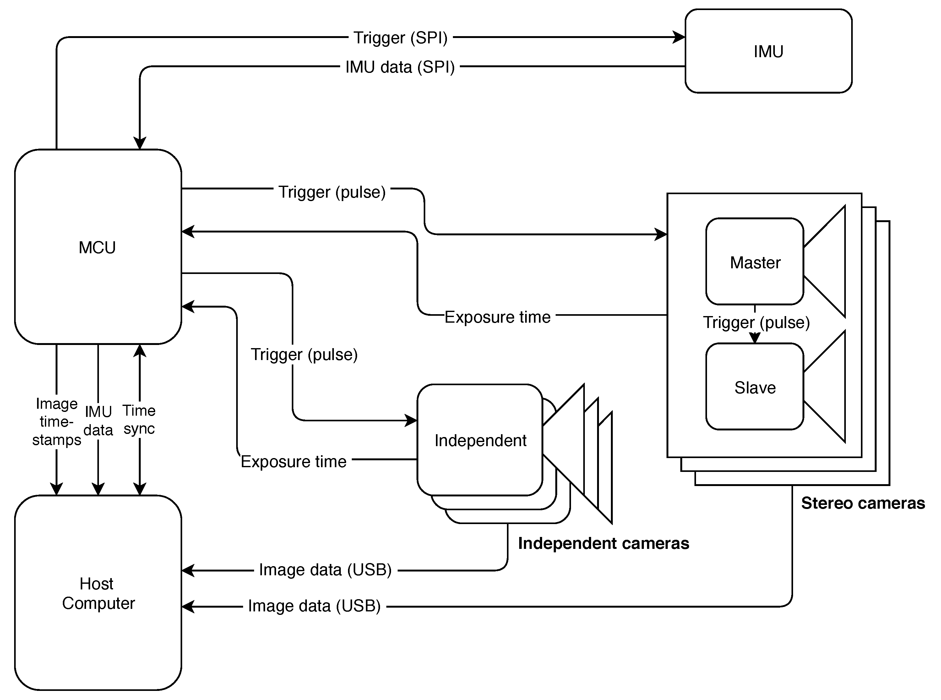
2. The Visual-Inertial Sensor Suite
2.1. Firmware
2.1.1. Standard Cameras
- Initialization procedure: After startup of the camera and trigger board, corresponding sequence numbers are found by very slowly triggering the camera without exposure time compensation. Corresponding sequence numbers are then determined by closest timestamps, see Section 2.2.1. This holds true if the triggering period time is significantly longer than the expected delay and jitter on the host computer. As soon as the sequence number offset is determined, exposure compensation mode at full frame rate can be used.
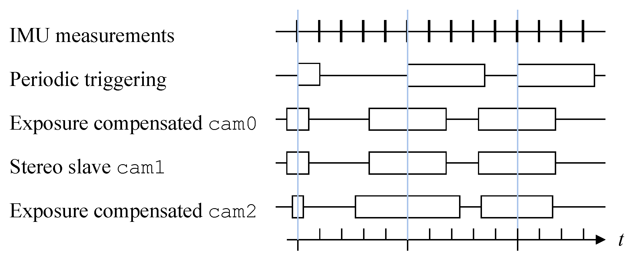
- Exposure time compensation: Performing auto-exposure (AE), the camera adapts its exposure time to the current illumination resulting in a non-constant exposure time. Furgale et al. [22] showed, that mid-exposure timestamping is beneficial for image based state estimation, especially when using global shutter cameras. Instead of periodically triggering the camera, a scheme proposed by Nikolic et al. [9] is employed. The idea is to trigger the camera for a periodic mid-exposure timestamp by starting exposure half the exposure time earlier to its mid-exposure timestamp as shown in Figure 3 for cam0, cam1 and cam2. The exposure time return signal is used to time the current exposure time and calculate the offset to the mid-exposure timestamp of the next image. Using this approach, corresponding measurements can be obtained even if multiple cameras do not share the same exposure time (e.g., cam0 and cam2 in Figure 3).
- Master-slave mode: Using two cameras in a stereo setup compared to a monocular camera can retrieve metric scale by stereo matching. This can enable certain applications where IMU excitation is not high enough and therefore biases are not fully observable without this scale input for example, for rail vehicles described in Section 4.2. Furthermore, it can also provide more robustness. To perform accurate and efficient stereo matching, it is highly beneficial if keypoints from the same spot have a similar appearance. This can be achieved by using the exact same exposure time on both cameras. Thereby, one camera serves as the master performing AE while the other adapts its exposure time. This is achieved by routing the exposure signal from cam0 directly to the trigger of cam1 and also using it to determine the exposure time for compensation.
2.1.2. Other Triggerable Sensors
2.1.3. Other Non-Triggerable Sensors
2.2. Host Computer Driver
2.2.1. Synchronizer
2.2.2. IMU Receiver
2.3. VersaVIS Triggering Board
3. Evaluations
3.1. Camera-Camera
3.2. Camera-IMU
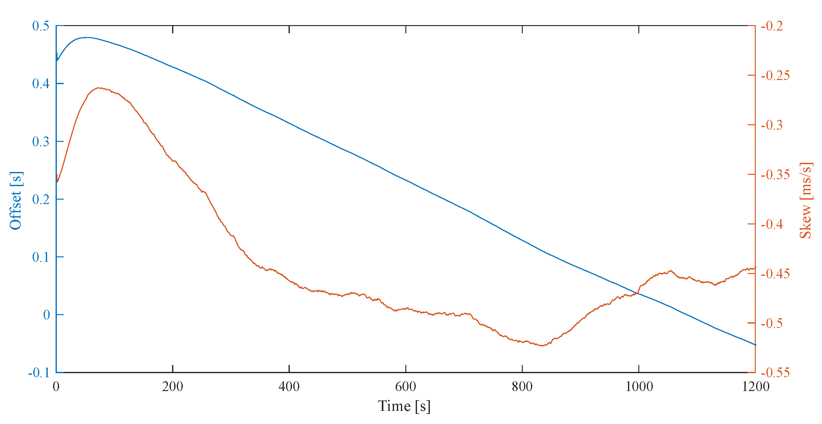
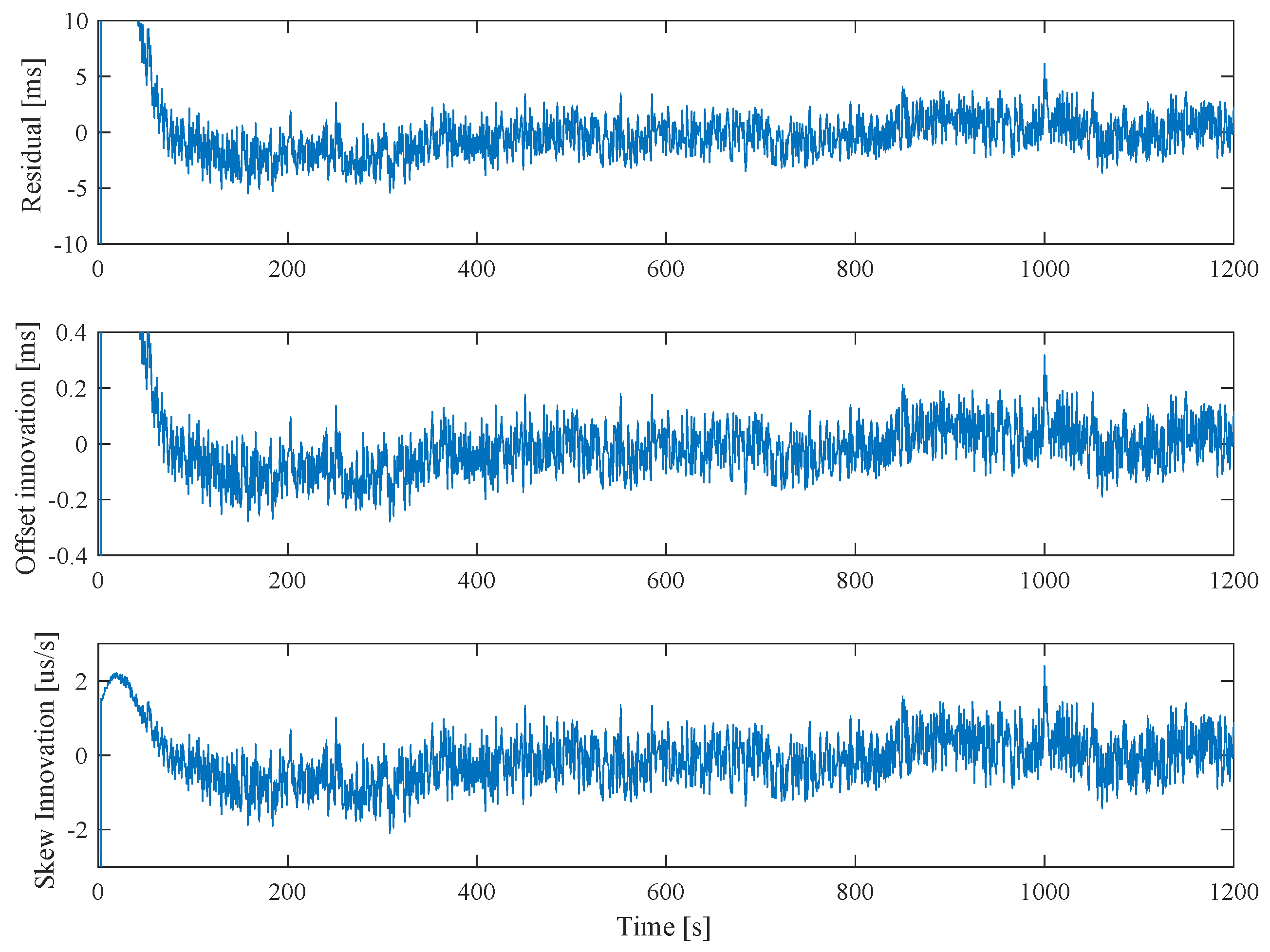
3.3. VersaVIS-Host
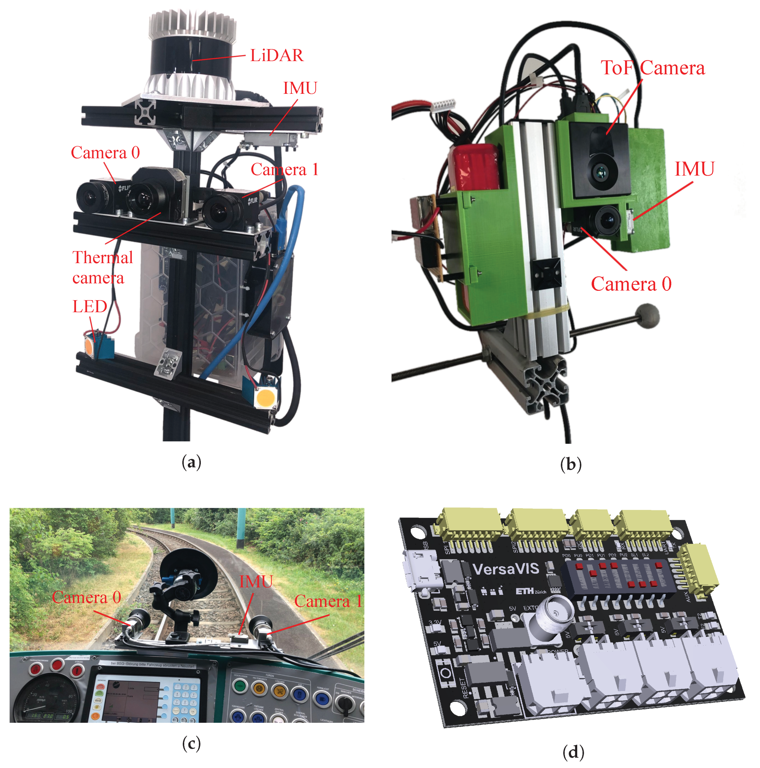
4. Applications
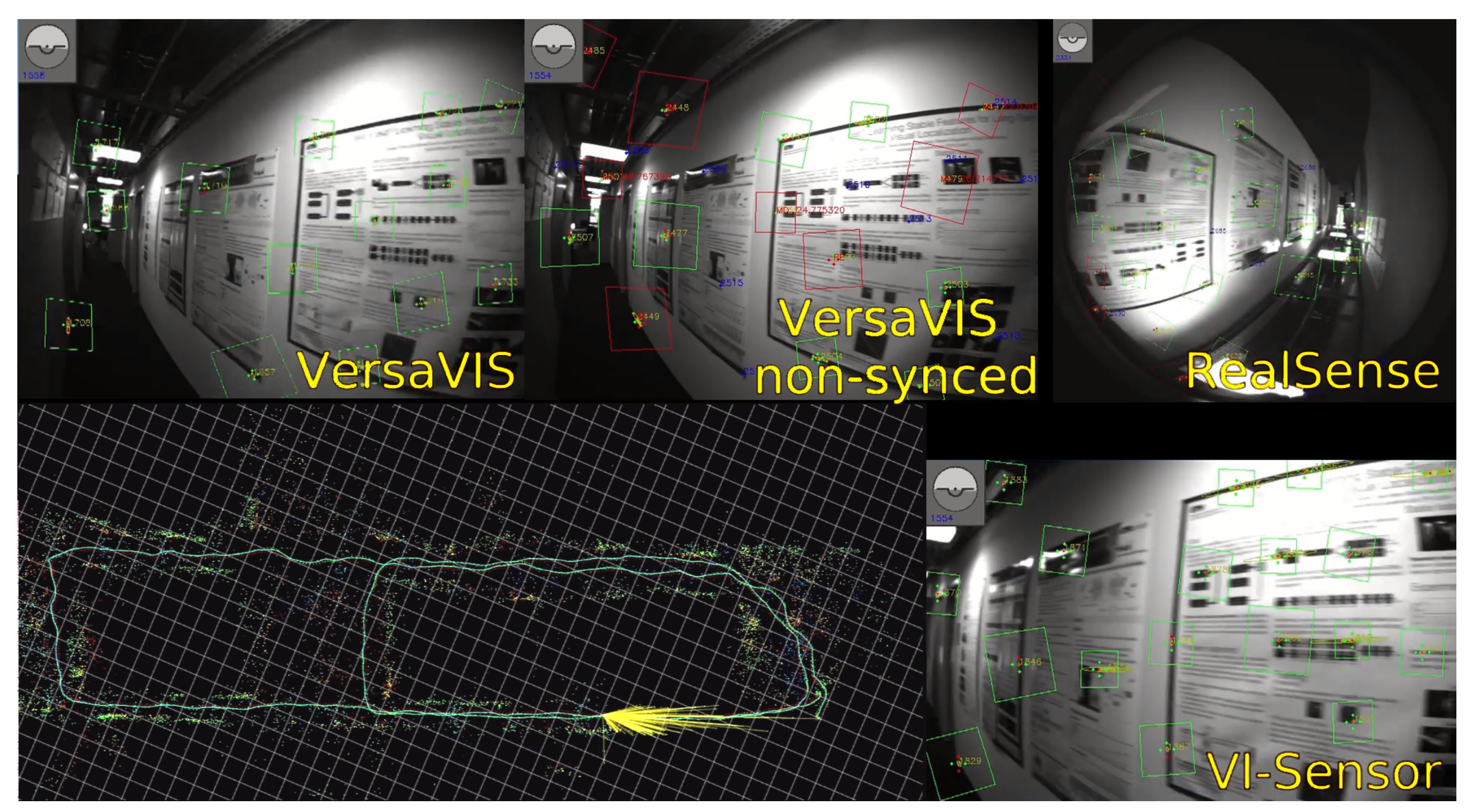
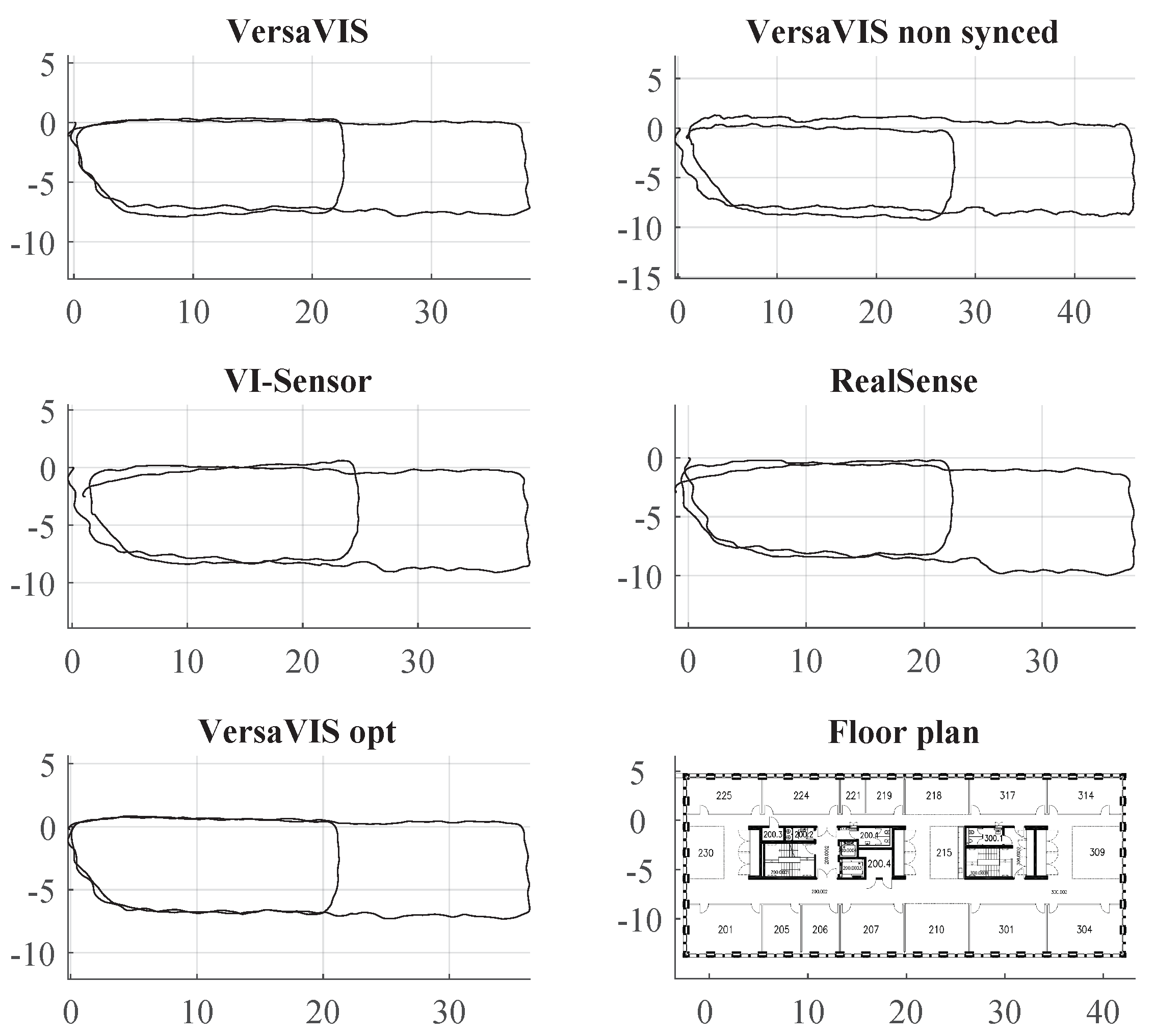
4.1. Visual-Inertial SLAM
4.2. Stereo Visual-Inertial Odometry on Rail Vehicle
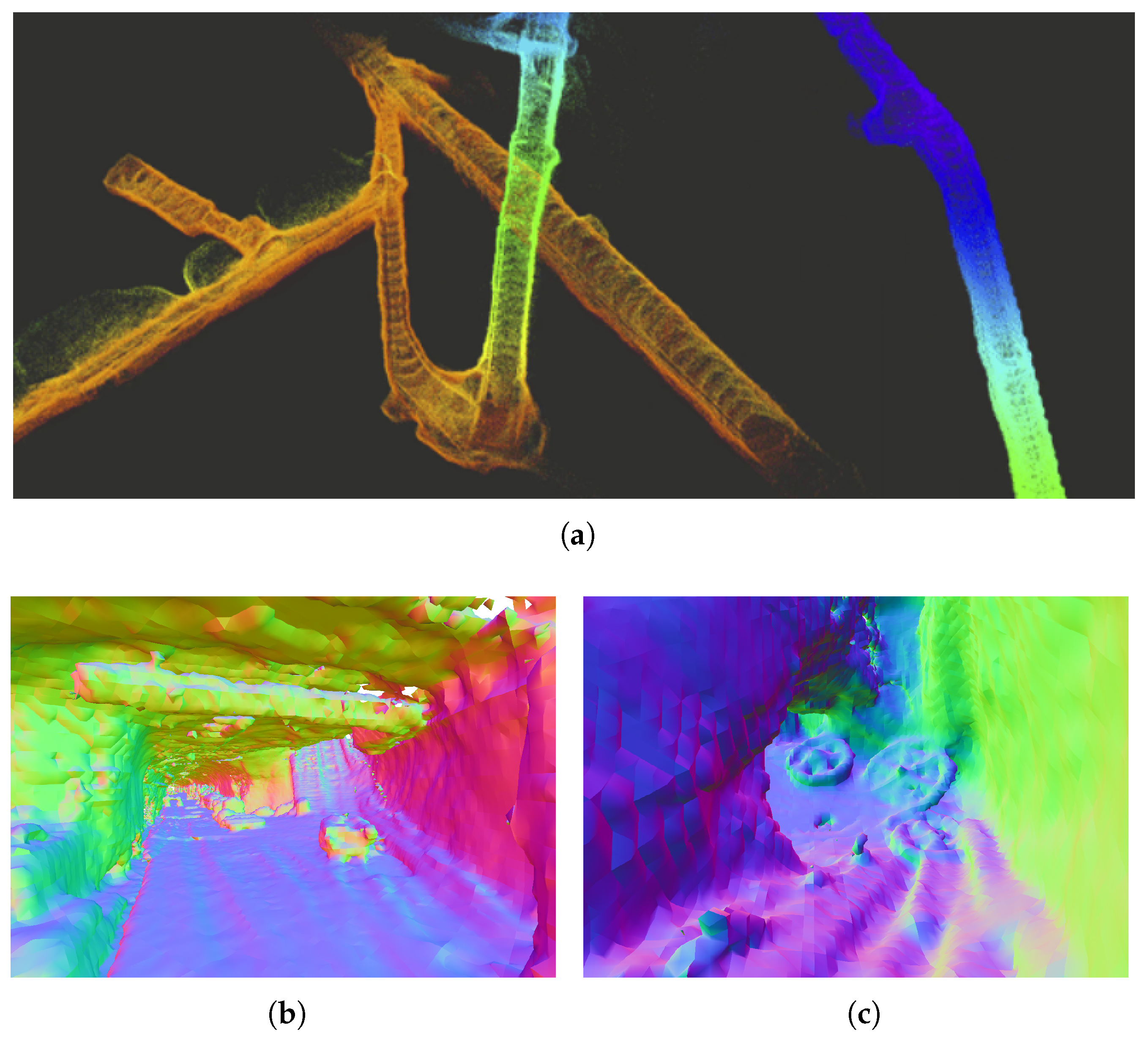
4.3. Multi-Modal Mapping and Reconstruction
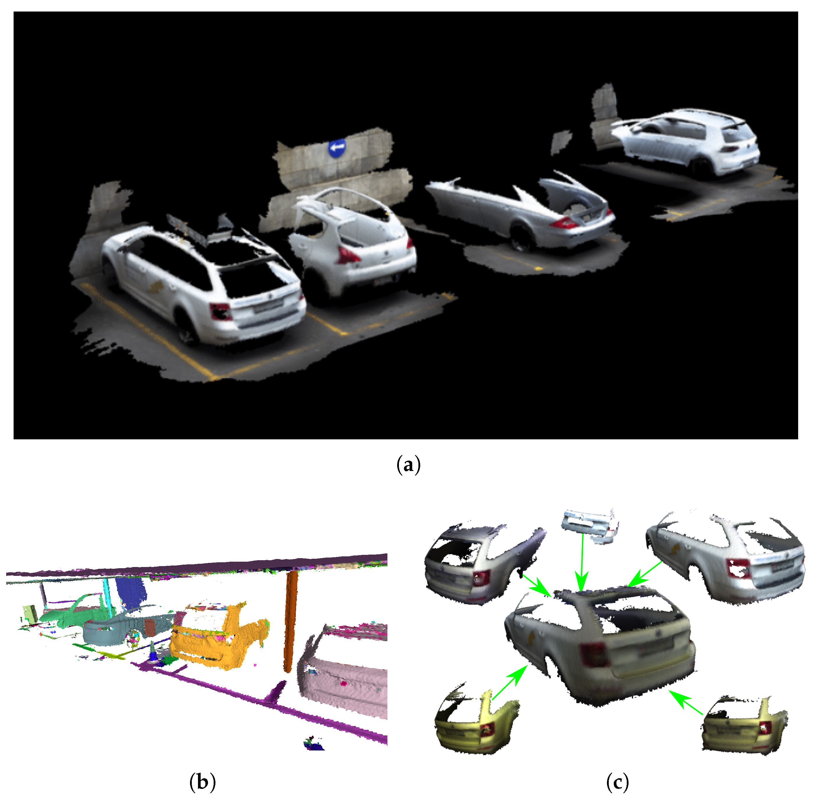
4.4. Object Based Mapping
5. Conclusions
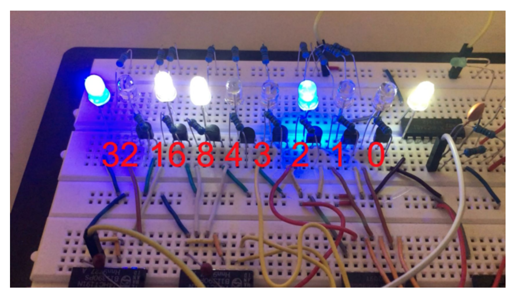
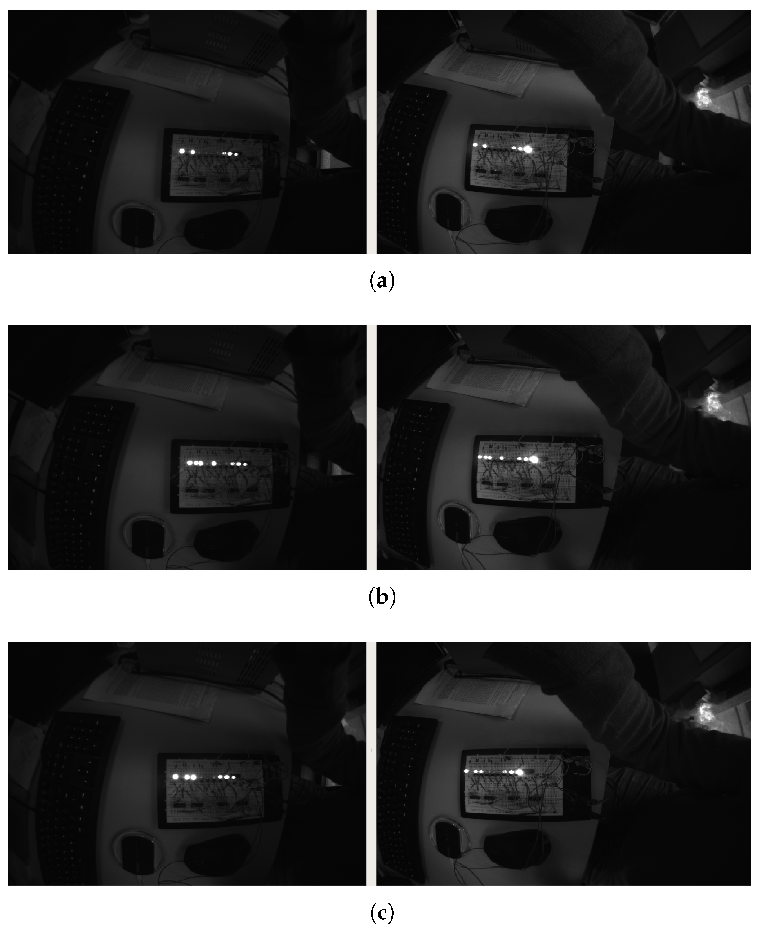
- Illumination module: The VersaVIS triggering board can be paired with LEDs shown in Figure 1a which are triggered corresponding to the longest exposure time of the connected cameras. Thanks to the synchronization, the LEDs can be operated at a higher brightness as which would be possible in continuous operation.
- IMU output: The SPI output of the board enables to use the same IMU which is used in the VI setup for a low-level controller such as the PixHawk [33] used in MAV control.
- Pulse per second (PPS) sync: Some sensors such as specific LiDARs allow synchronization to a PPS signal provided by for example, a Global Position System (GPS) receiver or real-time clock. Using the external clock input on the triggering board, VersaVIS can be extended to synchronize to the PPS source.
- LiDAR synchronization: The available auxiliary interface on VersaVIS could be used to tightly integrate LiDAR measurements by getting digital pulses from the LiDAR corresponding to taken measurements. The merging procedure would then be similar to the one described in Section 2.2.1 for cameras with fixed exposure time.
Author Contributions
Funding
Acknowledgments
Conflicts of Interest
References
- Siegwart, R.; Nourbakhsh, I.R.; Scaramuzza, D. Introduction to Autonomous Mobile Robots, 2nd ed.; MIT Press: Camebridge, MA, USA, 2011; p. 472. [Google Scholar]
- Bloesch, M.; Omari, S.; Hutter, M.; Siegwart, R. Robust visual inertial odometry using a direct EKF-based approach. In Proceedings of the IEEE International Conference on Intelligent Robots and Systems, Hamburg, Germany, 28 September–2 October 2015; pp. 298–304. [Google Scholar] [CrossRef]
- Leutenegger, S.; Lynen, S.; Bosse, M.; Siegwart, R.; Furgale, P. Keyframe-based visual–inertial odometry using nonlinear optimization. Int. J. Robot. Res. 2015, 34, 314–334. [Google Scholar] [CrossRef]
- Qin, T.; Li, P.; Shen, S. VINS-Mono: A Robust and Versatile Monocular Visual-Inertial State Estimator. IEEE Trans. Robot. 2018, 34, 1004–1020. [Google Scholar] [CrossRef]
- Olson, E. A passive solution to the sensor synchronisation problem. In Proceedings of the IEEE/RSJ International Conference on Intelligent Robots and Systems, Taipei, Taiwan, 18–22 October 2010; pp. 1059–1064. [Google Scholar]
- English, A.; Ross, P.; Ball, D.; Upcroft, B.; Corke, P. TriggerSync: A time synchronisation tool. In Proceedings of the IEEE International Conference on Robotics and Automation (ICRA), Seattle, WA, USA, 26–30 May 2015; pp. 6220–6226. [Google Scholar]
- Sommer, H.; Khanna, R.; Gilitschenski, I.; Taylor, Z.; Siegwart, R.; Nieto, J. A low-cost system for high-rate, high-accuracy temporal calibration for LIDARs and cameras. In Proceedings of the IEEE International Conference on Intelligent Robots and Systems, Vancouver, BC, Canada, 24–28 September 2017. [Google Scholar] [CrossRef]
- Lu, L.; Zhang, C.; Liu, Y.; Zhang, W.; Xia, Y. IEEE 1588-based general and precise time synchronization method for multiple sensors*. In Proceeding of the IEEE International Conference on Robotics and Biomimetics, Dali, China, 6–8 December 2019; pp. 2427–2432. [Google Scholar]
- Nikolic, J.; Rehder, J.; Burri, M.; Gohl, P.; Leutenegger, S.; Furgale, P.T.; Siegwart, R. A synchronized visual-inertial sensor system with FPGA pre-processing for accurate real-time SLAM. In Proceeding of the IEEE International Conference on Robotics and Automation, Hong Kong, China, 31 May–7 June 2014; pp. 431–437. [Google Scholar] [CrossRef]
- Burri, M.; Nikolic, J.; Gohl, P.; Schneider, T.; Rehder, J.; Omari, S.; Achtelik, M.W.; Siegwart, R. The EuRoC micro aerial vehicle datasets. Int. J. Robot. Res. 2016, 35, 1157–1163. [Google Scholar] [CrossRef]
- Pfrommer, B.; Sanket, N.; Daniilidis, K.; Cleveland, J. PennCOSYVIO: A challenging visual inertial odometry benchmark. In Proceeding of the IEEE International Conference on Robotics and Automation, Singapore, 29 May–3 June 2017; pp. 3554–3847. [Google Scholar]
- Intel Corporation. Intel® RealSense™ Tracking Camera T265. 2019. Available online: https://www.intelrealsense.com/tracking-camera-t265/ (accessed on 1 February 2020).
- Honegger, D.; Sattler, T.; Pollefeys, M. Embedded real-time multi-baseline stereo. In Proceeding of the IEEE International Conference on Robotics and Automation, Singapore, 29 May–3 June 2017. [Google Scholar]
- Zhang, Z.; Liu, S.; Tsai, G.; Hu, H.; Chu, C.C.; Zheng, F. PIRVS: An Advanced Visual-Inertial SLAM System with Flexible Sensor Fusion and Hardware Co-Design. In Proceeding of the 2018 IEEE International Conference on Robotics and Automation (ICRA), Brisbane, Australia, 21–25 May 2018. [Google Scholar]
- Geiger, A.; Lenz, P.; Stiller, C.; Urtasun, R. Vision meets robotics: The KITTI dataset. Int. J. Robot. Res. 2013, 32, 1231–1237. [Google Scholar] [CrossRef]
- Carlevaris-Bianco, N.; Ushani, A.K.; Eustice, R.M. University of Michigan North Campus long-term vision and lidar dataset. Int. J. Robot. Res. 2016, 35, 1023–1035. [Google Scholar] [CrossRef]
- Majdik, A.L.; Till, C.; Scaramuzza, D. The Zurich urban micro aerial vehicle dataset. Int. J. Robot. Res. 2017, 36. [Google Scholar] [CrossRef]
- Schubert, D.; Goll, T.; Demmel, N.; Usenko, V.; Stückler, J.; Cremers, D. The TUM VI benchmark for evaluating visual-inertial odometry. In Proceeding of the 2018 IEEE/RSJ International Conference on Intelligent Robots and Systems (IROS), Madrid, Spain, 1–5 October 2018. [Google Scholar]
- Arduino Inc. Arduino Zero. 2019. Available online: https://store.arduino.cc/arduino-zero (accessed on 1 February 2020).
- Stanford Artificial Intelligence Laboratory. Robotic Operating System; Stanford Artificial Intelligence Laboratory: Stanford, CA, USA, 2018. [Google Scholar]
- Tschopp, F.; Schneider, T.; Palmer, A.W.; Nourani-Vatani, N.; Cadena Lerma, C.; Siegwart, R.; Nieto, J. Experimental Comparison of Visual-Aided Odometry Methods for Rail Vehicles. IEEE Robot. Autom. Lett. 2019, 4, 1815–1822. [Google Scholar] [CrossRef]
- Furgale, P.; Rehder, J.; Siegwart, R. Unified temporal and spatial calibration for multi-sensor systems. In Proceedings of the IEEE International Conference on Intelligent Robots and Systems, Tokyo, Japan, 3–7 November 2013; pp. 1280–1286. [Google Scholar] [CrossRef]
- Zhang, J.; Singh, S. Visual-lidar odometry and mapping: Low-drift, robust, and fast. In Proceedings of the 2015 IEEE International Conference on Robotics and Automation (ICRA), Seattle, WA, USA, 26–30 May 2015; pp. 2174–2181. [Google Scholar]
- Ferguson, M.; Bouchier, P.; Purvis, M. Rosserial. Available online: http://wiki.ros.org/rosserial (accessed on 1 February 2020).
- Analog Devices. ADIS16448BLMZ: Compact, Precision Ten Degrees of Freedom Inertial Sensor; Technical Report; Analog Devices: Norwood, MA, USA, 2019. [Google Scholar]
- Usenko, V.; Demmel, N.; Cremers, D. The double sphere camera model. In Proceedings of the 2018 International Conference on 3D Vision (3DV), Verona, Italy, 5–8 September 2018; IEEE: Hoboken, NJ, USA, 2018; pp. 552–560. [Google Scholar] [CrossRef]
- Schneider, T.; Dymczyk, M.; Fehr, M.; Egger, K.; Lynen, S.; Gilitschenski, I.; Siegwart, R. maplab: An open framework for research in visual-inertial mapping and localization. IEEE Robot. Autom. Lett. 2018, 3, 1418–1425. [Google Scholar] [CrossRef]
- Nourani-Vatani, N.; Borges, P.V.K. Correlation-based visual odometry for ground vehicles. J. Field Robot. 2011, 28, 742–768. [Google Scholar] [CrossRef]
- Nikolic, J.; Burri, M.; Rehder, J.; Leutenegger, S.; Huerzeler, C.; Siegwart, R. A UAV system for inspection of industrial facilities. In Proceedings of the IEEE Aerospace Conference, Big Sky, MT, USA, 2–9 March 2013. [Google Scholar]
- Oleynikova, H.; Taylor, Z.; Fehr, M.; Siegwart, R.; Nieto, J. Voxblox: Incremental 3D Euclidean Signed Distance Fields for on-board MAV planning. In Proceedings of the IEEE International Conference on Intelligent Robots and Systems, Vancouver, BC, Canada, 24–28 September 2017; pp. 1366–1373. [Google Scholar] [CrossRef]
- Furrer, F.; Novkovic, T.; Fehr, M.; Grinvald, M.; Cadena, C.; Nieto, J.; Siegwart, R. Modelify: An Approach to Incrementally Build 3D Object Models for Map Completion. Int. J. Robot. Res. 2019, submitted. [Google Scholar]
- Furrer, F.; Novkovic, T.; Fehr, M.; Gawel, A.; Grinvald, M.; Sattler, T.; Siegwart, R.; Nieto, J. Incremental Object Database: Building 3D Models from Multiple Partial Observations. In Proceedings of the 2018 IEEE/RSJ International Conference on Intelligent Robots and Systems (IROS), Madrid, Spain, 1–5 October 2018. [Google Scholar]
- Meier, L.; Auterion. Pixhawk 4; Auterion: Zurich, Switzerland, 2019. [Google Scholar]
Sample Availability: Samples of the VersaVIS triggering board are available from the authors. |


| MCU | Hardware Interface | Host Interface | Weight | Size | Price |
|---|---|---|---|---|---|
| ARM M0+ | SPI, IC, UART | Serial-USB 2.0 | <100$ |
| B | N | Reprojection Error | Gyroscope Error | ||||
|---|---|---|---|---|---|---|---|
| Mean | Std | Mean | Std | ||||
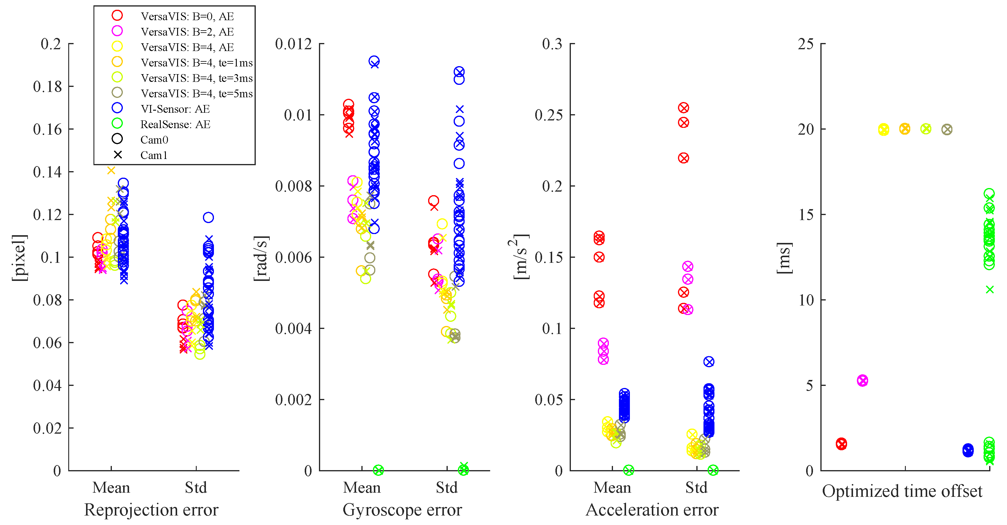
| VersaVIS | 0 | AE | 10 | 0.100078 | 0.064657 | 0.009890 | 0.006353 |
| VersaVIS | 2 | AE | 6 | 0.063781 | 0.007532 | 0.005617 | |
| VersaVIS | 4 | AE | 6 | 0.101866 | 0.067196 | 0.007509 | 0.005676 |
| VersaVIS | 4 | 6 | 0.121552 | 0.075939 | 0.006756 | 0.004681 | |
| VersaVIS | 4 | 6 | 0.108760 | 0.006483 | 0.004360 | ||
| VersaVIS | 4 | 6 | 0.114614 | 0.074536 | 0.006578 | 0.00428 | |
| VI-Sensor | × | AE | 40 | 0.106839 | 0.083605 | 0.008915 | 0.007425 |
| Realsense | × | AE | 40 | 0.436630 | 0.355895 | ||
| N | Accelerometer error | Time offset | |||||
| Mean | Std | Mean | Std | ||||
| VersaVIS | 0 | AE | 10 | 0.143162 | 0.191270 | 1.552360 | 0.034126 |
| VersaVIS | 2 | AE | 6 | 0.083576 | 0.130018 | 5.260927 | 0.035812 |
| VersaVIS | 4 | AE | 6 | 0.030261 | 0.018168 | 19.951467 | 0.049712 |
| VersaVIS | 4 | 6 | 0.026765 | 0.014890 | 20.007137 | 0.047525 | |
| VersaVIS | 4 | 6 | 0.024309 | 0.014367 | 20.002966 | 0.035952 | |
| VersaVIS | 4 | 6 | 0.027468 | 0.016553 | 19.962924 | ||
| VI-Sensor | × | AE | 40 | 0.044845 | 0.042446 | 0.046410 | |
| Realsense | × | AE | 40 | 9.884808 | 5.977421 | ||
| Device | Type | Specification |
|---|---|---|
| Camera | Basler acA1920-155uc | Frame-rate (The hardware is able to capture up to .), Resolution , Dynamic range |
| Lense | Edmund Optics | Focal length opening angle; Aperture |
| IMU | ADIS16445 | Temperature calibrated, , , |
© 2020 by the authors. Licensee MDPI, Basel, Switzerland. This article is an open access article distributed under the terms and conditions of the Creative Commons Attribution (CC BY) license (http://creativecommons.org/licenses/by/4.0/).
Share and Cite
Tschopp, F.; Riner, M.; Fehr, M.; Bernreiter, L.; Furrer, F.; Novkovic, T.; Pfrunder, A.; Cadena, C.; Siegwart, R.; Nieto, J. VersaVIS—An Open Versatile Multi-Camera Visual-Inertial Sensor Suite. Sensors 2020, 20, 1439. https://doi.org/10.3390/s20051439
Tschopp F, Riner M, Fehr M, Bernreiter L, Furrer F, Novkovic T, Pfrunder A, Cadena C, Siegwart R, Nieto J. VersaVIS—An Open Versatile Multi-Camera Visual-Inertial Sensor Suite. Sensors. 2020; 20(5):1439. https://doi.org/10.3390/s20051439
Chicago/Turabian StyleTschopp, Florian, Michael Riner, Marius Fehr, Lukas Bernreiter, Fadri Furrer, Tonci Novkovic, Andreas Pfrunder, Cesar Cadena, Roland Siegwart, and Juan Nieto. 2020. "VersaVIS—An Open Versatile Multi-Camera Visual-Inertial Sensor Suite" Sensors 20, no. 5: 1439. https://doi.org/10.3390/s20051439
APA StyleTschopp, F., Riner, M., Fehr, M., Bernreiter, L., Furrer, F., Novkovic, T., Pfrunder, A., Cadena, C., Siegwart, R., & Nieto, J. (2020). VersaVIS—An Open Versatile Multi-Camera Visual-Inertial Sensor Suite. Sensors, 20(5), 1439. https://doi.org/10.3390/s20051439