Maker Buoy Variants for Water Level Monitoring and Tracking Drifting Objects in Remote Areas of Greenland

 , ,
, , 
Abstract
1. Introduction
2. Materials and Methods
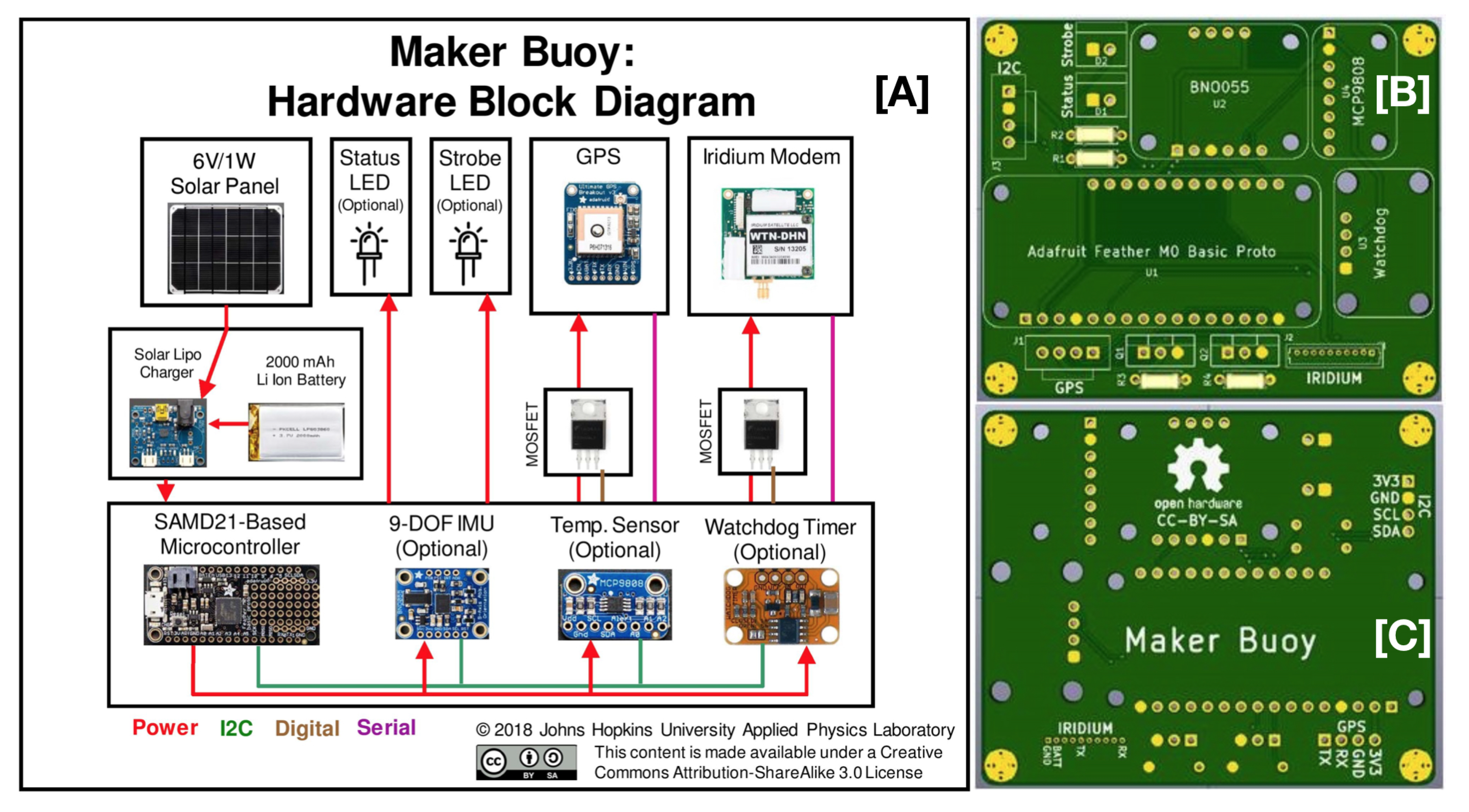
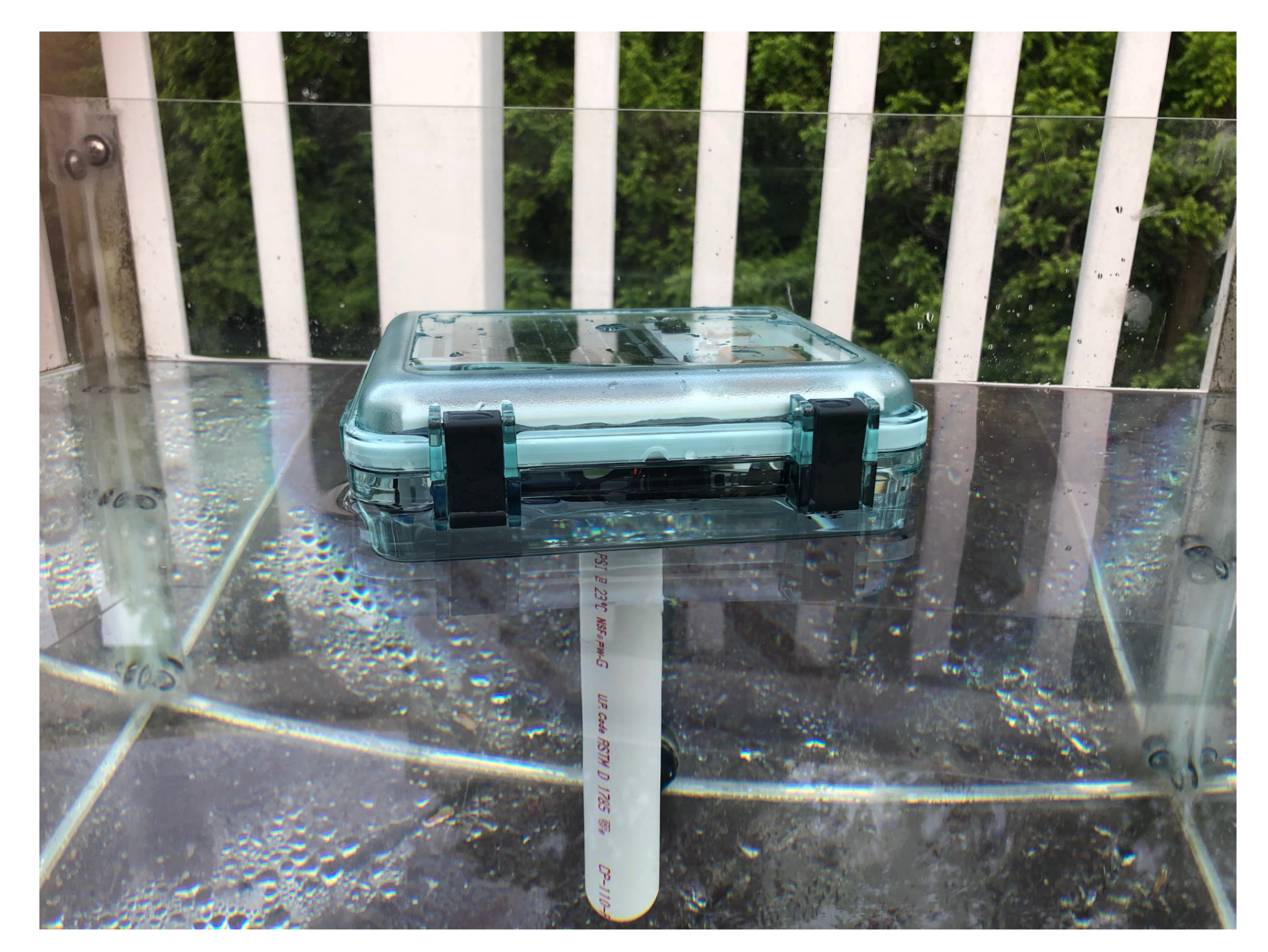
2.1. Maker Buoy Design
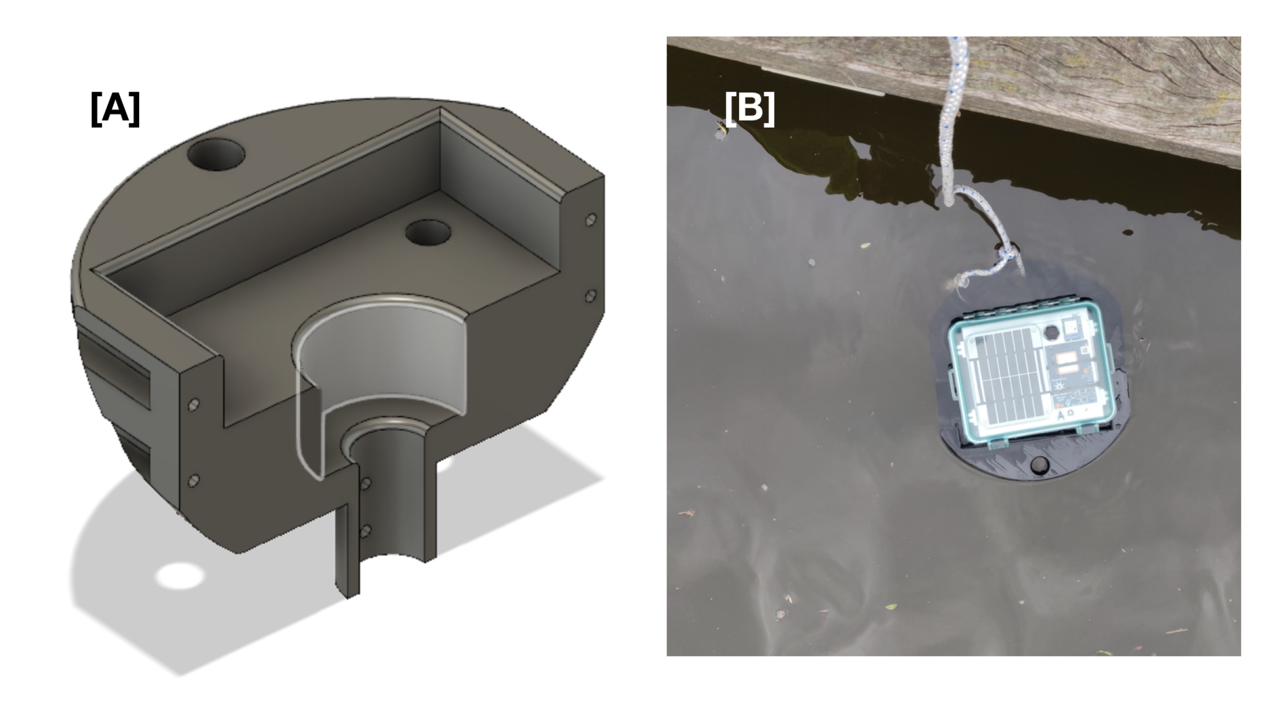
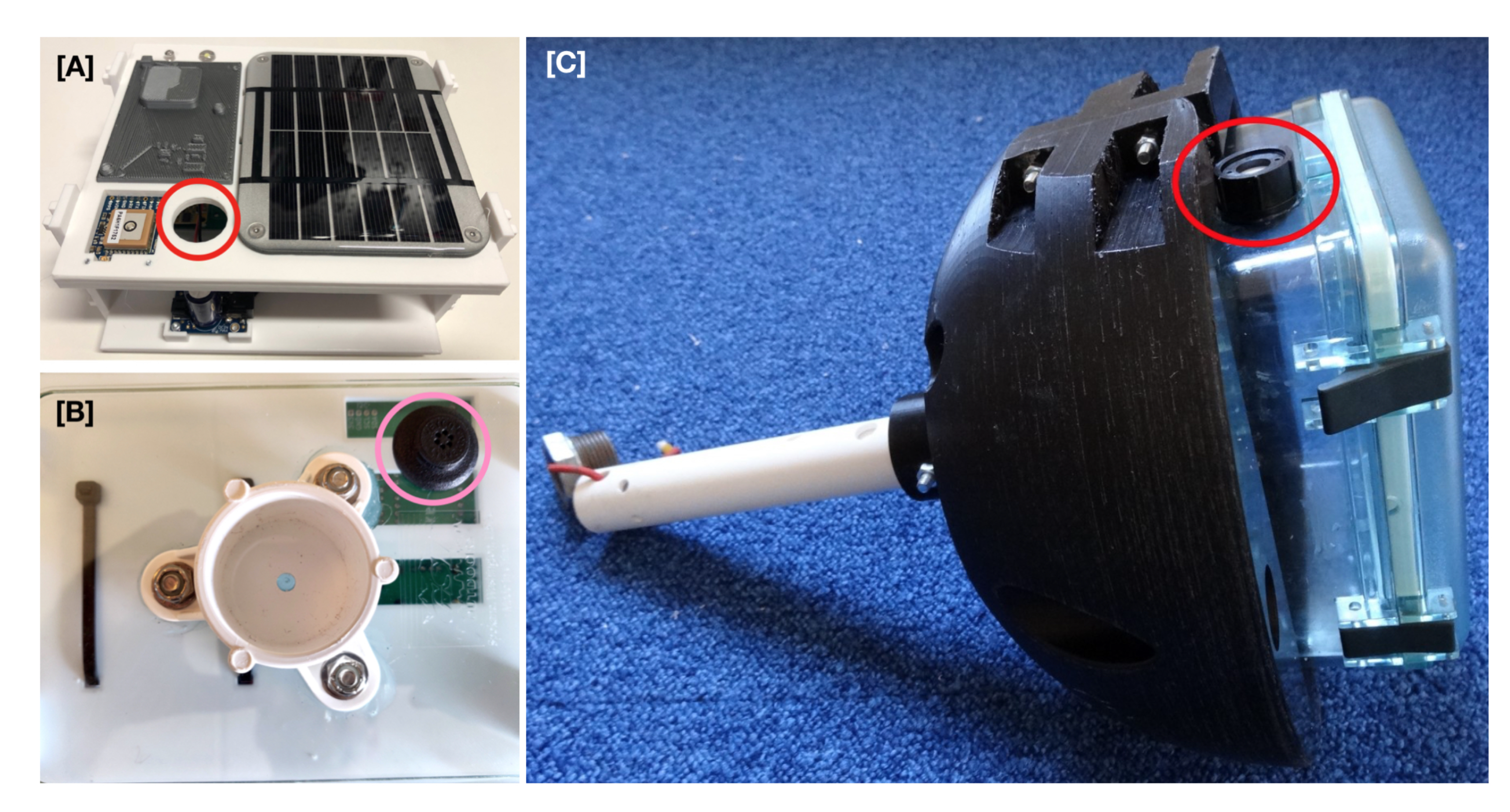
2.2. GLOF Buoy
2.3. Drifting Buoy
2.4. Data Access and Management
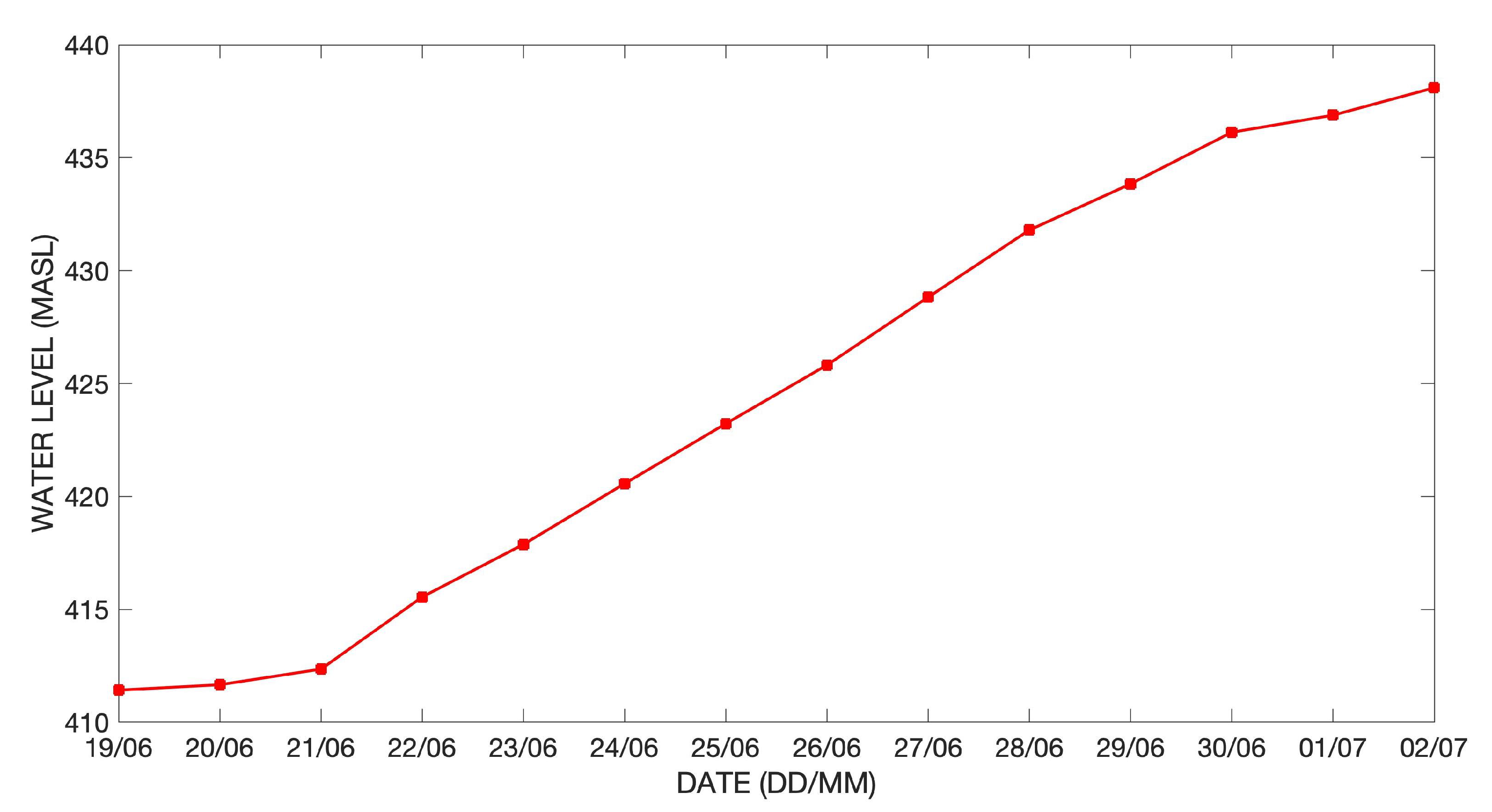
2.5. Hullet Lake
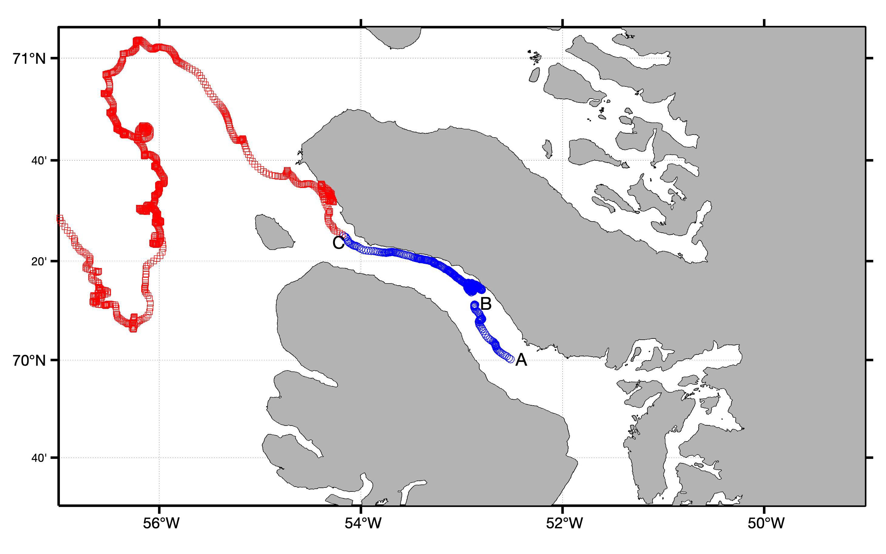
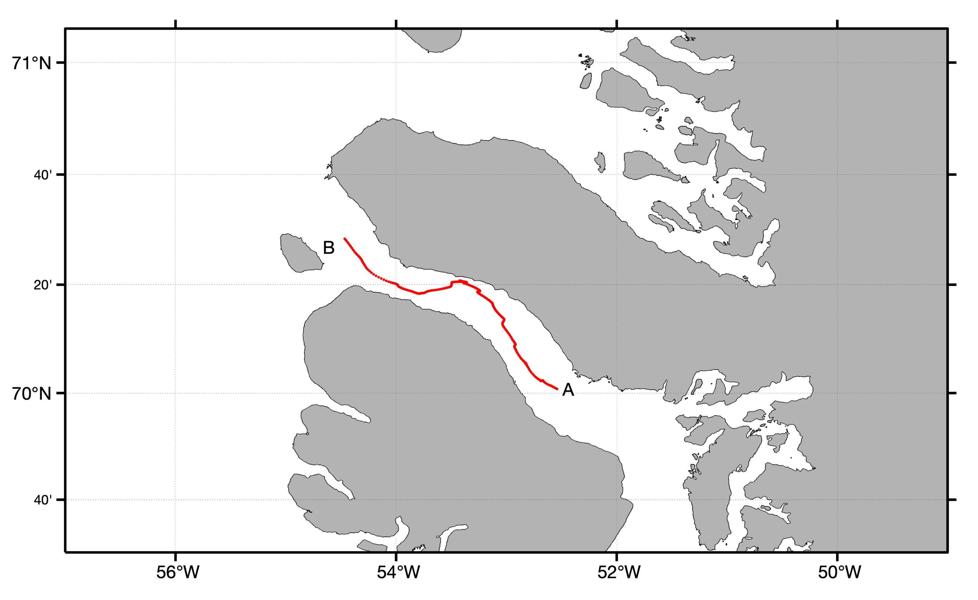
2.6. Vaigat Strait
3. Results and Discussion
3.1. GLOF Buoys
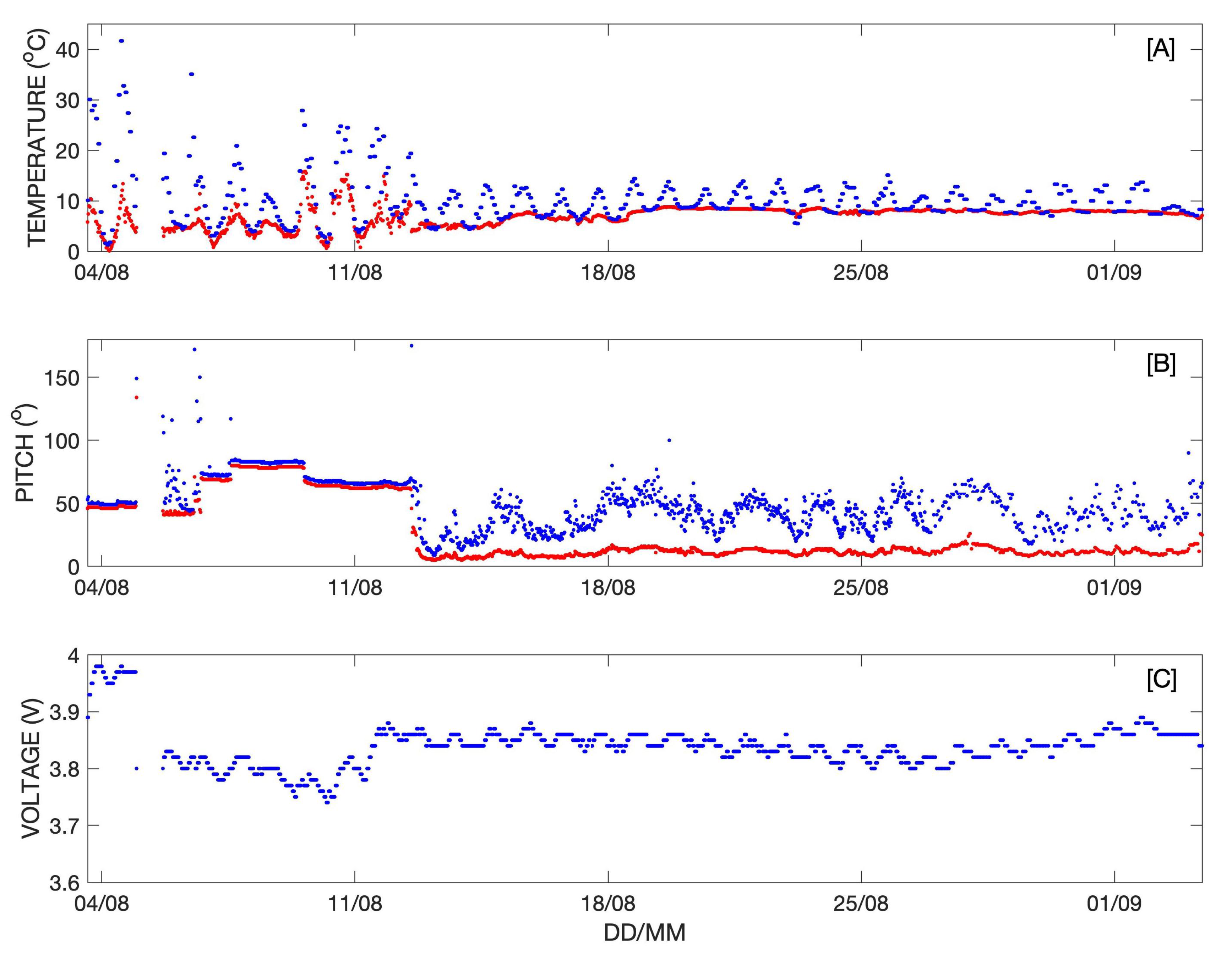
3.2. Drifting Buoys
3.2.1. Iceberg tracking
3.2.2. Drifting Mooring Tracking
4. Summary
Author Contributions
Funding
Acknowledgments
Conflicts of Interest
Abbreviations
| ° | Degrees |
| 3D | Three-dimensional |
| ASCII | American Standard Code for Information Interchange |
| ASL | Above Sea Level |
| BOM | Bill of Materials |
| °C | Degrees Celsius |
| EWS | Early Warning System |
| EXITE | Expendable Ice Tracker |
| FTDI | Future Technology Devices International |
| GLOF | Glacial Lake Outburst Flood |
| GPS | Global Positioning System |
| GrIS | Greenland Ice Sheet |
| hPa | Hecto-Pascal |
| IDE | Integrated Development Environment |
| IMEI | International Mobile Equipment Identity |
| IMU | Inertial Motion Unit |
| km | Kilometer |
| LED | Light Emitting Diode |
| LiPo | Lithium Polymer |
| m | Meter |
| mAh | Milli-amp Hour |
| min | Minute |
| PCB | Printed Circuit Board |
| PETG | Polyethylene Terephthalate Glycol |
| PVC | Polyvinyl Chloride |
| RTK | Real-Time Kinematic |
| SBD | Short-Burst Data |
| SfM | Structure from Motion |
| SMA | SubMiniature version A |
| SST | Sea Surface Temperature |
| SWAP | Size, Weight, and Power |
| TTL | Transistor-Transistor Logic |
| USB | Universal Serial Bus |
| V | Volts |
| VIMOA | Vaigat Iceberg Microbial Oil degradation and Archaeological heritage investigation |
Appendix A. Field Data Access


- Click on the ‘port’ tab
- On the ‘Port’ drop-down menu - select \VCP0
- Select 19200 baud rate
- Click ‘open’ twice
- Click on the ‘send’ tab
- In the top left dialogue box enter the following commands, followed by ‘Send ASCII’
- Check modem communication: AT\r
- –
- Response: OK\r
- Turn off Flow Control: AT\&K0
- –
- Response: OK\r
- Start short burst data (SBD) session: AT+SBDIX\r
- –
- Response format: +SBDIX: transmit status, message number (TX), message status, message number (RX), message length, number of queued messages
- –
- transmit status: A value between 0-2 indicates that your AT+SBDIX\r message was received while any number >2 indicates that your message was not received.
- –
- message number (TX): The number of the message (AT+SBDIX\r), which can be ignored
- –
- message status: A number between 0-2
- ∗
- 0: No messages waiting
- ∗
- 1: New message retrieved
- ∗
- 2: Error
- –
- message number (RX): Number of the message received, which can be ignored
- –
- message length: Length of the message, in bytes
- –
- number of queued messages: self-explanatory
- If your message was not received (transmit status >2), make sure that the antenna has an unimpeded view to the sky and send AT+SBDIX\r again
- If transmit status is between 0-2, navigate to the ‘Capture’ tab in RealTerm
- Enter the desired directory and file name in the file dialogue box
- Check the box that reads ‘Capture as Hex’
- Click either ‘Start: Overwrite’ or ‘Start: Append’
- Navigate to the ‘Send’ tab in RealTerm
- Enter AT+SBDRB\r and click ‘Send ASCII’
- Navigate to the ‘Capture’ tab in RealTerm and click ‘Stop Capture’
- Open the file that was created from your RealTerm session and verify the contents. Note that the first 11 HEX characters in the capture file correspond to AT+SBDRB<CR> followed by a two-byte HEX containing the message length
- Download any additional messages by repeating this process
- Once finished, navigate to the ‘Port’ tab in RealTerm and click on ‘Open’ to close the port
- Open RealTerm and connect to the field RockBlock by following the instructions above
- Send the following commands, followed by ‘Send ASCII’
- –
- AT\r
- –
- AT\&K0
- –
- AT+SBDIX\r
- –
- AT+SBDWT=FLUSH_MT\r
- –
- AT+SBDIX\r
References
- Ahlstrøm, A.; Petersen, D.; Langen, P.; Citterio, M.; Box, J. Abrupt shift in the observed runoff from the southwestern Greenland Ice Sheet. Sci. Adv. 2017, 3, e1701169. [Google Scholar] [CrossRef] [PubMed]
- Bevis, M.; Harig, C.; Khan, S.A.; Brown, A.; Simons, F.J.; Willis, M.; Fettweis, X.; van den Broeke, M.R.; Madsen, F.B.; Kendrick, E.; et al. Accelerating changes in ice mass within Greenland, and the ice sheet’s sensitivity to atmospheric forcing. Proc. Natl. Acad. Sci. USA 2019, 116, 1934–1939. [Google Scholar] [CrossRef] [PubMed]
- Bian, Y.; Yue, J.; Gao, W.; Li, Z.; Lu, D.; Xiang, Y.; Chen, J. Analysis of the spatiotemporal changes of ice sheet mass and driving factors in Greenland. Remote Sens. 2019, 11, 862. [Google Scholar] [CrossRef]
- Ryan, J.; Smith, L.; van As, D.; Cooley, S.; Cooper, M.; Pitcher, L.; Hubbard, A. Greenland Ice Sheet surface melt amplified by snowline migration and bare ice exposure. Sci. Adv. 2019, 5, eaav3738. [Google Scholar] [CrossRef]
- Chen, X.; Zhang, X.; Church, J.A.; Watson, C.S.; King, M.A.; Monselesan, D.; Legresy, B.; Harig, C. The increasing rate of global mean sea-level rise during 1993–2014. Nat. Clim. Change 2017, 7, 492–495. [Google Scholar] [CrossRef]
- Sejr, M.; Stedmon, C.; Bendtsen, J.; Abermann, J.; Juul-Pedersen, T.; Mortensen, J.; Rysgaard, S. Evidence of local and regional freshening of Northeast Greenland coastal waters. Sci. Rep. 2017, 7, 13183. [Google Scholar] [CrossRef]
- Boone, W.; Rysgaard, S.; Carlson, D.; Meire, L.; Kirillov, S.; Mortensen, J.; Dmitrenko, I.; Vergeynst, L.; Sejr, M. Coastal freshening prevents fjord bottom water renewal in Northeast Greenland: A mooring study from 2003 to 2015. Geophys. Res. Lett. 2018, 45, 2726–2733. [Google Scholar] [CrossRef]
- Dawson, A. Glacier-dammed lake investigations in the Hullet Lake area, South Greenland. Medd. Groenl.: Geosc. 1983, 11, 24. [Google Scholar]
- Russell, A. A comparison of two recent Jökulhlaups from an ice-dammed lake, Søndre Strømfjord, West Greenland. J. Glaciol. 1989, 35, 157–162. [Google Scholar] [CrossRef][Green Version]
- Fukui, H.; Limlahapun, P.; Kameoka, T. Real time Monitoring for Imja Glacial Lake in Himalaya—Global Warming Front Monitoring System. In Proceedings of the SICE Annual Conference 2008, Tokyo, Japan, 20–22 August 2008. [Google Scholar] [CrossRef]
- Petrakov, D.; Tutubalina, O.; Aleinikov, A.; Chernomorets, S.; Evans, S.; Kidyaeva, V.; Krylenko, I.N.; Norin, S.; Shakhmina, M.; Seynova, I. Monitoring of Bashkara Glacier lakes (Central Caucasus, Russia) and modelling of their potential outburst. Nat. Hazards 2011, 61, 1293–1316. [Google Scholar] [CrossRef]
- Jain, S.K.; Lohani, A.K.; Singh, R.; Chaudhary, A.; Thakural, L. Glacial lakes and glacial lake outburst flood in a Himalayan basin using remote sensing and GIS. Nat. Hazards 2012, 62, 887–899. [Google Scholar] [CrossRef]
- Emmer, A.; Vilímek, V.; Huggel, C.; Klimeš, J.; Schaub, Y. Limits and challenges to compiling and developing a database of glacial lake outburst floods. Landslides 2016, 13, 1579–1584. [Google Scholar] [CrossRef]
- Emmer, A. GLOFs in the WOS: bibliometrics, geographies and global trends of research on glacial lake outburst floods (Web of Science, 1979–2016). Nat. Hazards Earth Syst. Sci. 2018, 18, 813–827. [Google Scholar] [CrossRef]
- Narama, C.; Duishonakunov, M.; Kääb, A.; Daiyrov, M.; Abdrakhmatov, K. The 24 July 2008 outburst flood at the western Zyndan glacier lake and recent regional changes in glacier lakes of the Teskey Ala-Too range, Tien Shan, Kyrgyzstan. Nat. Hazards Earth Syst. Sci. 2010, 10, 647–659. [Google Scholar] [CrossRef]
- Koschitzki, R.; Schwalbe, E.; Maas, H.G. An autonomous image based approach for detecting glacial lake outburst floods. In Proceedings of the International Archives of the Photogrammetry, Remote Sensing and Spatial Information Sciences, Riva del Garda, Italy, 23–25 June 2014; Volume 45, pp. 337–342. [Google Scholar] [CrossRef]
- Kjeldsen, K.; Mortensen, J.; Bendtsen, J.; Petersen, D.; Lennert, K.; Rysgaard, S. Ice-dammed lake drainage cools and raises surface salinities in a tidewater outlet glacier fjord, west Greenland. J. Geophys. Res. Earth Surf. 2014, 119, 1310–1321. [Google Scholar] [CrossRef]
- Ross, L.; Pérez-Santos, I.; Parady, B.; Castro, L.; Valle-Levinson, A.; Schneider, W. Glacial Lake Outburst Flood (GLOF) Events and Water Response in A Patagonian Fjord. Water 2020, 12, 248. [Google Scholar] [CrossRef]
- Zhang, G.; Yao, T.; Xie, H.; Wang, W.; Yang, W. An inventory of glacial lakes in the Third Pole region and their changes in response to global warming. Global Planet. Change 2015, 131, 148–157. [Google Scholar] [CrossRef]
- Rounce, D.R.; Watson, C.S.; McKinney, D.C. Identification of Hazard and Risk for Glacial Lakes in the Nepal Himalaya Using Satellite Imagery from 2000–2015. Remote Sens. 2017, 9, 654. [Google Scholar] [CrossRef]
- Arp, C.; Jones, B.; Whitman, M.; Larsen, A.; Urban, F. Lake temperature and ice cover regimes in the Alaskan subarctic and arctic: Integrated monitoring, remote sensing, and modeling. J. Am. Water Resour. Assoc. 2010, 46, 777–791. [Google Scholar] [CrossRef]
- Sulak, D.; Sutherland, D.; Enderlin, E.; Stearns, L.; Hamilton, G. Iceberg properties and distributions in three Greenlandic fjords using satellite imagery. Ann. Glaciol. 2017, 58, 92–106. [Google Scholar] [CrossRef]
- Flowers, G. Hydrology and the future of the Greenland Ice Sheet. Nat. Commun. 2018, 9, 2729. [Google Scholar] [CrossRef] [PubMed]
- Hopwood, M.; Carroll, D.; Höfer, J.; Achterberg, E.; Meire, L.; LeMoigne, F.; Bach, L.; Eich, C.; Sutherland, D.; Gonzalez, H. Highly variable iron content modulates iceberg-ocean fertilisation and potential carbon export. Nat. Commun. 2019, 10, 5261. [Google Scholar] [CrossRef] [PubMed]
- Turbull, I.; Fournier, N.; Stolwijk, M.; Fosnaes, T.; McGonical, D. Operational iceberg drift forecasting in Northwest Greenland. Cold Reg. Sci. Technol. 2015, 110, 1–18. [Google Scholar] [CrossRef]
- Kim, E.; Utne, I.; Kim, H. Applying CAST to investigation of the FPSO’s incident with an iceberg. In Proceedings of the 25th International Conference on Port and Ocean Engineering under Arctic Conditions, Delft, The Netherlands, 9–13 June 2019. [Google Scholar]
- Carlson, D.; Boone, W.; Meire, L.; Abermann, J.; Rysgaard, S. Bergy Bit and Melt Water Trajectories in Godthåbsfjord (SW Greenland) Observed by the Expendable Ice Tracker. Front. Mar. Sci. 2017, 4, 276. [Google Scholar] [CrossRef]
- Carlson, D.; Rysgaard, S. Adapting open-source drone autopilots for real-time iceberg observations. MethodsX 2018, 5, 1059–1072. [Google Scholar] [CrossRef] [PubMed]
- Enderlin, E.M.; Carrigan, C.J.; Kochtitzky, W.H.; Cuadros, A.; Moon, T.; Hamilton, G.S. Greenland iceberg melt variability from high-resolution satellite observations. Cryosphere 2018, 12, 565–575. [Google Scholar] [CrossRef]
- MacAyeal, D.; Abbot, D.; Sergienko, O. Iceberg-capsize tsunamigenesis. Ann. Glaciol. 2011, 52, 51–56. [Google Scholar] [CrossRef]
- Carlson, D. 3D printed protective sleeve for the Maker Buoy Glacial Lake Water Level Monitoring Buoy. Available online: https://data.mendeley.com/datasets/vn69vmdbvj/1 (accessed on 9 December 2019).
- Weidick, A. Ice margin features in the Julianehab district, South Greenland. Medd. Groenl. 1963, 163, 133. [Google Scholar]
- Clement, P. Observationer Omkring Hullet—en Isdæmmet sø i Sydgrønland. Available online: https://2dgf.dk/xpdf/dgfaars1983-65-71.pdf (accessed on 22 February 2020).
- Honda, K.; Shrestha, A.; Witayangkurn, A.; Chinnachodteeranun, R.; Shimamura, H. Fieldservers and Sensor Service Grid as Real-time Monitoring Infrastructure for Ubiquitous Sensor Networks. Sensors 2009, 9, 2363–2370. [Google Scholar] [CrossRef]
- Kirkham, J.; Rosser, N.; Wainwright, J.; Vann Jones, E.; Dunning, S.; Lane, V.; Hawthorn, D.; Strzelecki, M.; Szczuciński, W. Drift-dependent changes in iceberg size-frequency distributions. Sci. Rep. 2017, 7, 15991. [Google Scholar] [CrossRef]
- Mascarenhas, V.; Zielinski, O. Hydrography-Driven Optical Domains in the Vaigat-Disko Bay and Godthabsfjord: Effects of Glacial Meltwater Discharge. Front. Mar. Sci. 2019, 6, 335. [Google Scholar] [CrossRef]
- Bojesen-Koefoed, J.; Bidstrup, T.; Christiansen, F.; Dalhoff, F.; Gregersen, U.; Nytoft, H.; Nøhr-Hansen, H.; Pedersen, A.; Sønderholm, M. Petroleum seepages at Asuk, Disko, West Greenland: Implications for regional petroleum exploration. J. Pet. Geol 2007, 30, 219–236. [Google Scholar] [CrossRef]
- Walsh, M.; Tejsner, P.; Carlson, D.; Vergeynst, L.; Kjeldsen, K.; Gründiger, F.; Dai, H.; Thomsen, S.; Larsen, E. The VIMOA project and archaeological heritage in the Nuussuaq Peninsula, northwest Greenland. Antiquity 2020, 94, e6. [Google Scholar] [CrossRef]
- Carlson, D.; Pasma, J.; Jacobsen, M.; Hansen, M.; Thomsen, S.; Lillethorup, J.; Tirsgaard, F.; Flytkjær, A.; Melvad, C.; Laufer, K.; et al. Retrieval of ice samples using the Ice Drone. Front. Earth Sci. 2019, 7, 287. [Google Scholar] [CrossRef]
- Thomsen, S.; Tirsgaard, F.; Hansen, M.; Lillethorup, J.; Flytkær, A.; Carlson, D.; Melvad, C.; Rysgaard, S. An affordable and miniature ice coring drill for rapid acquisition of small iceberg samples. HardwareX 2020. In Press. [Google Scholar] [CrossRef]
- Crawford, A.; Mueller, D.; Joyal, G. Surveying Drifting Icebergs and Ice Islands: Deterioration Detection and Mass Estimation with Aerial Photogrammetry and Laser Scanning. Remote Sens. 2018, 10, 575. [Google Scholar] [CrossRef]
- Vergeynst, L.; Christensen, J.; Kjeldsen, K.; Meire, L.; Boone, W.; Malmquist, L.; Rysgaard, S. In situ biodegradation, photooxidation and dissolution of petroleum compounds in Arctic seawater and sea ice. Water Res. 2018, 148, 459–468. [Google Scholar] [CrossRef]
- Neumann, T.; Martino, A.; Markus, T.; Bae, S.; Bock, M.; Brenner, A.; Brunt, K.; Cavanaugh, J.; Fernandes, S.; Hancock, D.; et al. The Ice, Cloud, and Land Elevation Satellite – 2 mission: A global geolocated photon product derived from the Advanced Topographic Laser Altimeter System. Remote Sens. Environ. 2019, 233, 111325. [Google Scholar] [CrossRef]
- Zhang, G.; Chen, W.; Xie, H. Tibetan Plateau’s Lake Level and Volume Changes From NASA’s ICESat/ICESat-2 and Landsat Missions. Geophys. Res. Lett. 2019, 46, 13107–13118. [Google Scholar] [CrossRef]


© 2020 by the authors. Licensee MDPI, Basel, Switzerland. This article is an open access article distributed under the terms and conditions of the Creative Commons Attribution (CC BY) license (http://creativecommons.org/licenses/by/4.0/).
Share and Cite
Carlson, D.F.; Pavalko, W.J.; Petersen, D.; Olsen, M.; Hass, A.E. Maker Buoy Variants for Water Level Monitoring and Tracking Drifting Objects in Remote Areas of Greenland. Sensors 2020, 20, 1254. https://doi.org/10.3390/s20051254
Carlson DF, Pavalko WJ, Petersen D, Olsen M, Hass AE. Maker Buoy Variants for Water Level Monitoring and Tracking Drifting Objects in Remote Areas of Greenland. Sensors. 2020; 20(5):1254. https://doi.org/10.3390/s20051254
Chicago/Turabian StyleCarlson, Daniel F., Wayne J. Pavalko, Dorthe Petersen, Martin Olsen, and Andreas E. Hass. 2020. "Maker Buoy Variants for Water Level Monitoring and Tracking Drifting Objects in Remote Areas of Greenland" Sensors 20, no. 5: 1254. https://doi.org/10.3390/s20051254
APA StyleCarlson, D. F., Pavalko, W. J., Petersen, D., Olsen, M., & Hass, A. E. (2020). Maker Buoy Variants for Water Level Monitoring and Tracking Drifting Objects in Remote Areas of Greenland. Sensors, 20(5), 1254. https://doi.org/10.3390/s20051254