A New Edge Patch with Rotation Invariance for Object Detection and Pose Estimation


Abstract
1. Introduction
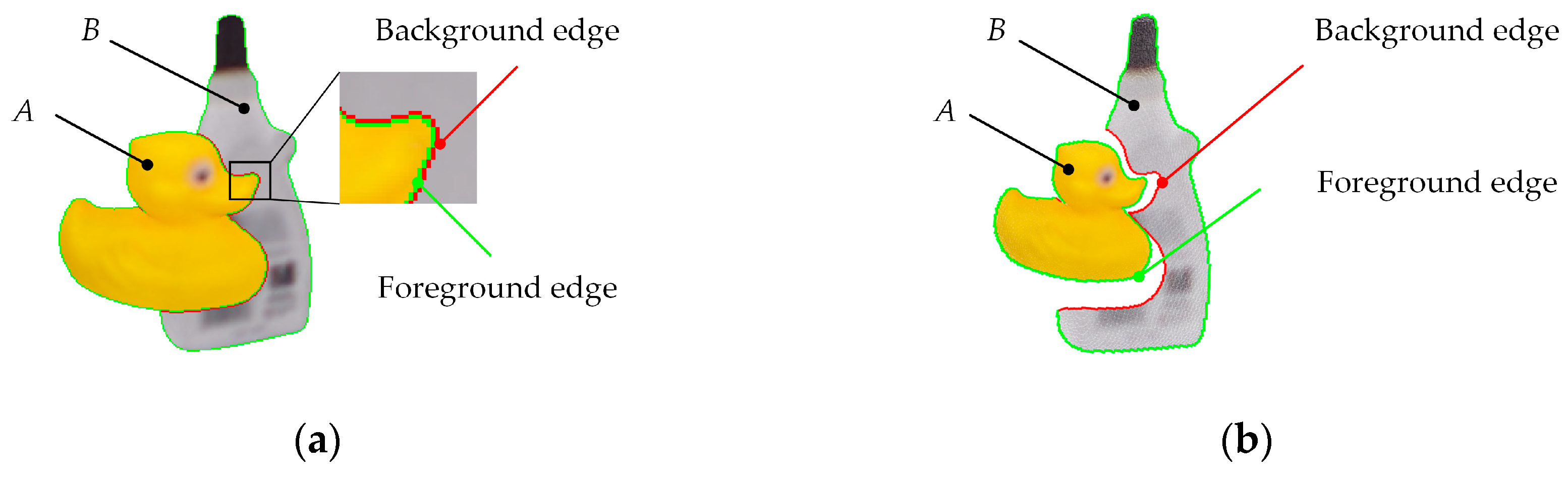
- The E-patch is rotation invariant. In the sampling process, a canonical orientation is extracted to make the E-patch rotation invariant. Thus, it is not necessary to expand the E-patch library by rotating rendering views of the target object, avoiding quantization errors in the process of feature matching.
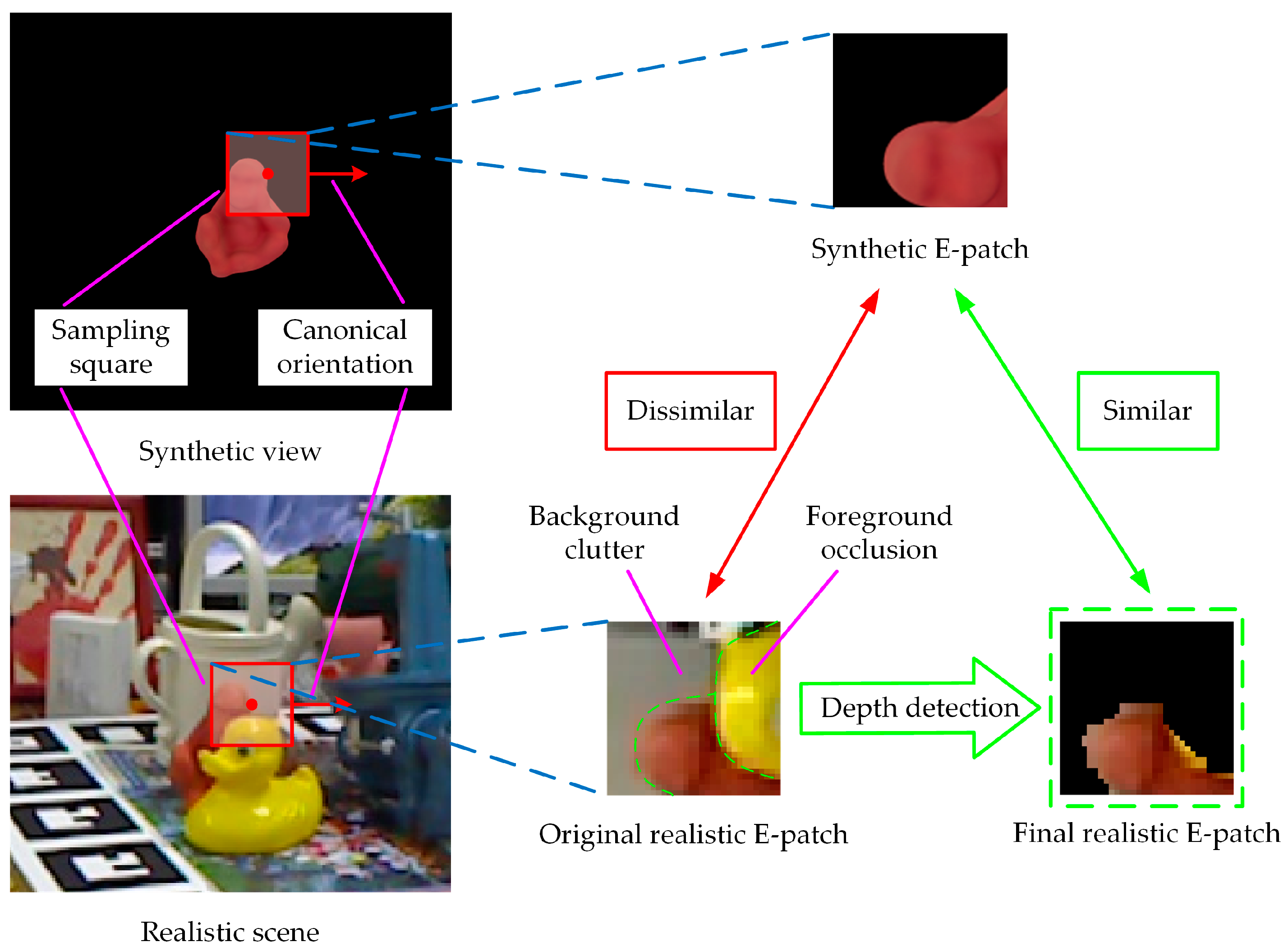
- The E-patch contains less scene interference. During the depth detection process, the scene interference is eliminated in the four channels of E-patch. This ensures the robustness of the E-patch against scene interference.
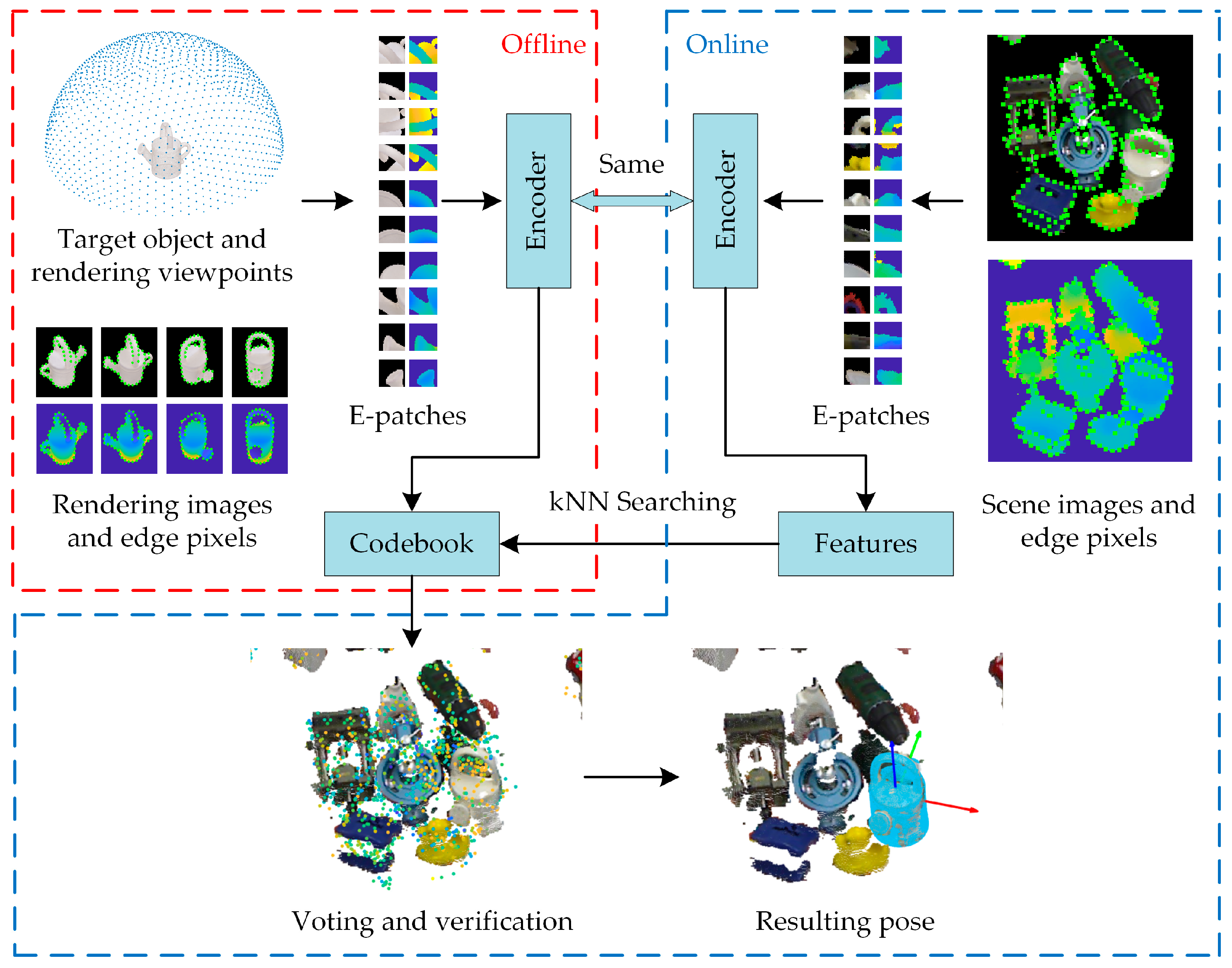
2. Methods
2.1. E-Patch Generation
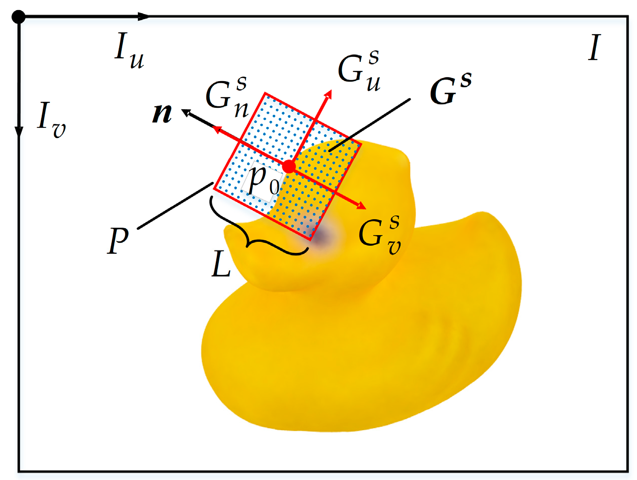
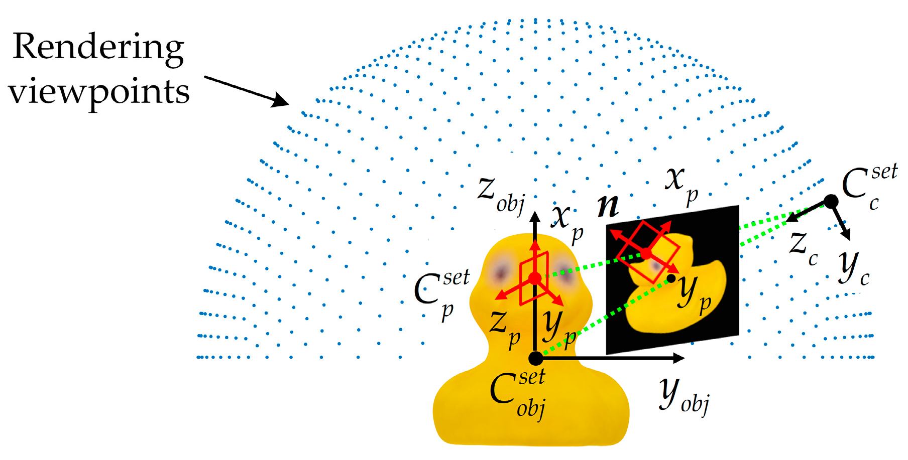
2.1.1. Sampling Center Extraction
2.1.2. E-Patch Sampling along a Canonical Orientation
2.1.3. Depth Detection
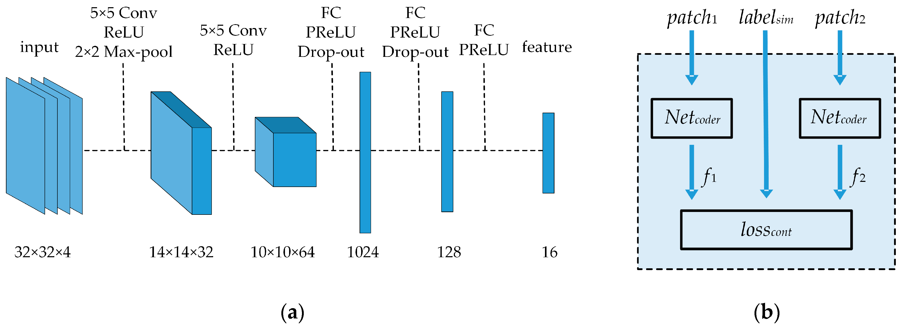
2.2. Encoding Network Training
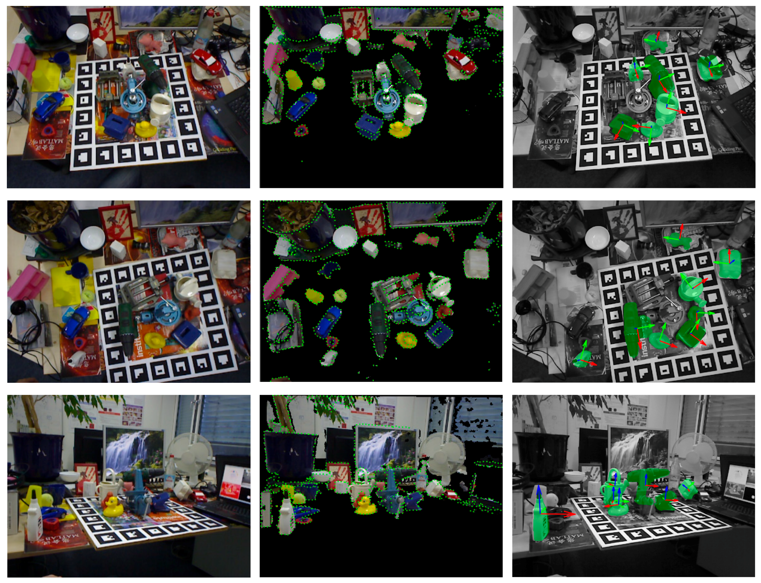
2.3. Object Detection and Pose Estimation Based on E-patch
2.3.1. Offline Construction of the Codebook
2.3.2. Online Testing
3. Experiments and Discussion
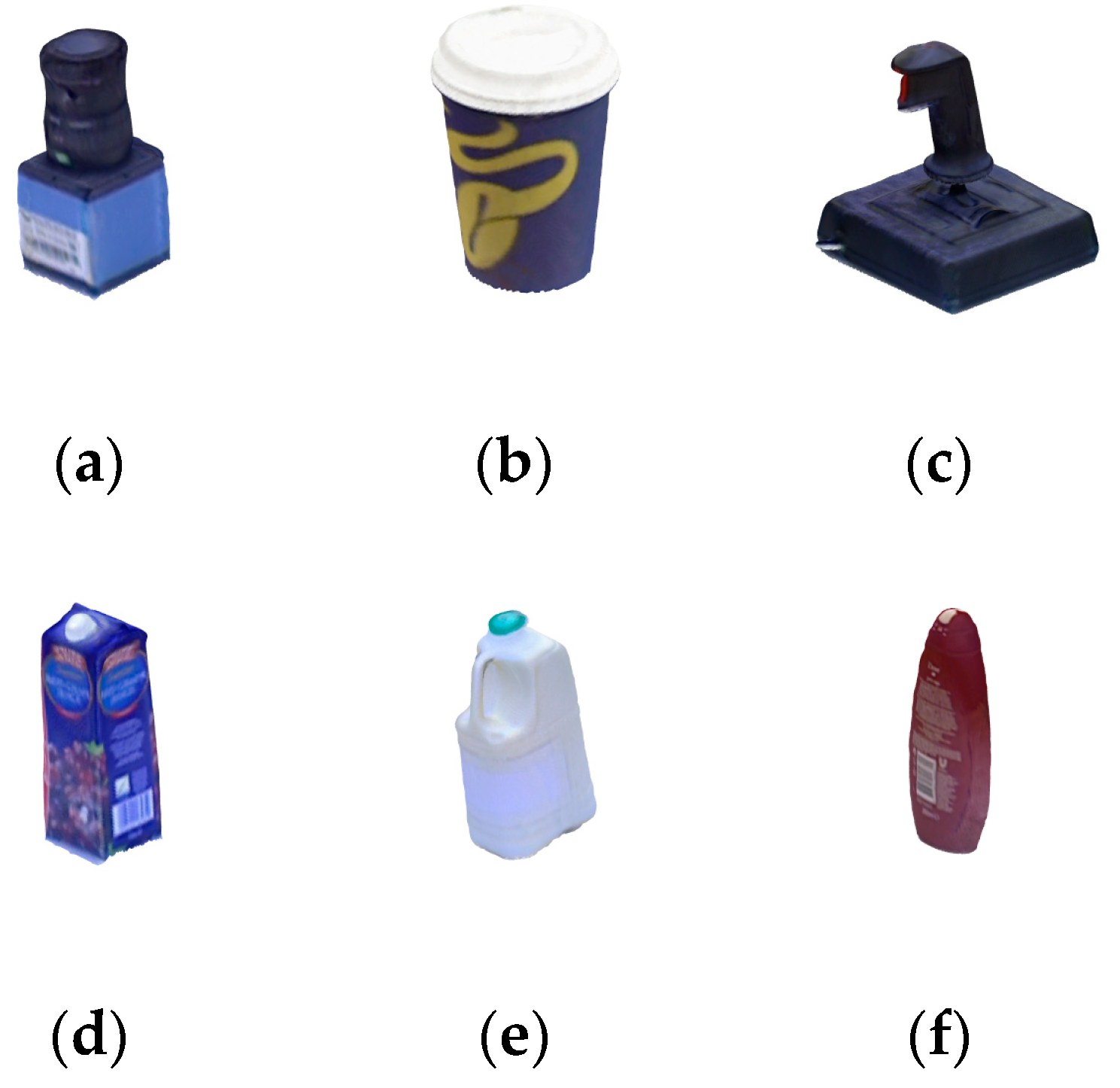
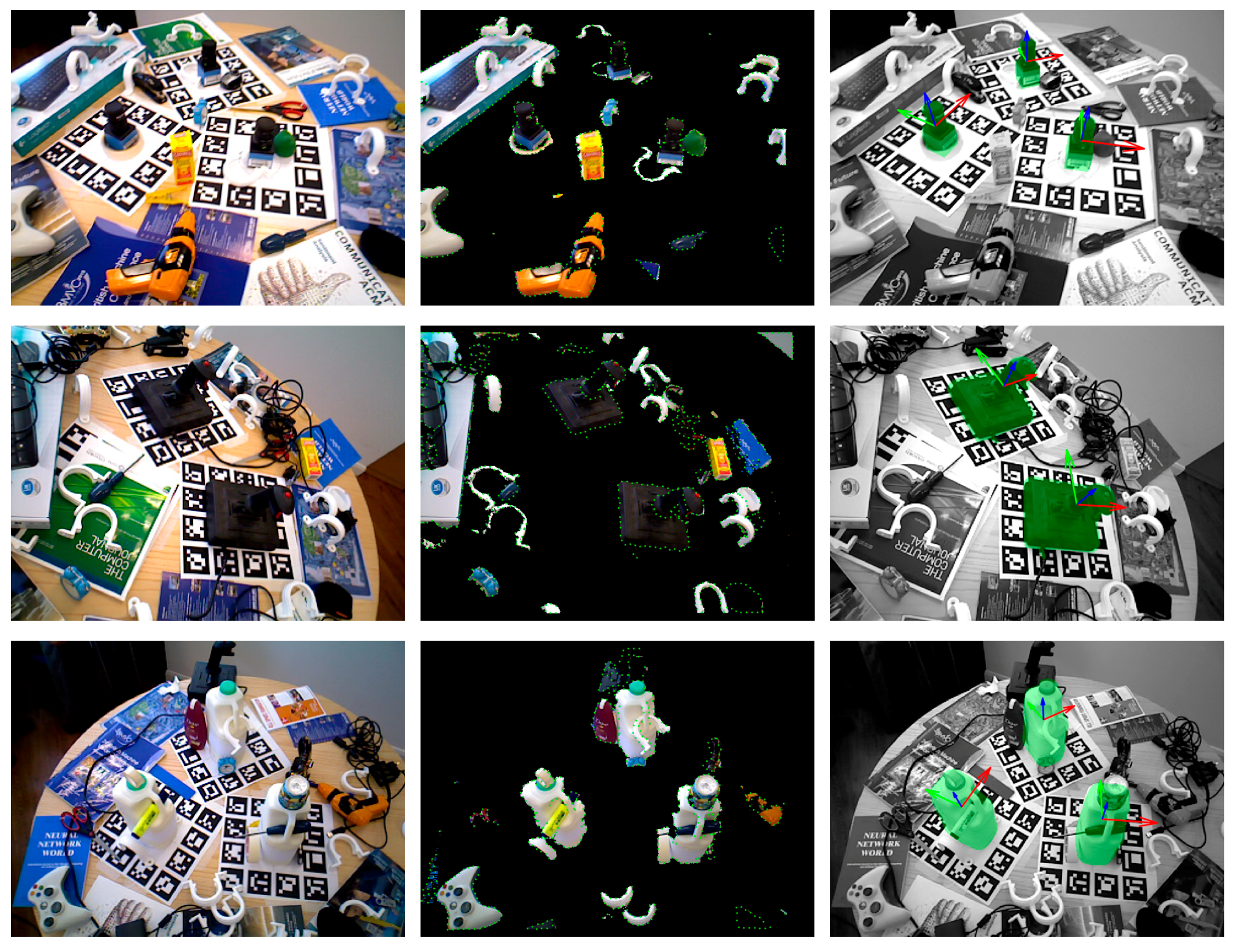
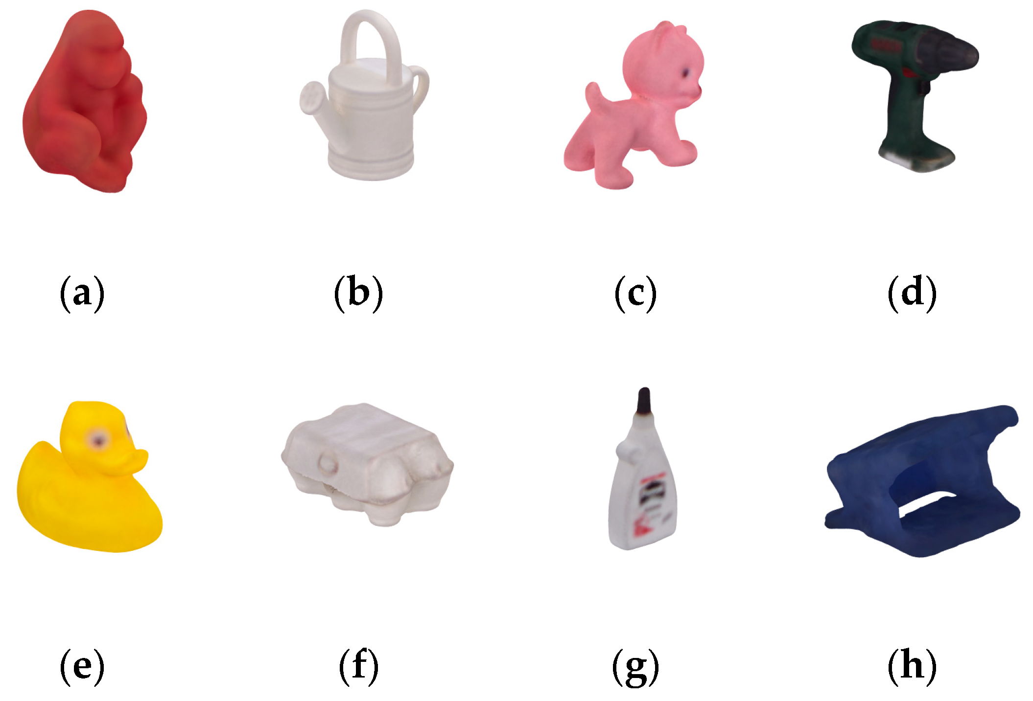
3.1. Results on the Tejani Dataset
3.1.1. Detection Results
3.1.2. Computation Time
3.2. Results on the Occlusion Dataset
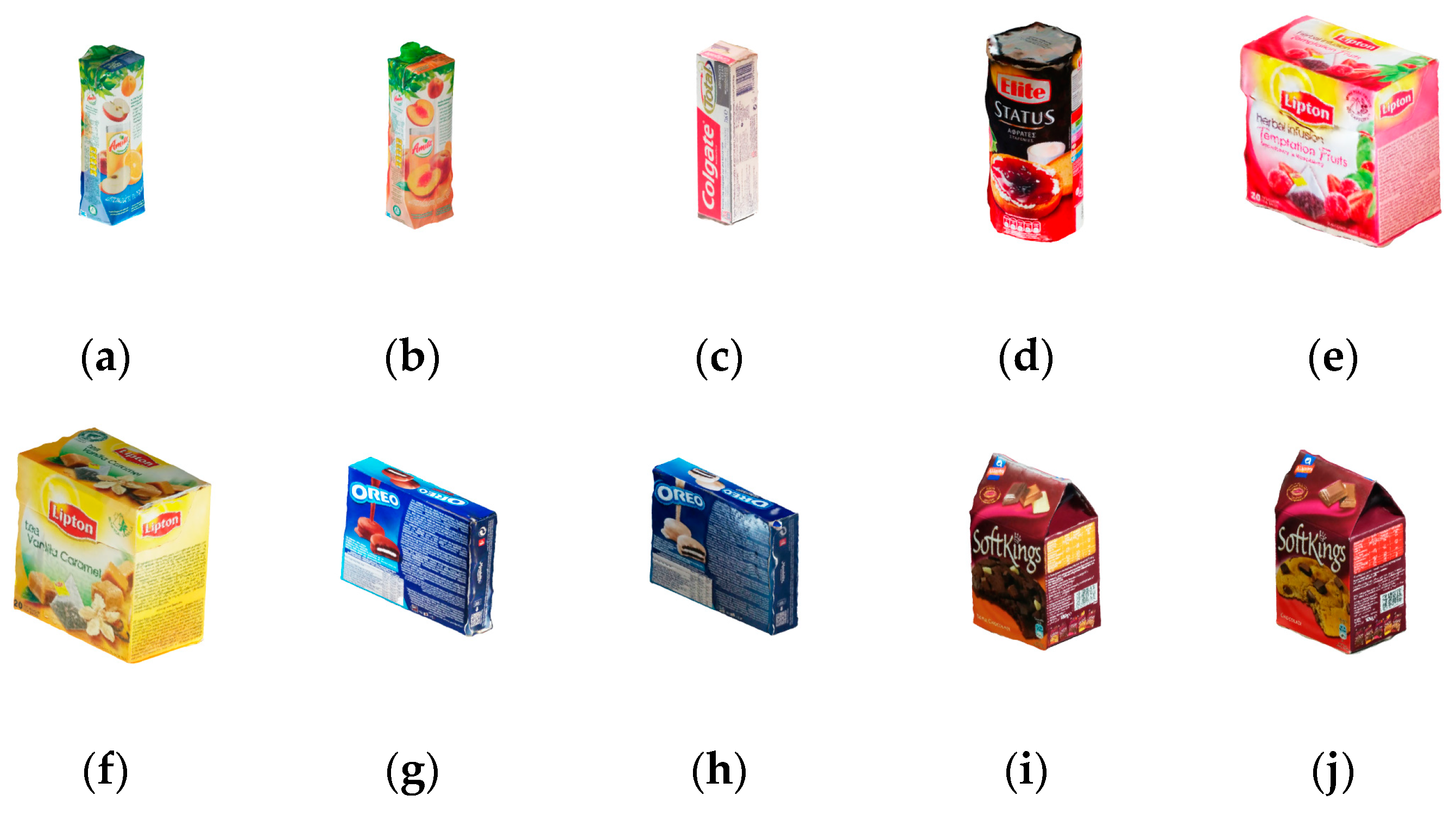
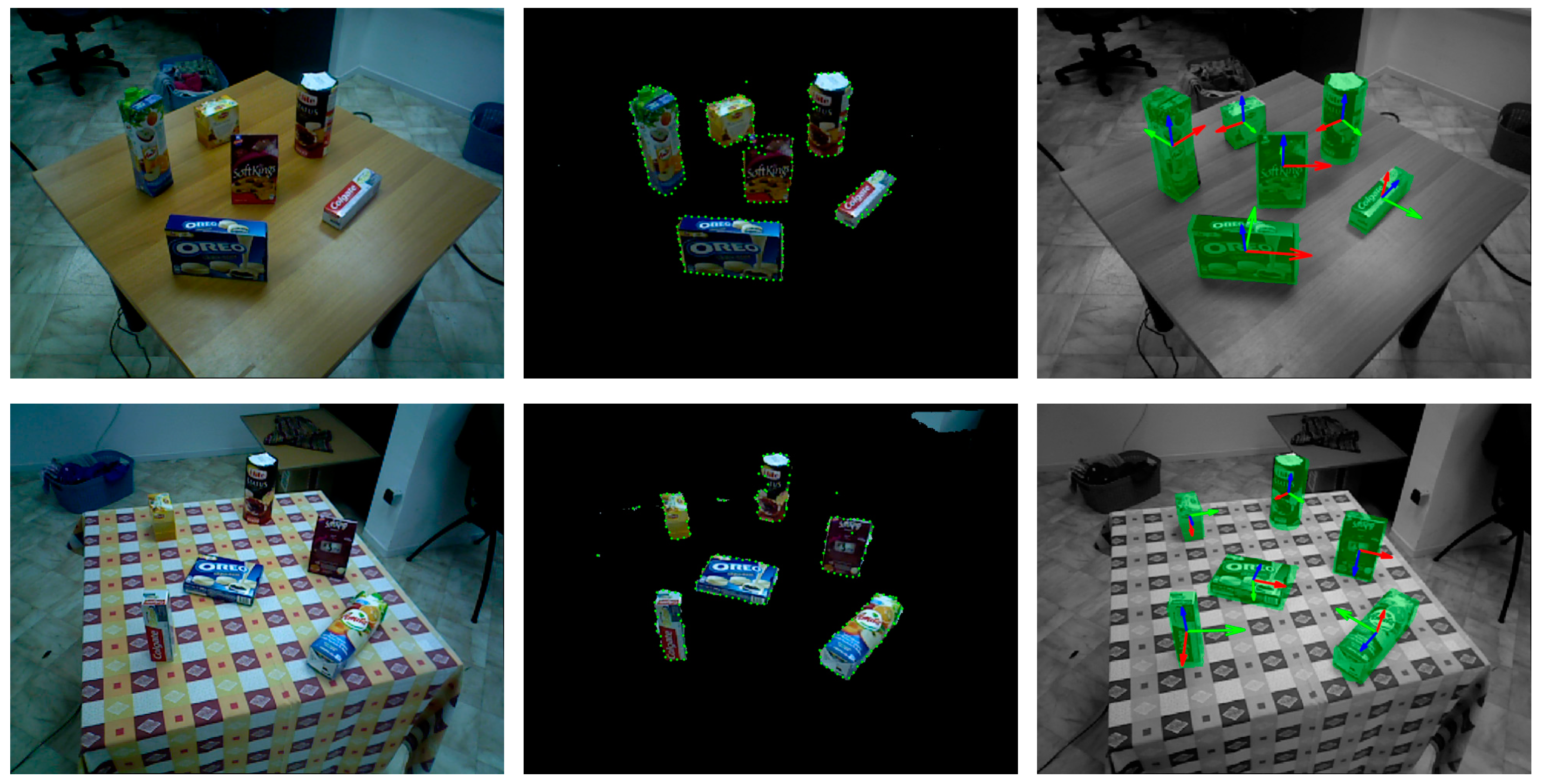
3.3. Results on the Doumanoglou Dataset
4. Conclusions
Author Contributions
Funding
Conflicts of Interest
References
- Tjaden, H.; Schwanecke, U.; Schomer, E. Real–time monocular pose estimation of 3D objects using temporally consistent local color histograms. In Proceedings of the IEEE International Conference on Computer Vision (ICCV), Venice, Italy, 22–29 October 2017. [Google Scholar]
- Hinterstoisser, S.; Cagniart, C.; Ilic, S.; Sturm, P.; Navab, N.; Fua, P.; Lepetit, V. Gradient response maps for real–time detection of textureless objects. IEEE. Trans. Pattern. Anal. 2011, 34, 876–888. [Google Scholar] [CrossRef] [PubMed]
- Hinterstoisser, S.; Holzer, S.; Cagniart, C.; Ilic, S.; Konolige, K.; Navab, N.; Lepetit, V. Multimodal templates for real–time detection of texture–less objects in heavily cluttered scenes. In Proceedings of the IEEE International Conference on Computer Vision (ICCV), Barcelona, Spain, 6–13 November 2011. [Google Scholar]
- Hinterstoisser, S.; Lepetit, V.; Ilic, S.; Holzer, S.; Bradski, G.; Konolige, K.; Navab, N. Model based training, detection and pose estimation of texture–less 3d objects in heavily cluttered scenes. In Proceedings of the 11th Asian Conference on Computer Vision (ACCV), Daejeon, Korea, 5–9 November 2012. [Google Scholar]
- Hodaň, T.; Zabulis, X.; Lourakis, M.; Obdržálek, Š.; Matas, J. Detection and fine 3D pose estimation of texture–less objects in RGB–D images. In Proceedings of the IEEE/RSJ International Conference on Intelligent Robots and Systems, Hamburg, Germany, 28 September–2 October 2015. [Google Scholar]
- Collet, A.; Martinez, M.; Srinivasa, S.S. The MOPED framework: Object recognition and pose estimation for manipulation. Int. J. Robot. Res. 2011, 30, 1284–1306. [Google Scholar] [CrossRef]
- Li, M.; Hashimoto, K. Accurate object pose estimation using depth only. Sensors 2018, 18, 1045–1061. [Google Scholar] [CrossRef] [PubMed]
- Vidal, J.; Lin, C.-Y.; Martí, R. 6D pose estimation using an improved method based on point pair features. In Proceedings of the 4th International Conference on Control, Automation and Robotics (ICCAR), Auckland, New Zealand, 20–23 April 2018. [Google Scholar]
- Drost, B.; Ulrich, M.; Navab, N.; Ilic, S. Model globally, match locally: Efficient and robust 3D object recognition. In Proceedings of the IEEE Computer Society Conference on Computer Vision and Pattern Recognition, San Francisco, CA, USA, 13–18 June 2010. [Google Scholar]
- Guo, Y.; Liu, Y.; Oerlemans, A.; Lao, S.; Wu, S.; Lew, M.S. Deep learning for visual understanding: A review. Neurocomputing 2016, 187, 27–48. [Google Scholar] [CrossRef]
- Bengio, Y.; Courville, A.C.; Vincent, P. Unsupervised feature learning and deep learning: A review and new perspectives. CoRR 2012, 1, 1–30. [Google Scholar]
- Voulodimos, A.; Doulamis, N.; Doulamis, A.; Protopapadakis, E. Deep learning for computer vision: A brief review. Comput. Intell. Neurosci. 2018, 2018, 1–13. [Google Scholar] [CrossRef] [PubMed]
- Michel, F.; Kirillov, A.; Brachmann, E.; Krull, A.; Gumhold, S.; Savchynskyy, B.; Rother, C. Global hypothesis generation for 6D object pose estimation. In Proceedings of the IEEE Conference on Computer Vision and Pattern Recognition (CVPR), Honolulu, HI, USA, 21–26 July 2017. [Google Scholar]
- Brachmann, E.; Krull, A.; Michel, F.; Gumhold, S.; Shotton, J.; Rother, C. Learning 6d object pose estimation using 3d object coordinates. In Proceedings of the 13th European Conference on Computer Vision (ECCV), Zurich, Switzerland, 6–12 September 2014. [Google Scholar]
- Brachmann, E.; Michel, F.; Krull, A.; Ying Yang, M.; Gumhold, S. Uncertainty–driven 6d pose estimation of objects and scenes from a single rgb image. In Proceedings of the IEEE Conference on Computer Vision and Pattern Recognition (CVPR), Las Vegas, NV, USA, 27–30 June 2016. [Google Scholar]
- Kehl, W.; Manhardt, F.; Tombari, F.; Ilic, S.; Navab, N. SSD–6D: Making RGB–based 3D detection and 6D pose estimation great again. In Proceedings of the IEEE International Conference on Computer Vision (ICCV), Venice, Italy, 22–29 October 2017. [Google Scholar]
- Rad, M.; Lepetit, V. BB8: A scalable, accurate, robust to partial occlusion method for predicting the 3D poses of challenging objects without using depth. In Proceedings of the IEEE International Conference on Computer Vision (ICCV), Venice, Italy, 22–29 October 2017. [Google Scholar]
- Tekin, B.; Sinha, S.N.; Fua, P. Real–time seamless single shot 6d object pose prediction. In Proceedings of the 2018 IEEE Conference on Computer Vision and Pattern Recognition (CVPR), Salt Lake City, UT, USA, 18–23 June 2018. [Google Scholar]
- Doumanoglou, A.; Kouskouridas, R.; Malassiotis, S.; Kim, T.-K. Recovering 6D object pose and predicting next–best–view in the crowd. In Proceedings of the IEEE Conference on Computer Vision and Pattern Recognition (CVPR), Las Vegas, NV, USA, 27–30 June 2016. [Google Scholar]
- Tejani, A.; Tang, D.; Kouskouridas, R.; Kim, T.-K. Latent–class hough forests for 3D object detection and pose estimation. In Proceedings of the 13th European Conference on Computer Vision (ECCV), Zurich, Switzerland, 6–12 September 2014. [Google Scholar]
- Kehl, W.; Milletari, F.; Tombari, F.; Ilic, S.; Navab, N. Deep learning of local RGB–D patches for 3D object detection and 6D pose estimation. In Proceedings of the 14th European Conference on Computer Vision (ECCV), Amsterdam, The Netherlands, 11–14 October 2016. [Google Scholar]
- Zhang, H.; Cao, Q. Texture–less object detection and 6D pose estimation in RGB–D images. Robot. Auton. Syst. 2017, 95, 64–79. [Google Scholar] [CrossRef]
- Fischler, M.A.; Bolles, R.C. Random sample consensus: A paradigm for model fitting with applications to image analysis and automated cartography. Commun. ACM 1981, 24, 381–395. [Google Scholar] [CrossRef]
- Liu, H.; Cong, Y.; Yang, C.; Tang, Y. Efficient 3D object recognition via geometric information preservation. Pattern Recognit. 2019, 92, 135–145. [Google Scholar] [CrossRef]
- Hodan, T.; Michel, F.; Brachmann, E.; Kehl, W.; GlentBuch, A.; Kraft, D.; Drost, B.; Vidal, J.; Ihrke, S.; Zabulis, X. BOP: Benchmark for 6D object pose estimation. In Proceedings of the 15th European Conference on Computer Vision (ECCV), Munich, Germany, 8–14 September 2018. [Google Scholar]


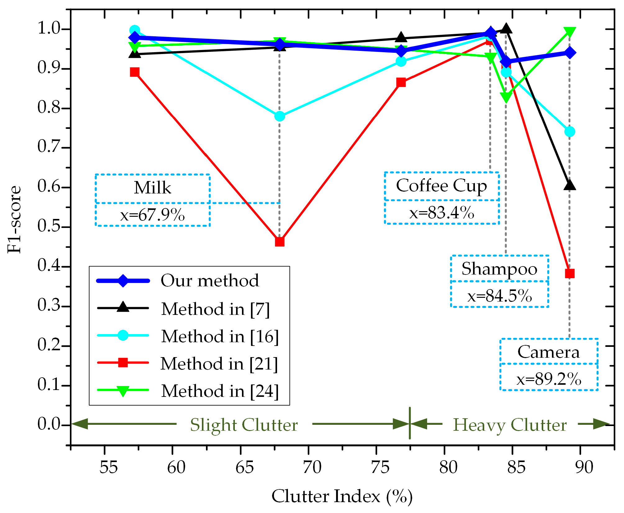
| Objects | Li et at. [7] | Kehl et al. [16] | Kehl et al. [21] | Liu et at. [24] | Ours |
|---|---|---|---|---|---|
| Camera | 0.603 | 0.741 | 0.383 | 0.996 | 0.941 |
| Coffee Cup | 0.991 | 0.983 | 0.972 | 0.931 | 0.990 |
| Joystick | 0.937 | 0.997 | 0.892 | 0.958 | 0.979 |
| Juice Carton | 0.977 | 0.919 | 0.866 | 0.949 | 0.945 |
| Milk | 0.954 | 0.780 | 0.463 | 0.970 | 0.962 |
| Shampoo | 0.999 | 0.892 | 0.910 | 0.831 | 0.918 |
| Average | 0.910 | 0.885 | 0.747 | 0.939 | 0.956 |
| Objects | Clutter Indexes |
|---|---|
| Joystick | 57.2 |
| Milk | 67.9 |
| Juice Carton | 76.8 |
| Coffee Cup | 83.4 |
| Shampoo | 84.5 |
| Camera | 89.2 |
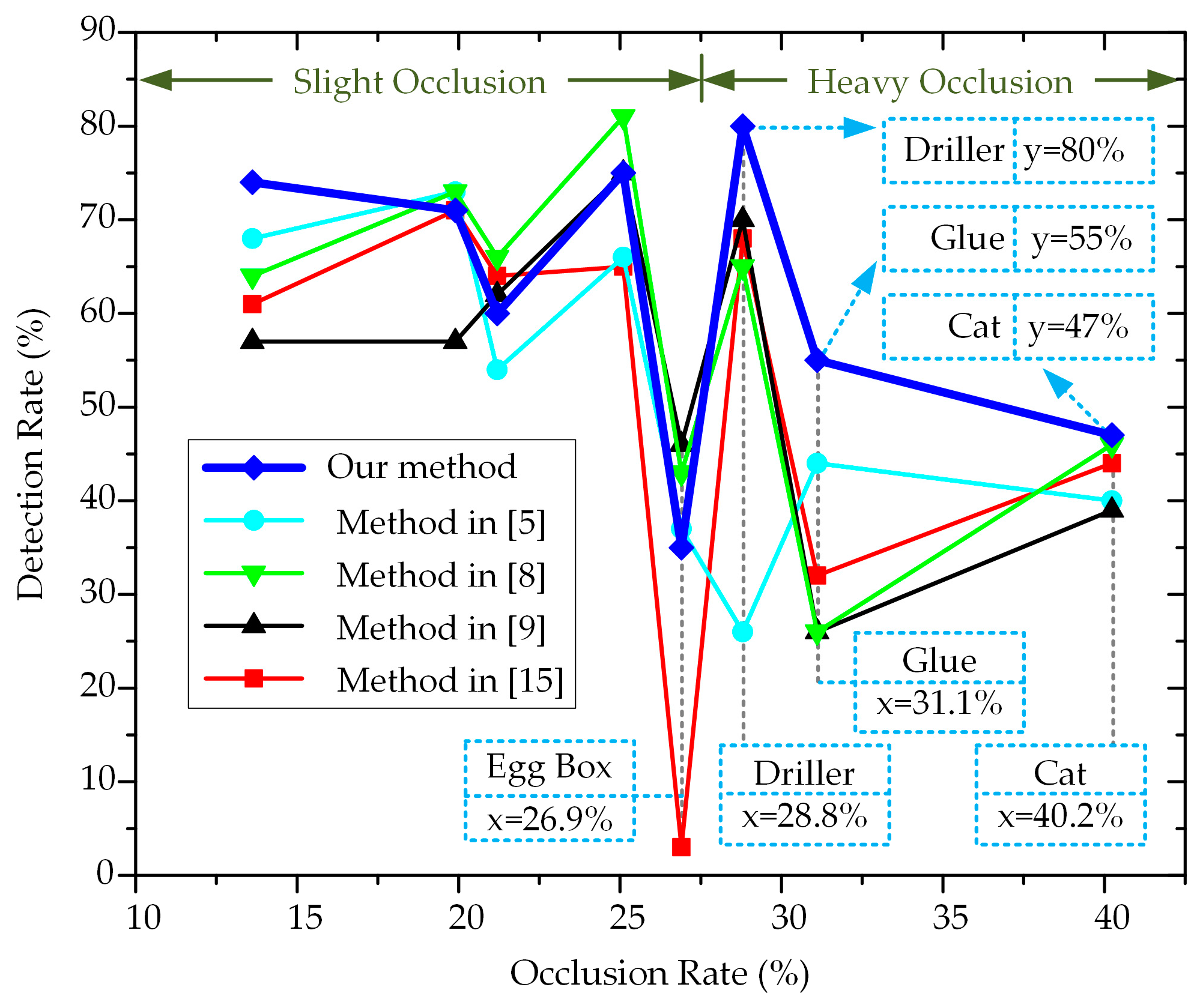
| Objects | Hodan et al. [5] | Vidal et al. [8] | Drost et al. [9] | Brachmann et al. [15] | Ours |
|---|---|---|---|---|---|
| Ape | 54 | 66 | 62 | 64 | 60 |
| Can | 66 | 81 | 75 | 65 | 75 |
| Cat | 40 | 46 | 39 | 44 | 47 |
| Driller | 26 | 65 | 70 | 68 | 80 |
| Duck | 73 | 73 | 57 | 71 | 71 |
| Egg Box | 37 | 43 | 46 | 3 | 35 |
| Glue | 44 | 26 | 26 | 32 | 55 |
| Hole Punch | 68 | 64 | 57 | 61 | 74 |
| Average | 51 | 58 | 54 | 51 | 62 |
| Objects | Occlusion Rates |
|---|---|
| Hole Punch | 13.6 |
| Duck | 19.9 |
| Ape | 21.2 |
| Can | 25.1 |
| Egg Box | 26.9 |
| Driller | 28.8 |
| Glue | 31.1 |
| Cat | 40.2 |
| Objects | Clutter Indexes |
|---|---|
| Amita | 13.6 |
| Colgate | 55.5 |
| Elite | 8.3 |
| Lipton | 56.1 |
| Oreo | 22.3 |
| Soft Kings | 25.5 |
| Objects | Doumanoglou et at. [19] | Ours |
|---|---|---|
| Amita | 71.2 | 72.5 |
| Colgate | 28.6 | 53.6 |
| Elite | 77.6 | 85.7 |
| Lipton | 59.2 | 78.6 |
| Oreo | 59.3 | 87.5 |
| Soft Kings | 75.9 | 91.1 |
| Average | 62.0 | 78.2 |
© 2020 by the authors. Licensee MDPI, Basel, Switzerland. This article is an open access article distributed under the terms and conditions of the Creative Commons Attribution (CC BY) license (http://creativecommons.org/licenses/by/4.0/).
Share and Cite
Tong, X.; Li, R.; Ge, L.; Zhao, L.; Wang, K. A New Edge Patch with Rotation Invariance for Object Detection and Pose Estimation. Sensors 2020, 20, 887. https://doi.org/10.3390/s20030887
Tong X, Li R, Ge L, Zhao L, Wang K. A New Edge Patch with Rotation Invariance for Object Detection and Pose Estimation. Sensors. 2020; 20(3):887. https://doi.org/10.3390/s20030887
Chicago/Turabian StyleTong, Xunwei, Ruifeng Li, Lianzheng Ge, Lijun Zhao, and Ke Wang. 2020. "A New Edge Patch with Rotation Invariance for Object Detection and Pose Estimation" Sensors 20, no. 3: 887. https://doi.org/10.3390/s20030887
APA StyleTong, X., Li, R., Ge, L., Zhao, L., & Wang, K. (2020). A New Edge Patch with Rotation Invariance for Object Detection and Pose Estimation. Sensors, 20(3), 887. https://doi.org/10.3390/s20030887