Simulation of SAW Sensors with Various Distributed Mass Loadings Using Two-Dimensional Coupling-of-Modes Theory


Abstract
:1. Introduction
2. Methods
2.1. Two-Dimensional Coupling-of-Modes Equations
2.2. Two-Dimensional Finite Element Model of the SAW Sensor Chip
2.3. Two-Dimensional COM Parameters
2.4. Generalized PDE Form of 2-D COM Equations
2.5. Admittance Matrix and Insertion Loss
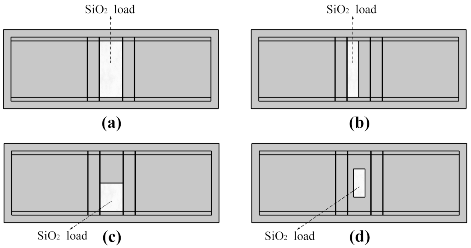
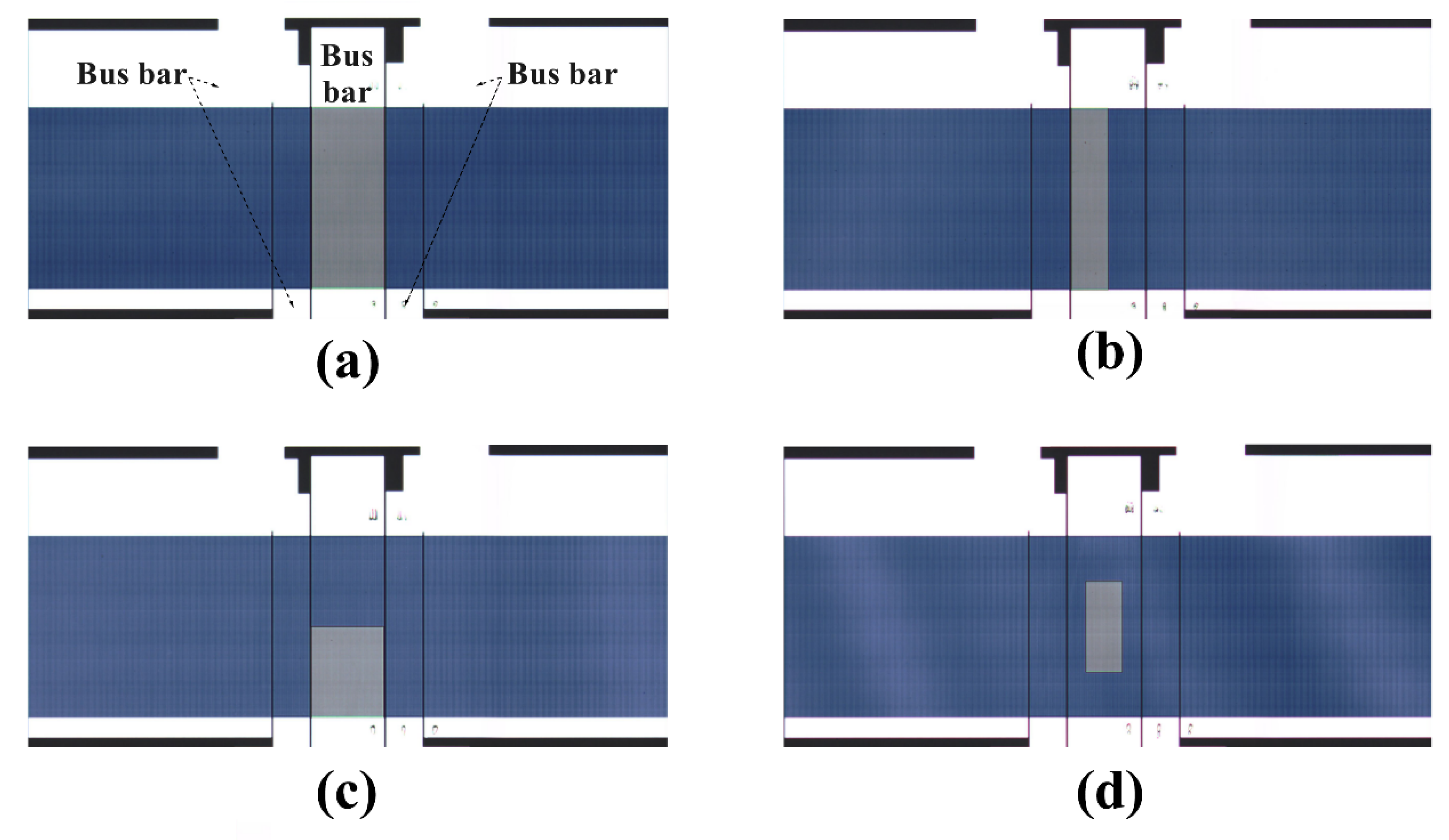
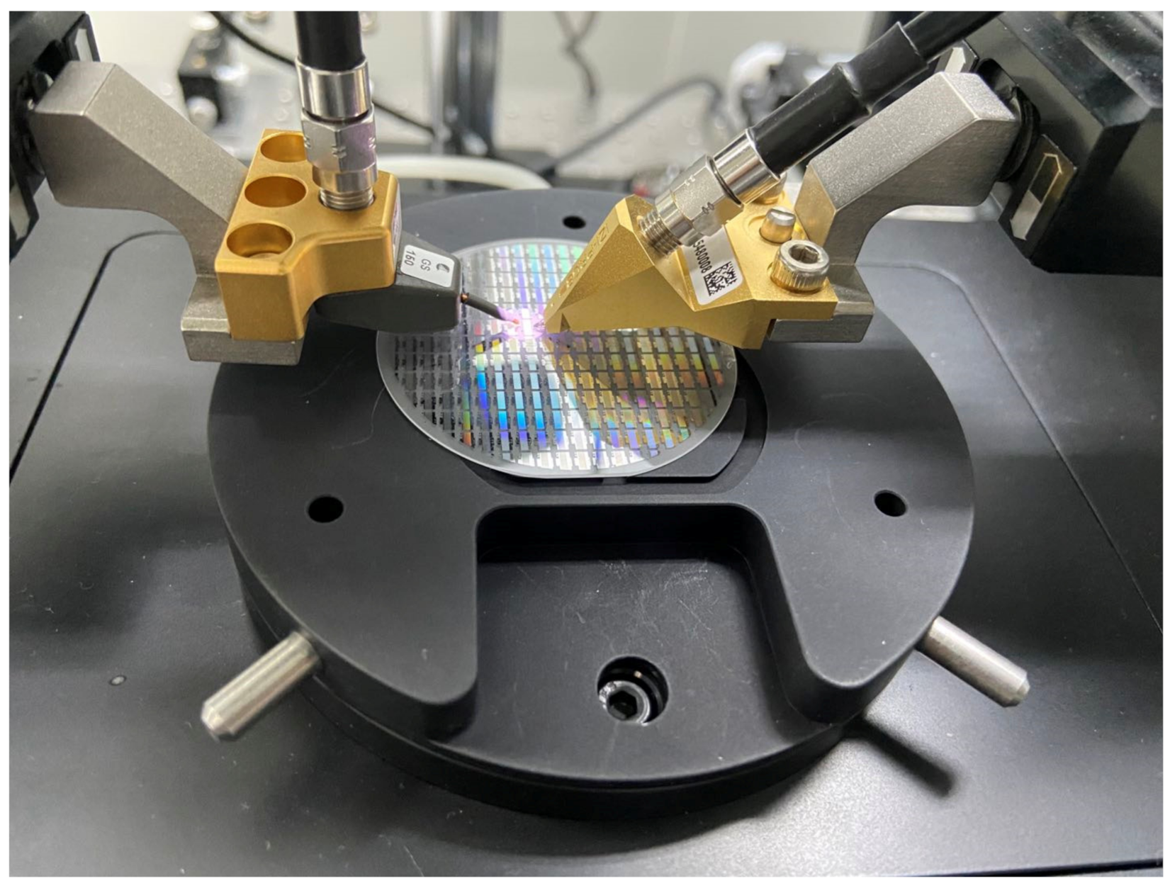
2.6. Experimental Design
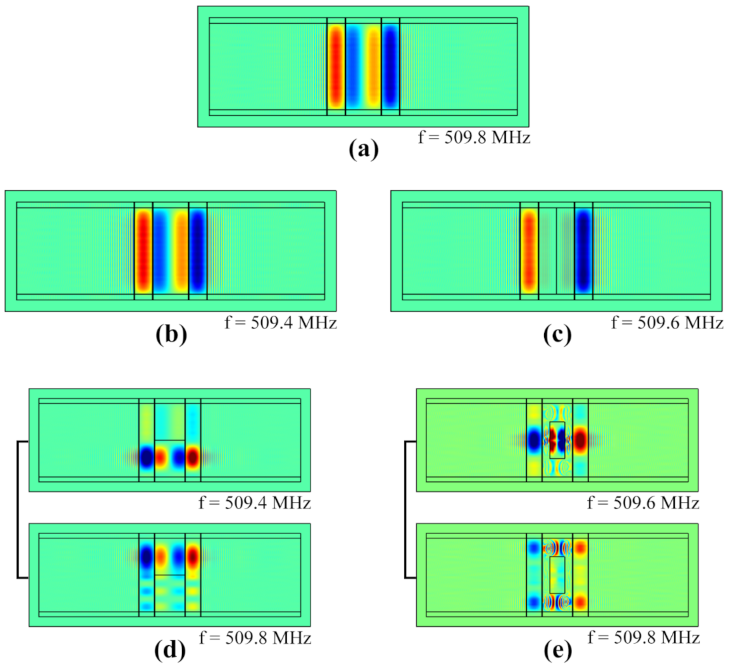
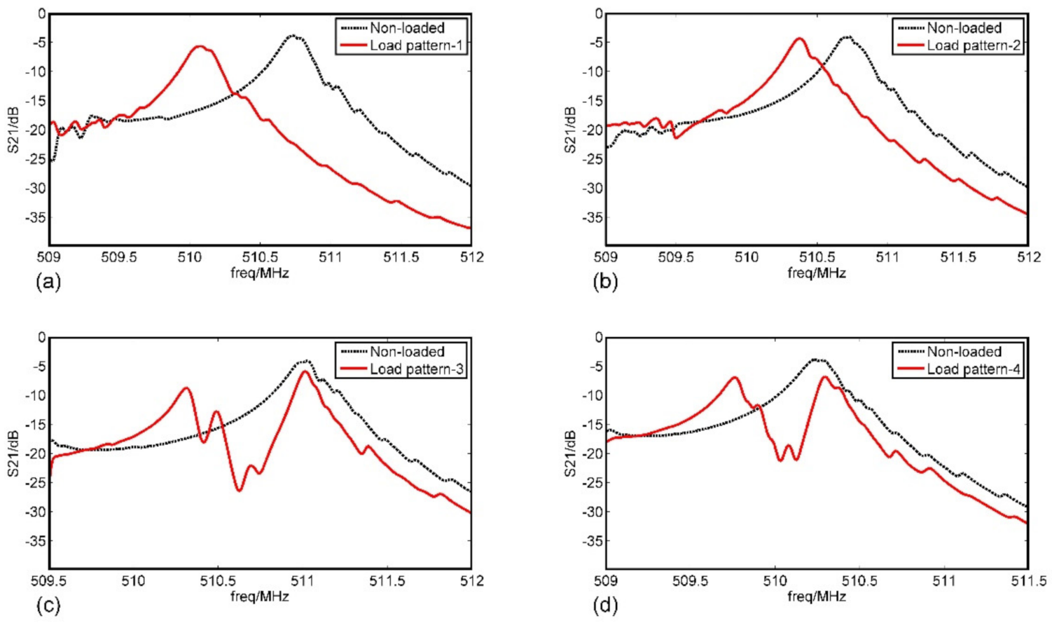
3. Results and Discussion
4. Conclusions
Author Contributions
Funding
Conflicts of Interest
References
- Plessky, V.; Koskela, J. Coupling-of-modes analysis of saw devices. Int. J. High Speed Electron. Syst. 2000, 10, 867–947. [Google Scholar] [CrossRef]
- Haus, H.A. Modes in SAW grating resonators. J. Appl. Phys. 1977, 48, 4955–4961. [Google Scholar] [CrossRef]
- Haus, H.A.; Wang, K.L. Modes of grating waveguide. J. Appl. Phys. 1978, 49, 1061–1069. [Google Scholar] [CrossRef]
- Bergmann, A.; Wagner, K.; Mayer, M.; Riha, G. 6D-5 A 2D P-Matrix Model for the Simulation of Waveguiding and Diffraction in SAW Components (Invited). In Proceedings of the 2006 IEEE Ultrasonics Symposium, Vancouver, BC, Canada, 2–6 October 2006; IEEE: Vancouver, BC, Canada, 2006; pp. 380–388. [Google Scholar]
- Hirota, O.T.K. Two-Dimensional Coupling-of-Modes Analysis in Surface Acoustic Wave Device Performed by COMSOL Multiphysics. Jpn. J. Appl. Phys. 2011, 4. [Google Scholar] [CrossRef]
- Xiao, Q.; Ji, X.; Ma, X.; Cai, P. A New General Form of 2-D Coupling-of-Modes Equations for Analysis of Waveguiding in Surface Acoustic Wave Devices. IEEE Trans. Ultrason. Ferroelect. Freq. Contr. 2020, 67, 1033–1039. [Google Scholar] [CrossRef] [PubMed]
- Länge, K.; Rapp, B.E.; Rapp, M. Surface acoustic wave biosensors: A review. Anal. Bioanal. Chem. 2008, 391, 1509–1519. [Google Scholar] [CrossRef] [PubMed]
- Gronewold, T.M.A. Surface acoustic wave sensors in the bioanalytical field: Recent trends and challenges. Anal. Chim. Acta 2007, 603, 119–128. [Google Scholar] [CrossRef] [PubMed]
- Saitakis, M.; Gizeli, E. Acoustic sensors as a biophysical tool for probing cell attachment and cell/surface interactions. Cell. Mol. Life Sci. 2012, 69, 357–371. [Google Scholar] [CrossRef] [PubMed]
- Liu, J.; Wang, W.; Li, S.; Liu, M.; He, S. Advances in SAW Gas Sensors Based on the Condensate-Adsorption Effect. Sensors 2011, 11, 11871–11884. [Google Scholar] [CrossRef] [PubMed]
- Ding, X.; Li, P.; Lin, S.C.S.; Stratton, Z.S.; Nama, N.; Guo, F.; Slotcavage, D.; Mao, X.; Shi, J.; Costanzo, F.; et al. Surface acoustic wave microfluidics. Lab Chip 2013, 13, 3626. [Google Scholar] [CrossRef] [PubMed]
- Drbohlavová, L.; Fekete, L.; Bovtun, V.; Kempa, M.; Taylor, A.; Liu, Y.; Bou Matar, O.; Talbi, A.; Mortet, V. Love-wave devices with continuous and discrete nanocrystalline diamond coating for biosensing applications. Sens. Actuators A Phys. 2019, 298, 111584. [Google Scholar] [CrossRef]
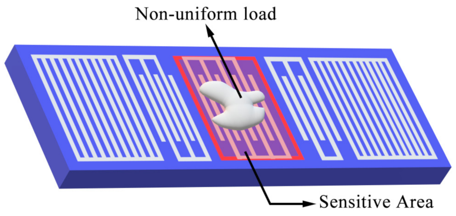
- You, R.; Liu, J.; Liu, M.; He, S. Detecting of non-uniformly distributed loads with SAW sensors using a two-dimensional segmentation method. 2020; Under Review. [Google Scholar]
- Hirota, K.; Nakamura, K. Analysis of SAW Grating Waveguides using 2-D Coupling-of-Modes equations. In Proceedings of the 2001 IEEE Ultrasonics Symposium Proceedings. An International Symposium (Cat. No.01CH37263), Atlanta, GA, USA, 7–10 October 2001; pp. 115–120. [Google Scholar] [CrossRef]


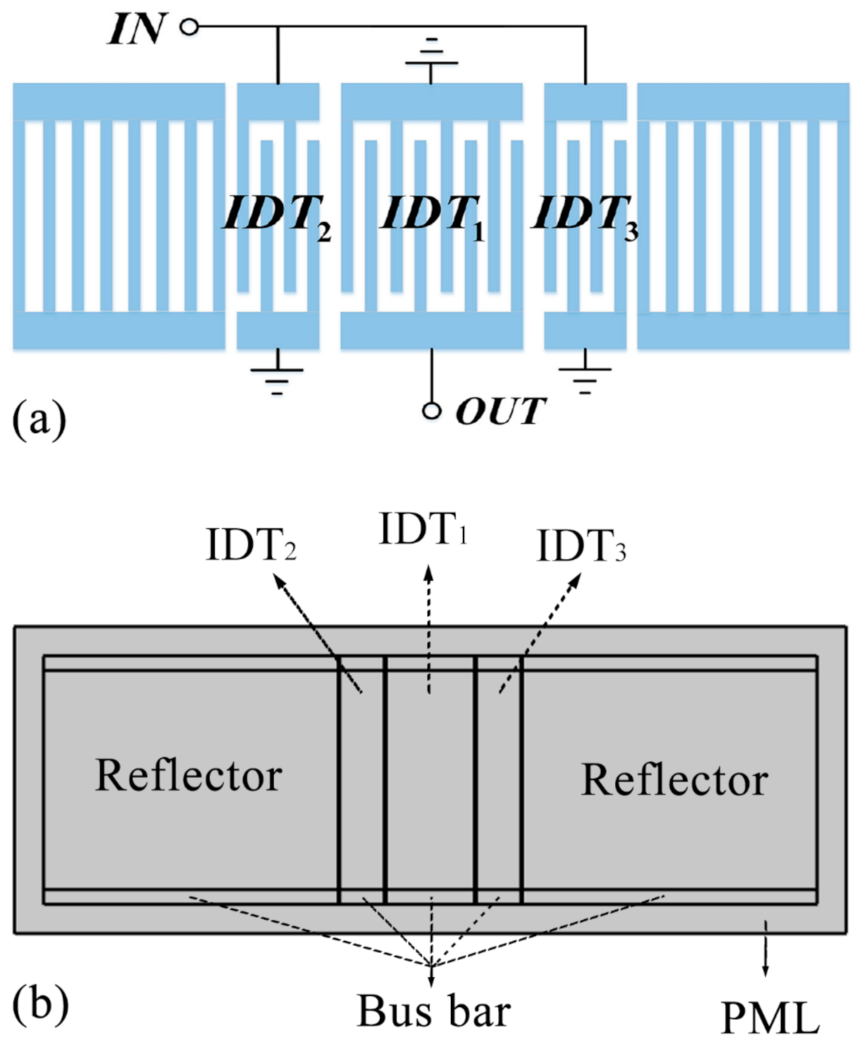
| Structural Parameters | Value |
|---|---|
| Period (λ) | 6.074 (μm) |
| Aperture | 150*λ |
| Width of busbar | 10*λ |
| Length of Gaps between IDTs | 1.25*λ |
| Length of Gaps between IDT and reflector | 1*λ |
| Number of fingers in IDT1 | 121 |
| Number of fingers in IDT2,3 | 61 |
| Number of fingers in reflector | 401 |
| Substrate Material: ST-X Quartz | |
|---|---|
| Period (λ) | 6.074 (μm) |
| Thickness of IDTs | 2000 (Å) |
| Metallization ratio | 0.5 |
| Thickness of loads | 1000 (Å) |
| 1-D COM Parameters | Non-Loaded | Loaded |
|---|---|---|
| SAW velocity | 3126 (m/s) | 3124 (m/s) |
| Normalized reflection coefficient | 0.040 | 0.044 |
| Normalized excitation coefficient | 2.49 × 10⁻⁵ | 2.31 × 10⁻⁵ |
| Static capacitance | 4.00 × 10⁻¹¹ (F) | 4.48 × 10⁻¹¹ (F) |
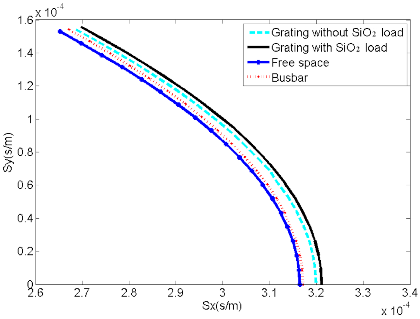
| Domains | ||
|---|---|---|
| Grating | −1.3754 | −0.3988 |
| Grating with SiO2 load | −1.3499 | −0.6601 |
| Busbar | −1.3366 | −0.1233 |
| Free space | −1.3928 | 0.1871 |
| Elements of Y Matrix | Short-Circuited IDTs |
|---|---|
| Y11 | IDT1 |
| Y12 | IDT2, IDT3 |
| Y21 | IDT1 |
| Y22 | IDT2, IDT3 |
| Parameters | Value |
|---|---|
| Substrate material | ST-X Quartz |
| Load material | SiO2 |
| Grating material | Al |
| Thickness of gratings | 2000 (Å) |
| Thickness of loads | 1000 (Å) |
Publisher’s Note: MDPI stays neutral with regard to jurisdictional claims in published maps and institutional affiliations. |
© 2020 by the authors. Licensee MDPI, Basel, Switzerland. This article is an open access article distributed under the terms and conditions of the Creative Commons Attribution (CC BY) license (http://creativecommons.org/licenses/by/4.0/).
Share and Cite
You, R.; Liu, J.; Liu, M.; Chen, Z.; He, S. Simulation of SAW Sensors with Various Distributed Mass Loadings Using Two-Dimensional Coupling-of-Modes Theory. Sensors 2020, 20, 7260. https://doi.org/10.3390/s20247260
You R, Liu J, Liu M, Chen Z, He S. Simulation of SAW Sensors with Various Distributed Mass Loadings Using Two-Dimensional Coupling-of-Modes Theory. Sensors. 2020; 20(24):7260. https://doi.org/10.3390/s20247260
Chicago/Turabian StyleYou, Ran, Jiuling Liu, Minghua Liu, Zhiyuan Chen, and Shitang He. 2020. "Simulation of SAW Sensors with Various Distributed Mass Loadings Using Two-Dimensional Coupling-of-Modes Theory" Sensors 20, no. 24: 7260. https://doi.org/10.3390/s20247260
APA StyleYou, R., Liu, J., Liu, M., Chen, Z., & He, S. (2020). Simulation of SAW Sensors with Various Distributed Mass Loadings Using Two-Dimensional Coupling-of-Modes Theory. Sensors, 20(24), 7260. https://doi.org/10.3390/s20247260