Author Contributions
Conceptualization, D.I.G., R.C.A. and C.T.; methodology, D.I.G., A.W.H. and C.T.; software, D.I.G., A.W.H., X.B. and C.T.; validation, D.I.G., A.W.H., X.B. and C.T.; formal analysis, D.I.G.; investigation, D.I.G.; resources, D.I.G., X.B. and C.M.; data curation, D.I.G.; writing—original draft preparation, D.I.G.; writing—review and editing, D.I.G., C.T., C.M. and I.A.; visualization, D.I.G.; supervision, C.T. and I.A.; project administration, D.I.G., C.M. and R.C.A.; funding acquisition, D.I.G. and C.T. All authors have read and agreed to the published version of the manuscript.
Figure 1.
Delaminations (a) locations shown in red for the sample panel D8, (b) PTFE inclusion between the two laminate plies during lay up of sample panel D8.
Figure 1.
Delaminations (a) locations shown in red for the sample panel D8, (b) PTFE inclusion between the two laminate plies during lay up of sample panel D8.
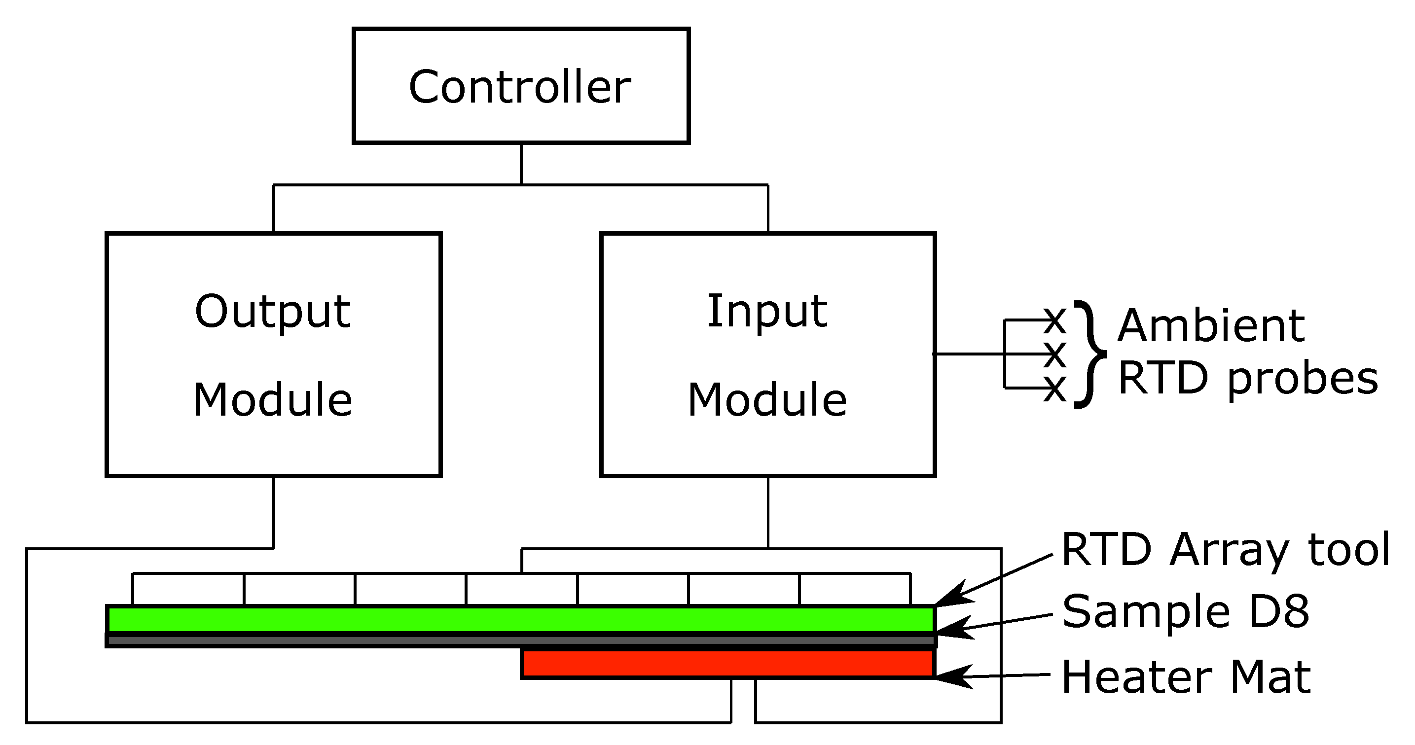
Figure 2.
Experimental set up showing the Controller, Input module, Output module, Ambient RTD Probes, RTD array, sample D8 and heater mat.
Figure 2.
Experimental set up showing the Controller, Input module, Output module, Ambient RTD Probes, RTD array, sample D8 and heater mat.
Figure 3.
Heater mat locations for D8, displayed in dashed lines and RTD array position 1 with corresponding RTD sensors numbered with location shown in a blue ’x’ (a) Heater mat positions 6–10 (b) Heater mat positions 1–5.
Figure 3.
Heater mat locations for D8, displayed in dashed lines and RTD array position 1 with corresponding RTD sensors numbered with location shown in a blue ’x’ (a) Heater mat positions 6–10 (b) Heater mat positions 1–5.
Figure 4.
Heater mat locations for D8, displayed as dashed lines and RTD array position 2 with corresponding RTD probes numbered and locations shown in a blue ‘x’ (a) Heater mat positions 6–10 (b) Heater mat positions 1–5.
Figure 4.
Heater mat locations for D8, displayed as dashed lines and RTD array position 2 with corresponding RTD probes numbered and locations shown in a blue ‘x’ (a) Heater mat positions 6–10 (b) Heater mat positions 1–5.
Figure 5.
Thermal profile for heater mat and step heating profile.
Figure 5.
Thermal profile for heater mat and step heating profile.
Figure 6.
Thermal profile for probes in D8 at y_heat_dist of ≤37.5 mm and x_heat_dist of 0 mm.
Figure 6.
Thermal profile for probes in D8 at y_heat_dist of ≤37.5 mm and x_heat_dist of 0 mm.
Figure 7.
Thermal profile for probes in D8 at y_heat_dist of ≤37.5 mm and x_heat_dist of 18.75 mm.
Figure 7.
Thermal profile for probes in D8 at y_heat_dist of ≤37.5 mm and x_heat_dist of 18.75 mm.
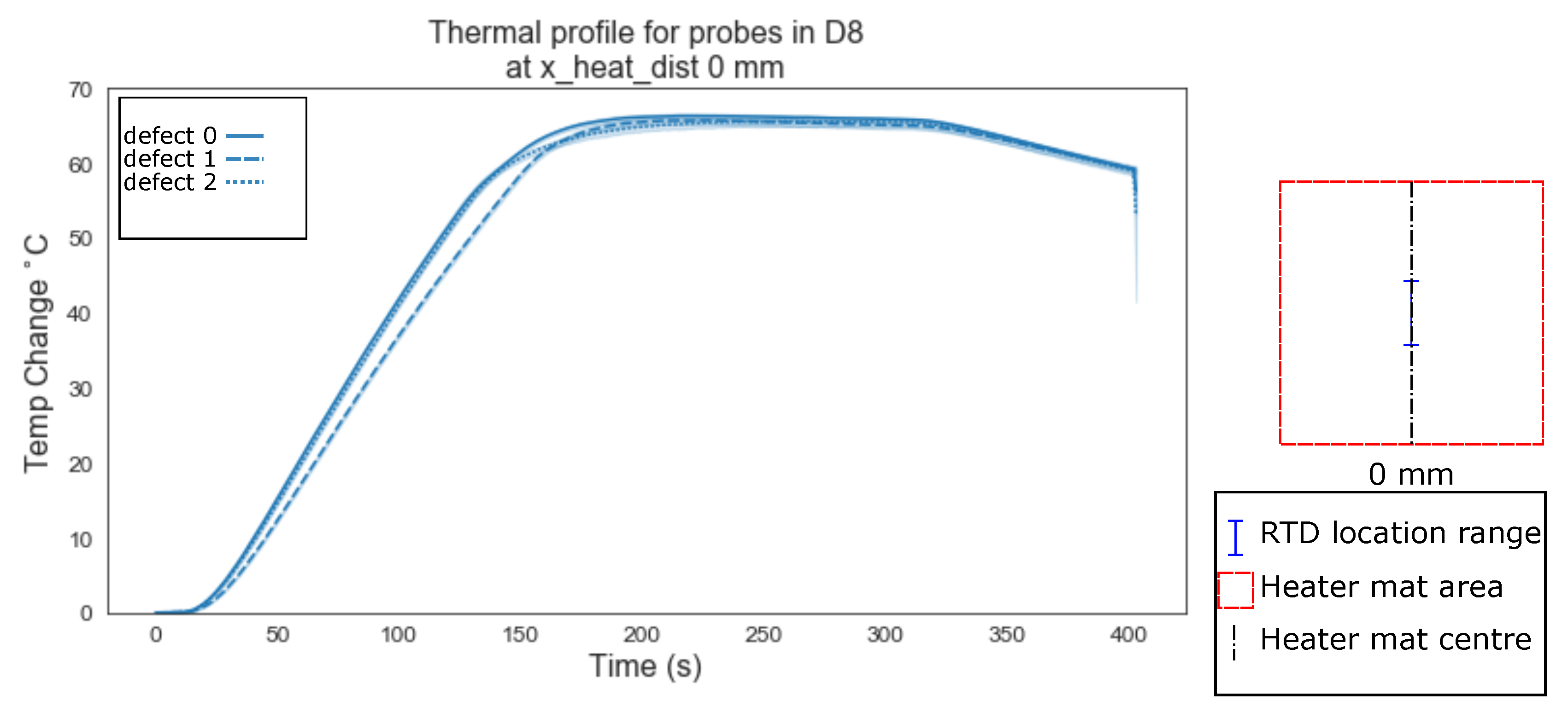
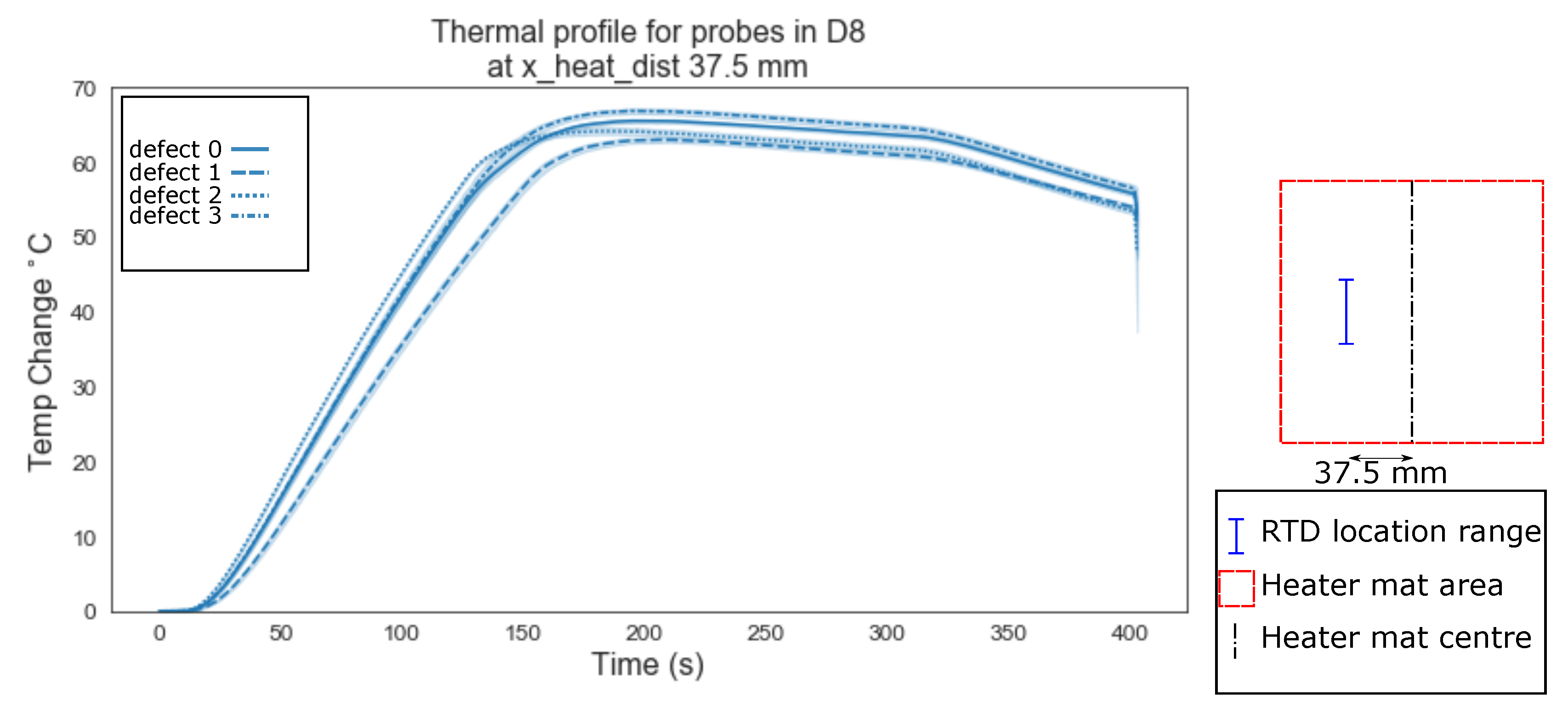
Figure 8.
Thermal profile for probes in D8 at y_heat_dist of ≤37.5 mm and x_heat_dist of 37.5 mm.
Figure 8.
Thermal profile for probes in D8 at y_heat_dist of ≤37.5 mm and x_heat_dist of 37.5 mm.
Figure 9.
Thermal profile for probes in D8 at y_heat_dist of ≤37.5 mm and x_heat_dist of 56.25 mm.
Figure 9.
Thermal profile for probes in D8 at y_heat_dist of ≤37.5 mm and x_heat_dist of 56.25 mm.
Figure 10.
Thermal profile for probes in D8 at y_heat_dist of ≤37.5 mm and x_heat_dist of 75 mm.
Figure 10.
Thermal profile for probes in D8 at y_heat_dist of ≤37.5 mm and x_heat_dist of 75 mm.
Figure 11.
Thermal profile for probes in D8 at y_heat_dist of ≤37.5 mm and x_heat_dist of 93.75 mm.
Figure 11.
Thermal profile for probes in D8 at y_heat_dist of ≤37.5 mm and x_heat_dist of 93.75 mm.
Figure 12.
Thermal profiles for probes in D8 at y_heat_dist of ≤37.5 mm and x_heat_dist of 112.5 mm.
Figure 12.
Thermal profiles for probes in D8 at y_heat_dist of ≤37.5 mm and x_heat_dist of 112.5 mm.
Figure 13.
Confusion matrix of validation data set for SVC algorithm with RBF kernel, C = 0.1 and = 0.1, using all data points.
Figure 13.
Confusion matrix of validation data set for SVC algorithm with RBF kernel, C = 0.1 and = 0.1, using all data points.
Figure 14.
Confusion matrix of validation data set, for SVC algorithm with RBF kernel, C = 0.1 and = 0.1, using all data points from the balanced data set.
Figure 14.
Confusion matrix of validation data set, for SVC algorithm with RBF kernel, C = 0.1 and = 0.1, using all data points from the balanced data set.
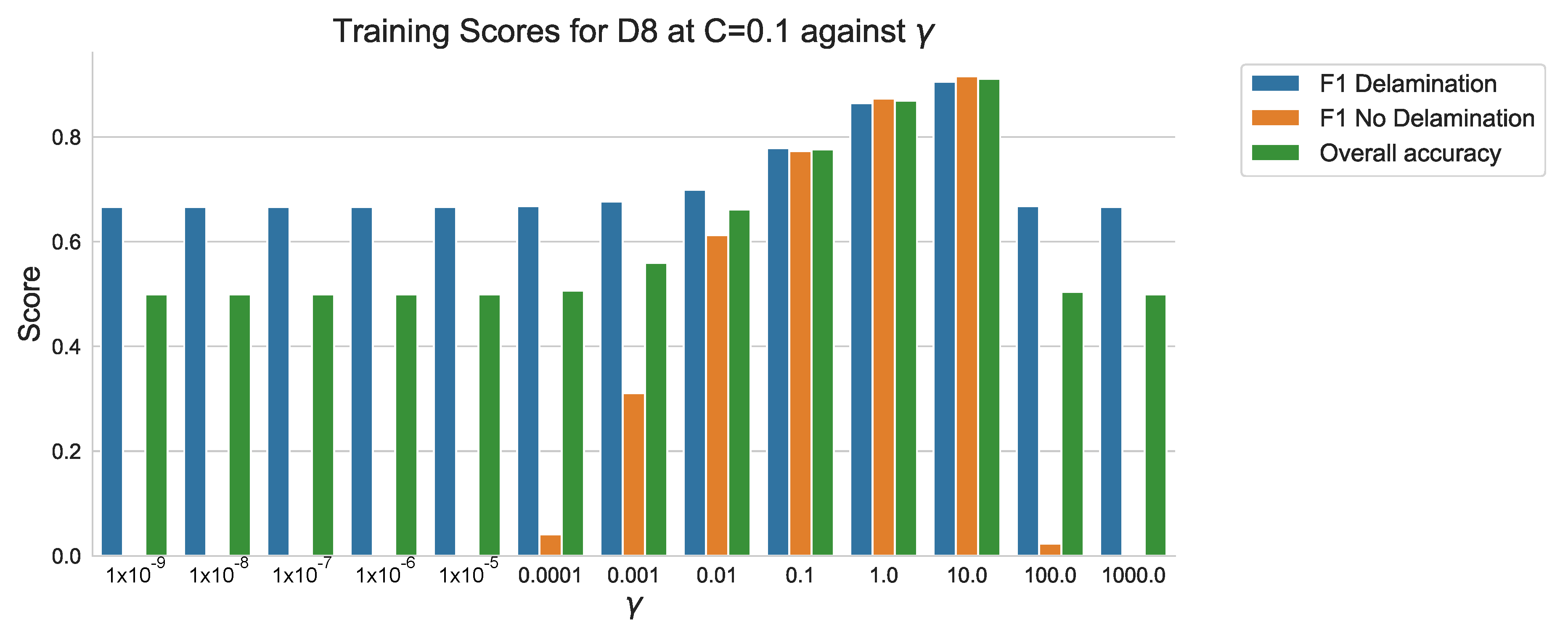
Figure 15.
F1 scores and overall accuracy of sample D8 within training data set using SVM algorithms with RBF kernel, C = 0.1 values against .
Figure 15.
F1 scores and overall accuracy of sample D8 within training data set using SVM algorithms with RBF kernel, C = 0.1 values against .
Figure 16.
Confusion matrix for SVC algorithm with RBF kernel, C = 0.1 and = 10.0, using all data points from the balanced data set.
Figure 16.
Confusion matrix for SVC algorithm with RBF kernel, C = 0.1 and = 10.0, using all data points from the balanced data set.
Figure 17.
Training classification scores against ‘x_dist’.
Figure 17.
Training classification scores against ‘x_dist’.
Figure 18.
Testing classification scores against ‘x_dist’.
Figure 18.
Testing classification scores against ‘x_dist’.
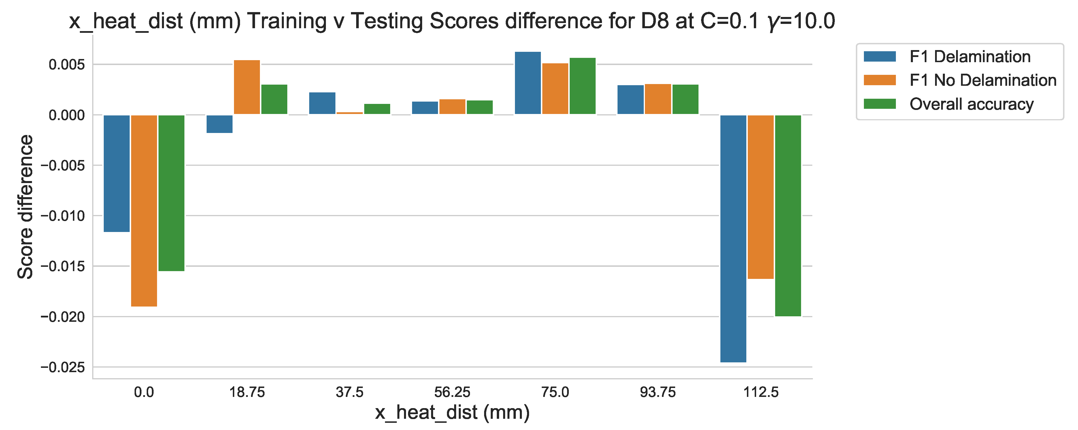
Figure 19.
Training v Testing classification scores difference against ‘x_dist’.
Figure 19.
Training v Testing classification scores difference against ‘x_dist’.
Figure 20.
Display of overall percentage score (0–1) of the 140 time intervals for each RTD probes which classified as ‘No Delamination’ (a) Corresponding RTD probe locations, (b) Gaussian filter application to present image similar to traditional IR thermography methods.
Figure 20.
Display of overall percentage score (0–1) of the 140 time intervals for each RTD probes which classified as ‘No Delamination’ (a) Corresponding RTD probe locations, (b) Gaussian filter application to present image similar to traditional IR thermography methods.
Table 1.
Pandas Dataframe of dataset showing the first five rows and column headers.
Table 1.
Pandas Dataframe of dataset showing the first five rows and column headers.
| | Temp | Time (s) | x_heat_dist | y_heat_dist | std_140 | Mean | Median | heat_mat_temp | amb_1 | amb_2 | amb_3 | Defect |
|---|
| | Change C | | | | | | | | | | | |
|---|
| 0 | 0.1 | 20 | 75.0 | 0.0 | 6.068788 | 0.218182 | 0.1 | 29.8 | 24.5 | 24.3 | 24.2 | 0.0 |
| 1 | 0.1 | 21 | 75.0 | 0.0 | 6.068788 | 0.265455 | 0.1 | 30.5 | 24.5 | 24.3 | 24.2 | 0.0 |
| 2 | 0.2 | 22 | 75.0 | 0.0 | 6.068788 | 0.309091 | 0.1 | 31.0 | 24.5 | 24.3 | 24.2 | 0.0 |
| 3 | 0.2 | 23 | 75.0 | 0.0 | 6.068788 | 0.369091 | 0.1 | 31.5 | 24.5 | 24.3 | 24.2 | 0.0 |
| 4 | 0.2 | 24 | 75.0 | 0.0 | 6.068788 | 0.438182 | 0.1 | 32.1 | 24.5 | 24.3 | 24.2 | 0.0 |
Table 2.
Pandas Dataframe of data set showing the first five rows and column headers of Training data set.
Table 2.
Pandas Dataframe of data set showing the first five rows and column headers of Training data set.
| | Temp Change C | Time (s) | x_heat_dist | y_heat_dist | std_140 | Mean | Median | heat_mat_temp | amb_1 | amb_2 | amb_3 |
|---|
| 0 | 0.1 | 20 | 75.0 | 0.0 | 6.068788 | 0.218182 | 0.1 | 29.8 | 24.5 | 24.3 | 24.2 |
| 1 | 0.1 | 21 | 75.0 | 0.0 | 6.068788 | 0.265455 | 0.1 | 30.5 | 24.5 | 24.3 | 24.2 |
| 2 | 0.2 | 22 | 75.0 | 0.0 | 6.068788 | 0.309091 | 0.1 | 31.0 | 24.5 | 24.3 | 24.2 |
| 3 | 0.2 | 23 | 75.0 | 0.0 | 6.068788 | 0.369091 | 0.1 | 31.5 | 24.5 | 24.3 | 24.2 |
| 4 | 0.2 | 24 | 75.0 | 0.0 | 6.068788 | 0.438182 | 0.1 | 32.1 | 24.5 | 24.3 | 24.2 |
Table 3.
Classification Report of validation data set for SVC algorithm with RBF kernel, C = 0.1 and = 0.1, using all data points.
Table 3.
Classification Report of validation data set for SVC algorithm with RBF kernel, C = 0.1 and = 0.1, using all data points.
| | F1-Score | Precision | Recall | Support |
|---|
| Delamination | 0.000000 | 0.000000 | 0.00000 | 21,441.00000 |
| No Delamination | 0.884725 | 0.793280 | 1.00000 | 82,279.00000 |
| accuracy | 0.793280 | | | |
| macro avg | 0.442363 | 0.396640 | 0.50000 | 103,720.00000 |
| weighted avg | 0.701835 | 0.629293 | 0.79328 | 103,720.00000 |
Table 4.
Classification Report of validation data set, for SVC algorithm with RBF kernel, C = 0.1 and = 0.1, using all data points from the balanced data set.
Table 4.
Classification Report of validation data set, for SVC algorithm with RBF kernel, C = 0.1 and = 0.1, using all data points from the balanced data set.
| | F1-Score | Precision | Recall | Support |
|---|
| Delamination | 0.778363 | 0.768689 | 0.788284 | 21,458.000000 |
| No Delamination | 0.773293 | 0.783378 | 0.763465 | 21,519.000000 |
| accuracy | 0.775857 | | | |
| macro avg | 0.775828 | 0.776033 | 0.775874 | 42,977.000000 |
| weighted avg | 0.775825 | 0.776044 | 0.775857 | 42,977.000000 |
Table 5.
Classification Report for SVC algorithm with RBF kernel, C = 0.1 and = 10.0, using all data points from the balanced data set.
Table 5.
Classification Report for SVC algorithm with RBF kernel, C = 0.1 and = 10.0, using all data points from the balanced data set.
| | F1-Score | Precision | Recall | Support |
|---|
| Delamination | 0.905525 | 0.961901 | 0.855392 | 21,458.000000 |
| No Delamination | 0.915665 | 0.870140 | 0.966216 | 21,519.000000 |
| accuracy | 0.910883 | | | |
| macro avg | 0.910595 | 0.916021 | 0.910804 | 42,977.000000 |
| weighted avg | 0.910602 | 0.915956 | 0.910883 | 42,977.000000 |
Table 6.
Classification Report for ‘x_heat_dist’ at 56.25 mm validation data set, for SVC algorithm with RBF kernel, C = 0.1 and = 10.0, trained on balanced data set.
Table 6.
Classification Report for ‘x_heat_dist’ at 56.25 mm validation data set, for SVC algorithm with RBF kernel, C = 0.1 and = 10.0, trained on balanced data set.
| | F1-Score | Precision | Recall | Support |
|---|
| Delamination | 0.992484 | 0.993978 | 0.990994 | 2665.000000 |
| No Delamination | 0.992427 | 0.990926 | 0.993932 | 2637.000000 |
| accuracy | 0.992456 | | | |
| macro avg | 0.992456 | 0.992452 | 0.992463 | 5302.000000 |
| weighted avg | 0.992456 | 0.992460 | 0.992456 | 5302.000000 |

 ,
, 


