Frequency Domain Panoramic Imaging Algorithm for Ground-Based ArcSAR

 ,
,
Abstract
1. Introduction
2. Geometry, Signal Model, and Resolution
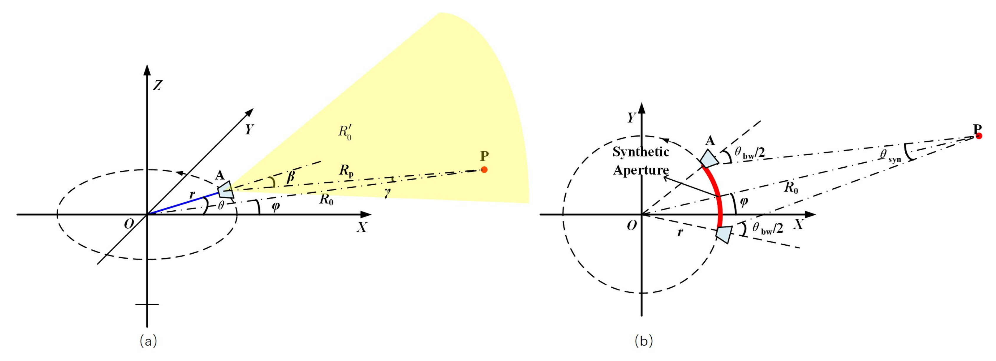
2.1. Geometry of ArcSAR
2.2. Signal Model of ArcSAR
2.3. Resolution of ArcSAR
3. Frequency Domain Panoramic Imaging Algorithm
3.1. 2-D Frequency Domain Signal
3.2. 2-D Matched Filter in the 2-D Frequency Domain
3.3. Range Variant Correction Function in the Range and Angular Frequency Domain
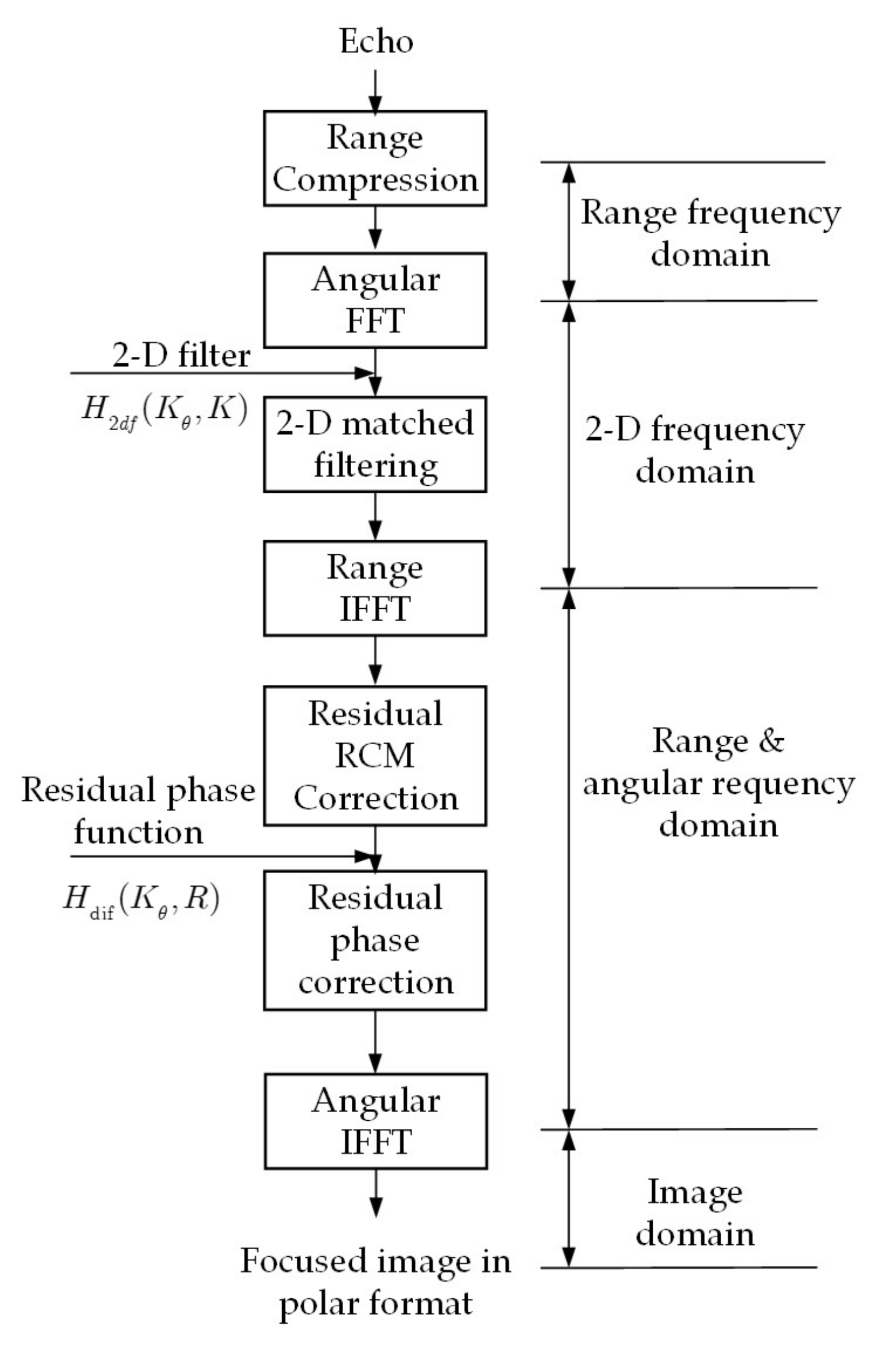
3.4. Algorithm Flow
3.5. Errors Caused by the Proposed Algorithm
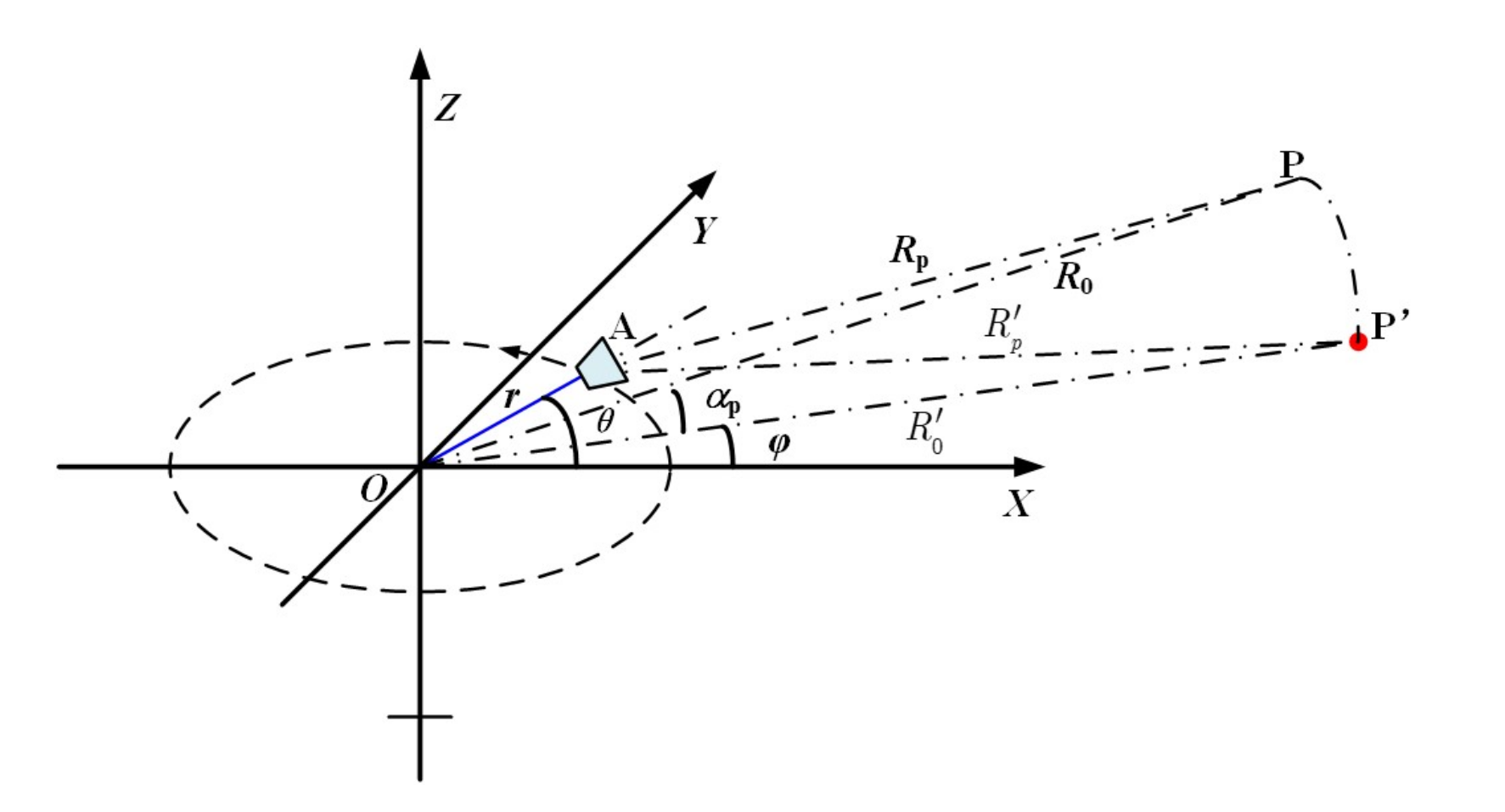
3.6. Errors Caused by Reference Plane Imaging
4. Experiments
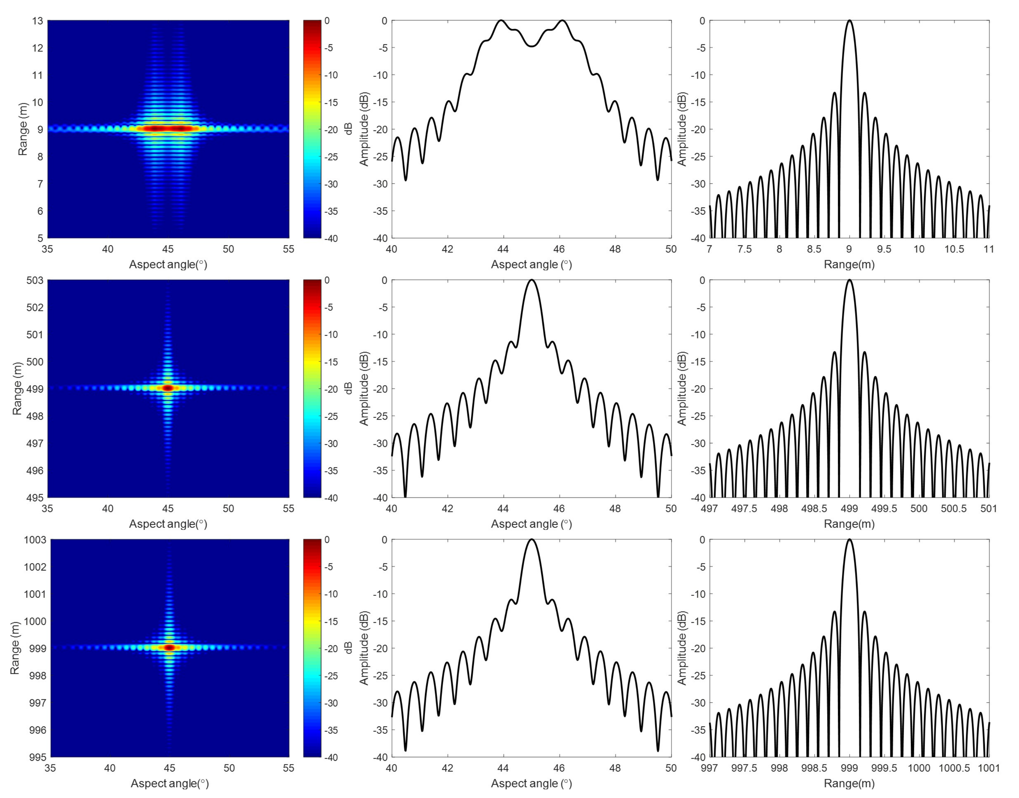
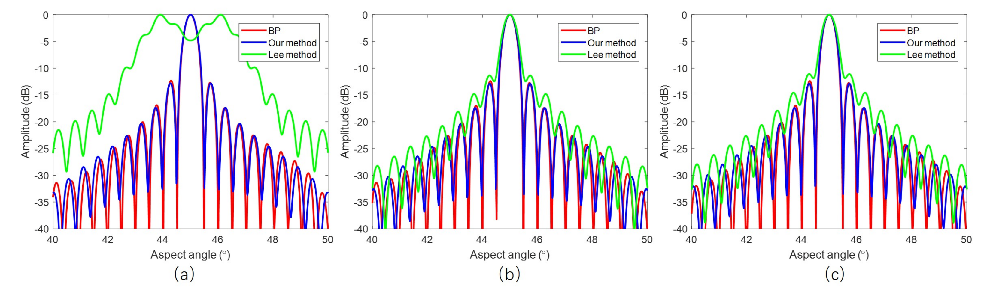
4.1. Simulation
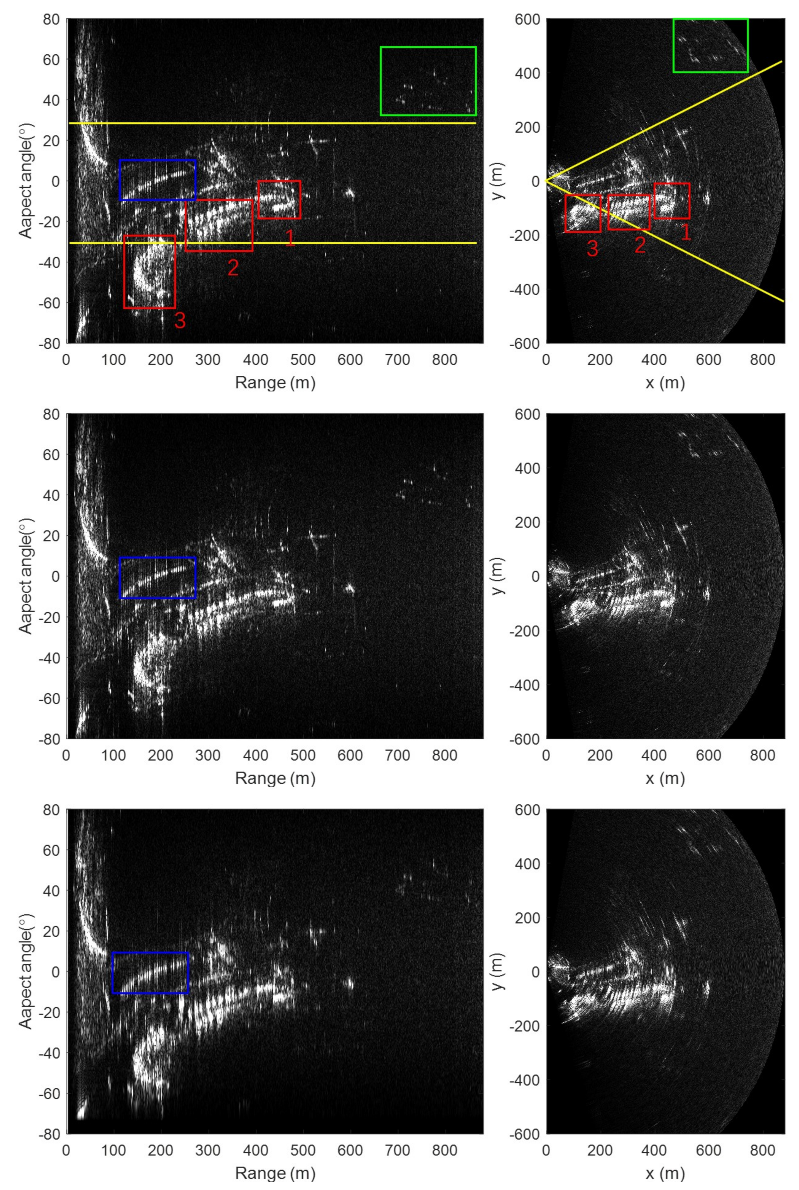
4.2. Real Data
5. Conclusions
Author Contributions
Funding
Conflicts of Interest
References
- Tarchi, D.; Casagli, N.; Fanti, R.; Leva, D.D.; Luzi, G.; Pasuto, A.; Pieraccini, M.; Silvano, S. Landslide monitoring by using ground-based SAR interferometry: An example of application to the Tessina landslide in Italy. Eng. Geol. 2003, 68, 15–30. [Google Scholar] [CrossRef]
- Pieraccini, M.; Miccinesi, L. Ground-based radar interferometry: A bibliographic review. Remote Sens. 2019, 11, 1029. [Google Scholar] [CrossRef]
- Wang, Y.P.; Hong, W.; Zhang, Y.; Lin, Y.; Li, Y.; Bai, Z.C.; Zhang, Q.M.; L, S.V.; Liu, H.; Song, Y. Ground-Based Differential Interferometry SAR: A Review. IEEE Geosci. Remote Sens. Mag. 2020, 8, 43–70. [Google Scholar] [CrossRef]
- Iglesias, R.; Aguasca, A.; Fabregas, X.; Mallorqui, J.J.; Monells, D.; Lopez-Martinez, C.; Pipia, L. Ground-Based Polarimetric SAR Interferometry for the Monitoring of Terrain Displacement Phenomena-Part I: Theoretical Description. IEEE J. Sel. Top. Appl. Earth Obs. Remote Sens. 2015, 8, 980–993. [Google Scholar] [CrossRef]
- Iglesias, R.; Aguasca, A.; Fabregas, X.; Mallorqui, J.J.; Monells, D.; Lopez-Martinez, C.; Pipia, L. Ground-Based Polarimetric SAR Interferometry for the Monitoring of Terrain Displacement Phenomena-Part II: Applications. IEEE J. Sel. Top. Appl. Earth Obs. Remote Sens. 2015, 8, 994–1007. [Google Scholar] [CrossRef]
- De Santis, R.; Gloria, A.; Viglione, S.; Maietta, S.; Nappi, F.; Ambrosio, L.; Ronca, D. 3D laser scanning in conjunction with surface texturing to evaluate shift and reduction of the tibiofemoral contact area after meniscectomy. J. Mech. Behav. Biomed. Mater. 2018, 88, 41–47. [Google Scholar] [CrossRef] [PubMed]
- Gao, R.P.; Zhou, B.; Ye, F.; Wang, Y.Z. Fast and Resilient Indoor Floor Plan Construction with a Single User. IEEE Trans. Mob. Comput. 2019, 18, 1083–1097. [Google Scholar] [CrossRef]
- Pieraccini, M.; Miccinesi, L. ArcSAR: Theory, Simulations, and Experimental Verification. IEEE Trans. Microw. Theory Tech. 2017, 65, 293–301. [Google Scholar] [CrossRef]
- Wang, Y.P.; Song, Y.; Lin, Y.; Li, Y.; Zhang, Y.; Hong, W. Interferometric DEM-Assisted High Precision Imaging Method for ArcSAR. Sensors 2019, 19, 2921. [Google Scholar] [CrossRef] [PubMed]
- Viviani, F.; Michelini, A.; Mayer, L.; Coppi, F. IBIS-ArcSAR: An Innovative Ground-Based SAR System for Slope Monitoring. In Proceedings of the Igarss 2018-2018 IEEE International Geoscience and Remote Sensing Symposium, Valencia, Spain, 22–27 July 2018; pp. 1348–1351. [Google Scholar]
- Fortuny-Guasch, J. A Fast and Accurate Far-Field Pseudopolar Format Radar Imaging Algorithm. IEEE Trans. Geosci. Remote Sens. 2009, 47, 1187–1196. [Google Scholar] [CrossRef]
- Guarnieri, A.M.; Scirpoli, S. Efficient Wavenumber Domain Focusing for Ground-Based SAR. IEEE Geosci. Remote Sens. Lett. 2010, 7, 161–165. [Google Scholar] [CrossRef]
- Zeng, T.; Mao, C.; Hu, C.; Tian, W.M. Ground-Based SAR Wide View Angle Full-Field Imaging Algorithm Based on Keystone Formatting. IEEE J. Sel. Top. Appl. Earth Obs. Remote Sens. 2016, 9, 2160–2170. [Google Scholar] [CrossRef]
- Guo, S.C.; Dong, X.C. Modified Omega-K Algorithm for Ground-Based FMCW SAR Imaging. In Proceedings of the 2016 IEEE 13th International Conference on Signal Processing (Icsp 2016), Chengdu, China, 6–10 November 2016; pp. 1647–1650. [Google Scholar]
- Yuan, Z.; Qiming, Z.; Yanping, W.; Yun, L.; Yang, L.; Zechao, B.; Fang, L. An approach to wide-field imaging of linear rail ground-based SAR in high squint multi-angle mode. J. Syst. Eng. Electron. 2020, 31, 722–733. [Google Scholar] [CrossRef]
- Lin, Y.; Hong, W.; Tan, W.X.; Wu, Y.R. Extension of Range Migration Algorithm to Squint Circular SAR Imaging. IEEE Geosci. Remote Sens. Lett. 2011, 8, 651–655. [Google Scholar] [CrossRef]
- Lin, Y.; Hong, W.; Tan, W.X.; Wang, Y.P.; Xiang, M.S. Airborne Circular Sar Imaging: Results at P-Band. In Proceedings of the 2012 IEEE International Geoscience and Remote Sensing Symposium (Igarss), Munich, Germany, 22–27 July 2012; pp. 5594–5597. [Google Scholar] [CrossRef]
- Luo, Y.H.; Song, H.J.; Wang, R.; Xu, Z.; Li, Y.L. Signal Processing of Arc FMCW SAR. In Proceedings of the Conference Proceedings of 2013 Asia-Pacific Conference on Synthetic Aperture Radar (Apsar), Tsukuba, Japan, 23–27 September 2013; pp. 412–415. [Google Scholar]
- Luo, Y.; Song, H.; Wang, R.; Deng, Y.; Zhao, F.; Xu, Z. Arc FMCW SAR and Applications in Ground Monitoring. IEEE Trans. Geosci. Remote Sens. 2014, 52, 5989–5998. [Google Scholar] [CrossRef]
- Lee, H.; Cho, S.J.; Kim, K.E. A Ground-Based Arc-Scanning Synthetic Aperture Radar (Arcsar) System and Focusing Algorithms. In Proceedings of the 2010 IEEE International Geoscience and Remote Sensing Symposium, Honolulu, HI, USA, 25–30 July 2010; pp. 3490–3493. [Google Scholar] [CrossRef]
- Lee, H.; Lee, J.H.; Kim, K.E.; Sung, N.H.; Cho, S.J. Development of a Truck-Mounted Arc-Scanning Synthetic Aperture Radar. IEEE Trans. Geosci. Remote Sens. 2014, 52, 2773–2779. [Google Scholar] [CrossRef]
- Huang, Z.; Sun, J.; Tan, W.; Huang, P.; Han, K. Investigation of wavenumber domain imaging algorithm for ground-based arc array SAR. Sensors 2017, 17, 2950. [Google Scholar] [CrossRef]
- Cumming, I.G.; Wong, F.H. Digital Signal Processing of Synthetic Aperture Radar Data: Algorithms and Implementation; Artech House: Fitchburg, MA, USA, 2005. [Google Scholar]


| Parameter | Value |
|---|---|
| r (m) | 1 |
| (rad) | |
| (GHz) | 17 |
| (GHz) | 1 |
| Target | Angular Imaging Quality | BP | Our Method | Lee’s Method |
|---|---|---|---|---|
| Near range target | IRW (°) | 0.4506 | 0.4656 | - - |
| PSLR (dB) | −12.3226 | −12.8166 | - - | |
| ISLR (dB) | −9.1585 | −9.5276 | - - | |
| Central range target | IRW (°) | 0.4506 | 0.4656 | 0.5257 |
| PSLR (dB) | −12.4066 | −12.8807 | −11.3525 | |
| ISLR (dB) | −9.2485 | −9.6129 | −7.1747 | |
| Far range target | IRW (°) | 0.4506 | 0.4656 | 0.5257 |
| PSLR (dB) | −12.3956 | −12.8705 | −11.0764 | |
| ISLR (dB) | −9.2374 | −9.5558 | −6.9512 |
| Parameter | Value |
|---|---|
| r (m) | 1 |
| (rad) | |
| (GHz) | 17 |
| (GHz) | 0.3 |
| (MHz) | 60 |
| () | 60 |
Publisher’s Note: MDPI stays neutral with regard to jurisdictional claims in published maps and institutional affiliations. |
© 2020 by the authors. Licensee MDPI, Basel, Switzerland. This article is an open access article distributed under the terms and conditions of the Creative Commons Attribution (CC BY) license (http://creativecommons.org/licenses/by/4.0/).
Share and Cite
Lin, Y.; Liu, Y.; Wang, Y.; Ye, S.; Zhang, Y.; Li, Y.; Li, W.; Qu, H.; Hong, W. Frequency Domain Panoramic Imaging Algorithm for Ground-Based ArcSAR. Sensors 2020, 20, 7027. https://doi.org/10.3390/s20247027
Lin Y, Liu Y, Wang Y, Ye S, Zhang Y, Li Y, Li W, Qu H, Hong W. Frequency Domain Panoramic Imaging Algorithm for Ground-Based ArcSAR. Sensors. 2020; 20(24):7027. https://doi.org/10.3390/s20247027
Chicago/Turabian StyleLin, Yun, Yutong Liu, Yanping Wang, Shengbo Ye, Yuan Zhang, Yang Li, Wei Li, Hongquan Qu, and Wen Hong. 2020. "Frequency Domain Panoramic Imaging Algorithm for Ground-Based ArcSAR" Sensors 20, no. 24: 7027. https://doi.org/10.3390/s20247027
APA StyleLin, Y., Liu, Y., Wang, Y., Ye, S., Zhang, Y., Li, Y., Li, W., Qu, H., & Hong, W. (2020). Frequency Domain Panoramic Imaging Algorithm for Ground-Based ArcSAR. Sensors, 20(24), 7027. https://doi.org/10.3390/s20247027