Magnetic Position System Design Method Applied to Three-Axis Joystick Motion Tracking

Abstract

This manuscript discusses the difficulties with magnetic position and orientation (MPO) system design and proposes a general method for finding optimal layouts. The formalism introduces a system quality measure through state separation and reduces the question “How to design an MPO system?” to a global optimization problem. The latter is then solved by combining differential evolution algorithms with magnet shape variation based on analytical computations of the field. The proposed formalism is then applied to study possible realizations of continuous three-axis joystick motion tracking, realized with just a single magnet and a single 3D magnetic field sensor. The computations show that this is possible when a specific design condition is fulfilled and that large state separations as high as $1\mathrm{mT}{/}^{\circ }$ can be achieved under realistic conditions. Finally, a comparison to state-of-the-art design methods is drawn, computation accuracy is reviewed critically, and an experimental validation is presented.

1. Introduction

Magnetic position and orientation (MPO) detection systems determine the relative motion between permanent magnets and magnetic field sensors by measuring the modulation of the magnetic field. Such systems offer many advantages like robustness against dirt and temperature, long lifetimes ensured by contactless operation, as well as high resolutions at low cost and low power operation [1,2]. Multiple applications are treated in the literature, including proximity detection, linear motion systems [3,4], angle and rotation sensing [5,6], encoders [7], and more complex forms like motion tracking of six degrees of freedom (DoFs) [8,9]. Nowadays, more than one hundred MPO system applications exist in the automotive sector alone, including gas and brake pedals, gear shifts, indicator levers, side mirror position, wheel speed, and anti-lock braking system (ABS) sensors [10].

A position system of specific interest is the three-axis joystick, which combines regular 2D joystick motion with rotation of the lever about its own axis. This concept is commonly employed for control elements in the automotive [11,12], nautical [13,14], medical [15], and aerospace [16] domains as well as for consumer electronics applications like arcade sticks [17] and closed-circuit television (CCTV) steering [18]. State-of-the-art magnetic implementations combine two MPO systems, namely a 2D joystick and a rotation sensor [11,13]. The latter must be integrated into the movable joystick shaft, thereby making it difficult to mechanically manufacture this type of implementation. Recent proposals show that special cases of three-axis joystick motion tracking can be realized with a limited number of DoFs in the form of an MPO system with only a single magnet and a single 3D sensor [19,20,21]. Thanks to their simplified construction, such devices are highly cost-efficient, which is a critical aspect for industrial applications, as is also shown by recent sensor and magnetic material developments [22,23].

Readout of an MPO system requires reconstruction of the magnet position from the sensor outputs. This is closely related to the magnetostatic inverse problem that is often mathematically ill-posed and computationally demanding [24,25]. One of the biggest challenges is to solve the inverse problem within milliseconds in order to enable real-time measurement and interaction. State-of-the-art systems address this problem by approximating the field with simple harmonics that can be easily inverted [3,4]. Several field-shaping proposals improve this approach by engineering fields with specific desired forms through multi-magnet arrangements [26], shimming techniques, or complex magnet shapes with inhomogeneous magnetization [27,28]. When more than two DoFs and more complex motions are involved, a direct numerical inversion of 3D approximations of the magnetic field seems to be the only viable solution. Such approximations are based on analytical solutions of permanent magnet problems [8], dipole approximations [9], pre-computed solutions, or simple look-up tables [21] to achieve the necessary computation times for fast inversion.

While sophisticated techniques exist to solve the inverse problem, there is no patented procedure on how to layout an MPO system, i.e., how to generally arrange magnets and sensors in order to realize the desired motion parameters of interest in the best possible way. For this, state-of-the-art implementations rely mostly on experience and educated guesses combined with point-wise finite element (FE) simulations for layout testing and optimization, an approach which is limited by the intrinsically long computation times involved. It is the aim of this paper to overcome these limitations by using computationally efficient analytical methods to find possible MPO system realizations and optimal layouts.

The paper structure is as follows: In Section 2.1, a general formalism is introduced which describes the conditions for a feasible and optimal MPO system layout. This formalism is compared to state-of-the-art field shaping methods in Section 2.2. A description of the three-axis-joystick is then given in Section 2.3. Magnetic field computations based on analytical solutions are discussed in Section 2.4, and differential evolution is suggested in Section 2.5 as a suitable global optimization method. The formalism is then applied to the three-axis-joystick problem, demonstrating under which conditions a continuous three-axis motion can be realized (Section 3.1) and how to find optimal layouts (Section 3.2). Two realistic and optimized layouts are proposed in Section 3.3. Finally, a comparison with an experiment is performed in Section 3.4.

2. Methods

2.1. General Formalism

This section introduces a general formalism for the design and optimization of MPO sensor systems, starting with the following relevant quantities:

• the observables of interest $\mathit{\alpha }\in P$, where P is the parameter space of interest. Typical observables can be the lever position in a gear shift or the tilt angle of a joystick. The parameter space P then simply corresponds to the allowed range of mechanical motion.
• the system design parameters $\mathbf{s}\in S$ describe a specific MPO system implementation attempting to realize $\mathit{\alpha }$. The system parameters include all quantities that can be varied within an allowed system parameter space S in a design process. They include magnet and sensor choice and placement within the system, component geometries, or material parameters. The parameter range S can be for instance the result of limited construction space.
• the sensor outputs $\mathbf{B}(\mathit{\alpha },\mathbf{s})\in B_{\mathrm{space}}$ that correspond to single or multiple components of the magnetic field at the sensor positions. Although linear sensing technology is considered in this work, the formalism can be easily extended to include arbitrary sensor transfer functions. Hereafter, the sensor output and the magnetic field will be treated the same, and therefore, $B_{\mathrm{space}}$ will simply denote the set of all possible sensor outputs.
• a set of constraints $\mathbf{C}(\mathbf{s})$ that must be fulfilled in the design process. They can for example describe weighted sensing resolutions, maximal cost limitations, or the influence of system fabrication tolerances and external stray fields.

The central goal of MPO system design and optimization is to understand how well the observables of interest $\mathit{\alpha }$ can be determined from the sensor outputs $\mathbf{B}$ for a given system $\mathbf{s}$ and how to optimally design such a system when subjected to a limited system parameter range S and constraints $\mathbf{C}$. It is critical to understand that the proposed formalism holds generally for any MPO system as the fundamental position detection limitation is given only by the field(s) at the sensor position(s). Any function composition $\mathbf{f}\left(\mathbf{B}\right)$ including sensor transfer functions or combinations of different field components, like the ${arctan}_2(B_{eve},B_{odd})$ scheme in linear position systems [3], cannot improve system performance that is fundamentally limited by the magnetic field state density with respect to the natural sensor noise. In the case of the linear position system, for example, the goal is only to ease interpretation of the sensor output signal: the field ratio reduces the strong airgap dependence and the ${arctan}_2$ function naturally stitches discontinuities and linearizes the output.

The fundamental requirement for a system $\mathbf{s}$ to realize the observable parameter space P is that each state $\mathit{\alpha }\in P$ is associated with a unique sensor output ${\mathbf{B}}_s\in B_{\mathrm{space}}$. In other words, the magnetic field at sensor $\mathbf{B}(\mathit{\alpha },\mathbf{s})$ must be a bijective map between P and $B_{\mathrm{space}}$. Invertibility of the magnetic field on P is guaranteed when $\mathbf{B}$ is smooth and locally invertible for every $\mathit{\alpha }\in P$ and when $B_{\mathrm{space}}$ is simply connected. The smoothness of $\mathbf{B}$ can be assumed from the structure of the problem (smooth input variables and smooth fields of permanent magnets). Simple connectedness of $B_{\mathrm{space}}$, however, must always be checked [29]. A brief discussion of this is presented in Appendix A. In agreement with the inverse function theorem, local invertibility of a multivariate vector function is ensured when the Jacobian matrix has full rank. The Jacobian $\mathbf{J}$ is defined in the usual way:

$$J_{ij}=\frac{\partial B_i(\mathit{\alpha },\mathbf{s})}{\partial {\alpha }_j}.$$

(1)

$\mathbf{B}$ is thus invertible on P for a specific $\mathbf{s}$ if

$$det\mathbf{J}(\mathit{\alpha },\mathbf{s})\ne 0\forall \mathit{\alpha }\in P,$$

(2)

under the assumption that $\mathit{\alpha }$ and $\mathbf{B}$ have the same dimension. In the more general case, when the dimension of $\mathbf{B}$ is larger than the one of $\mathit{\alpha }$, meaning there are more sensor outputs than observables of interest, then $B_{\mathrm{space}}$ is simply a manifold with similar dimension as $\mathit{\alpha }$, embedded in a higher dimensional space, and the requirement (2) becomes

$$det\left(\mathbf{J}{(\mathit{\alpha },\mathbf{s})}^T\mathbf{J}(\mathit{\alpha },\mathbf{s})\right)\ne 0\forall \mathit{\alpha }\in P.$$

(3)

A system $\mathbf{s}$ is feasible (can in principle be realized) if Equation (3) can be fulfilled. Moreover, by means of Jacobian analysis, the density of states (DOS) denoted by D can be directly obtained as

$$D(\mathit{\alpha },\mathbf{s})=det{\left(\mathbf{J}{(\mathit{\alpha },\mathbf{s})}^T\mathbf{J}(\mathit{\alpha },\mathbf{s})\right)}^{-1/2}.$$

(4)

The inverse of the DOS corresponds to the state separation $\Delta p=D^{-1}$. Large state separations make it easier to detect different system states and, as such, $\Delta p(\mathit{\alpha },\mathbf{s})$ provides an estimation of the quality of a specific MPO system implementation $\mathbf{s}$. Hence, a quality factor Q can be introduced:

$$Q\left(\mathbf{s}\right)=\underset{\mathit{\alpha }\in P}{min}\left(\Delta p(\mathit{\alpha },\mathbf{s})\right),$$

(5)

as the minimal state separation (weakest link) for a given system $\mathbf{s}$. Systems with large Q-factors are preferable from a technical point of view because their individual states are better separated—and therefore easier to detect—and distortions from external influences typically play a lesser role. For a given system parameter range S and set of constraints $\mathbf{C}$, the best possible system ${\mathbf{s}}_{\mathrm{opt}}$ is thus obtained as a result of the following optimization problem:

$${\mathbf{s}}_{\mathrm{opt}}=\underset{\mathbf{s}\in S:\mathbf{C}\left(\mathbf{s}\right)}{arg\; max}\left(Q\left(\mathbf{s}\right)\right).$$

(6)

Equations (2)–(6) are the core instruments to answer the following questions: “How can an MPO system be realized?” and “What is the best possible realization?”. While state-of-the-art MPO design relies on educated guesses on which magnet-sensor arrangement can realize the desired observables of interest, Equation (6) simply reformulates this task as a global optimization problem.

To better understand the formalism, Figure 1 shows a sketch of the state separation for three different system implementations ${\mathbf{s}}_1$, ${\mathbf{s}}_2$, and ${\mathbf{s}}_3$ together with the parameter space P of interest. Figure 1a represents a system where Equation (3) is violated. Figure 1b shows an implementation which is in principle possible (i.e., (3) is satisfied) but where state separations are bad (Equation (6) not fulfilled). Finally, Figure 1c represents an optimal solution satisfying Equation (6) with large state separations inside P.

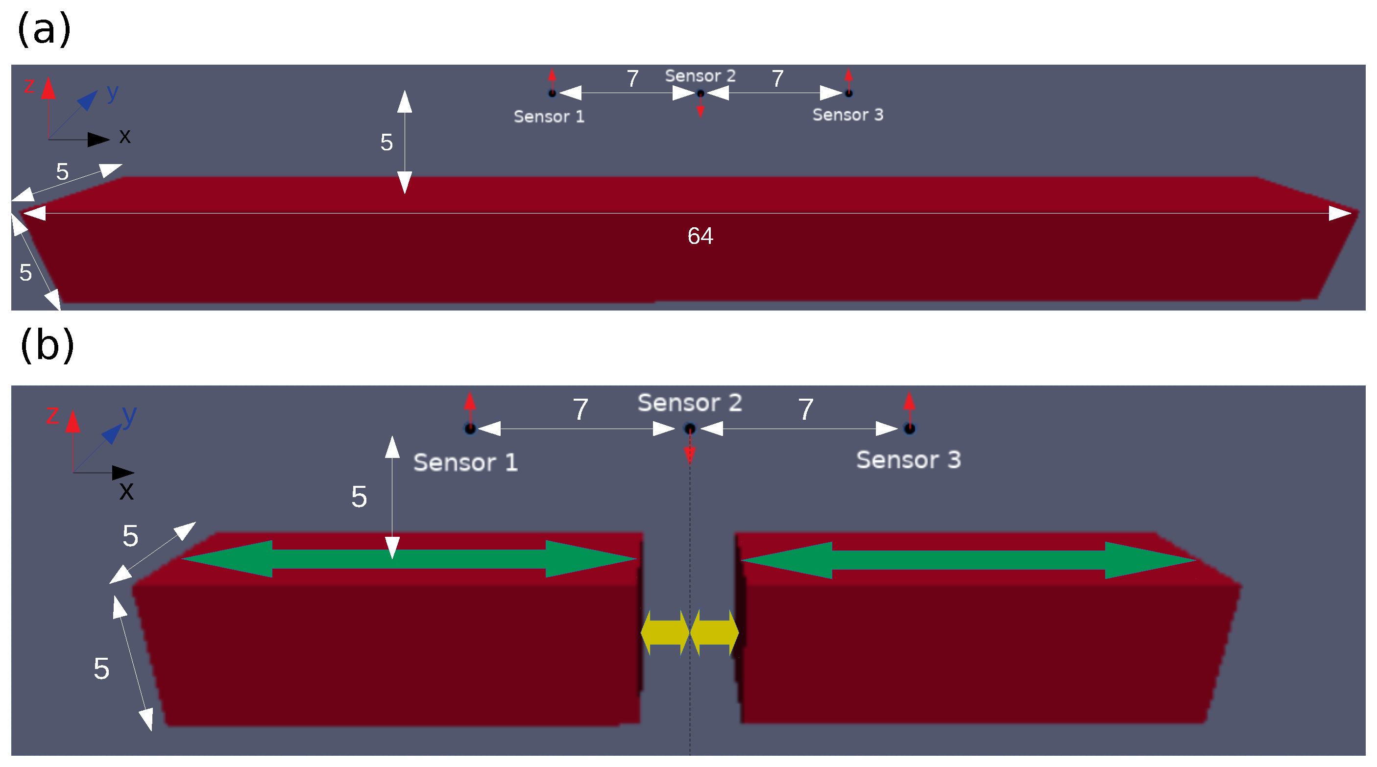
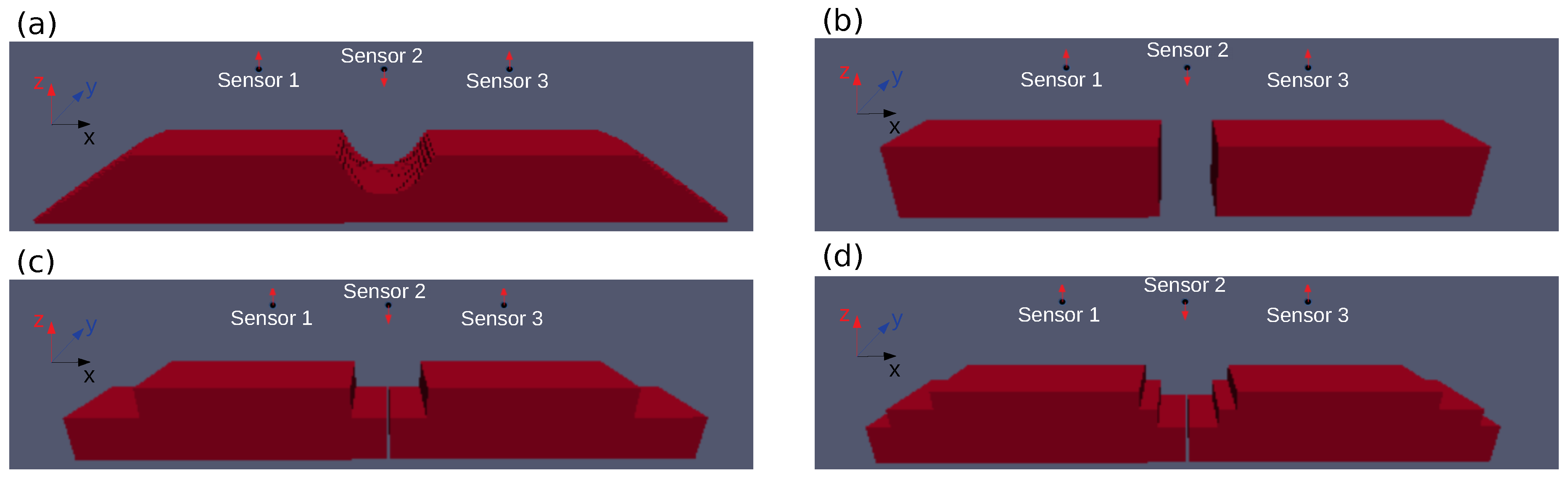
2.2. Field Shaping and Shape Variation

The optimization problem (6) is reminiscent of inverse magnet design for field shaping [24,26]. There is however a crucial difference. While field shaping attempts to give the magnetic field a specific, favorable form (e.g., a linear component [26]) which can then be easily processed for readout, Equation (6) only aims to find the configuration with maximal state separation and relies as such on a more complex form of direct inversion for readout [8]. Field shaping thus requests preliminary knowledge of a target field, whereas the proposed MPO design method circumvents this requirement by simply looking at all possible solutions.

To solve the optimization problem (6), it seems nevertheless reasonable to extend field shaping techniques to MPO design. In this context, topology optimization using the adjoint method is able to address thousands of DoFs and to find optimal magnet forms ab initio [24,30,31,32]. However, remarkable results can already be achieved by variation of simple magnet shapes, as proposed in [26]. Comparison and discussion of the two methods are given in Appendix B.

In this paper, an extended version of the shape variation approach is chosen instead of complex procedures like the adjoint method for several reasons. First, the simple magnet forms are commercially available and cheap, while the slightly better performing but very complex magnet shapes that result from the adjoint method are hard to obtain and expensive in fabrication. In addition, the development effort required by shape variation is relatively small, whereas it can be demanding to formulate the complete MPO problem so that it can be treated with the adjoint method, which requires a priori calculation of an analytical variational derivation of the cost function. Complications may arise, for instance, when non-differentiable functions like $min$ or $max$ are involved.

Finally, it is worth noting that field shaping and the proposed MPO design should not be viewed as opposing strategies but rather as synergetic approaches. Indeed, MPO design by shape variation is limited to fewer DoFs and focuses on answering the question of how to realize a motion, which could, in turn, hint at potential target magnetic field shapes suitable for more sophisticated field shaping methods dealing with more DoFs and complex magnet forms.

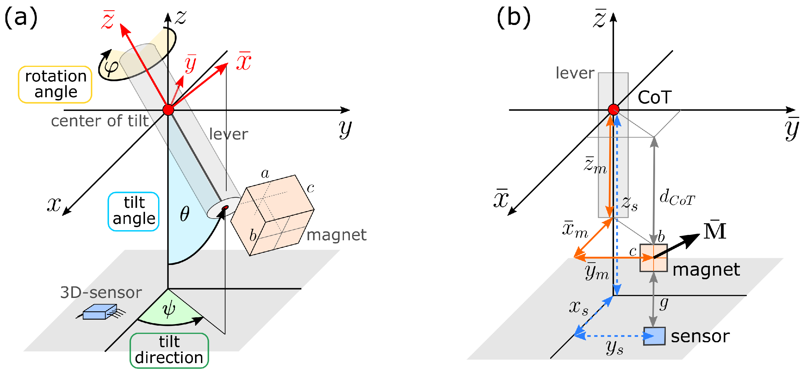
2.3. The Three-Axis Joystick System

Here, the general formalism developed in Section 2.1 is applied to describe a specific MPO system of interest: a three-axis joystick in which the lever can be continuously tilted in two directions and rotated about its own axis. The objective is to resolve this three-axis motion by using only a single magnet and a single 3D magnetic field sensor. Previous works [19,20,21] focused on the extreme cost-efficiency of such an implementation in comparison to state-of-the-art solutions [11,13]. However, they only concentrated on a much simpler implementation with discrete tilt directions and tilt angles.

A convenient representation of the observables of interest describing the three-axis motion is given by the three angles $\psi$, $\theta$, and $\phi$ sketched in Figure 2a: $\psi$ is the azimuth angle corresponding to the lever tilt direction, $\theta$ is the polar angle indicating the amplitude of tilt, and $\phi$ is the rotation angle tracking the lever rotation about its own axis.

According to the general formalism, the observables of interest are thus $\mathit{\alpha }=(\psi ,\theta ,\phi )$. The parameter space P is defined by the corresponding allowed angle ranges, which—consistent with typical three-axis joystick motion—are chosen as $\psi \in {[0,360]}^{\circ }$, $\theta$$\in [0,{\theta }_{\max }]$, and $\phi \in [{\phi }_{\min },{\phi }_{\max }]$.

The MPO system is realized by fixing a permanent magnet at the bottom of the lever and by mounting a 3D magnetic field sensor directly below. This configuration implies that $\mathit{\alpha }$ and the sensor output $\mathbf{B}$ have the same dimension, which reduces the feasibility study to a simpler sign analysis through the use of Equation (2).

The magnet is defined in a local coordinate system (LCS) fixed to the lever which is denoted by barred symbols $\left(\overline{x},\overline{y},\overline{z}\right)$ and coincides with the global coordinates $\left(x,y,z\right)$ when $\mathit{\alpha }=0$. A set of critical system parameters $\mathbf{s}$ is given by the following geometrical and physical quantities:

• the position of a 3D magnetic field sensor ${\mathbf{r}}_s=(x_s,y_s,z_s)$. The sensor output is the magnetic field vector $\mathbf{B}$.
• the magnet position ${\overline{\mathbf{r}}}_m=({\overline{x}}_m,{\overline{y}}_m,{\overline{z}}_m)$ in the LCS. The lengths ${\overline{x}}_m$ and ${\overline{y}}_m$ indicate lateral displacement of the magnet from the lever axis, while ${\overline{z}}_m$ is the distance of the magnet from the center of tilt.
• the magnet magnetization vector $\overline{\mathbf{M}}=({\overline{M}}_x,{\overline{M}}_y,{\overline{M}}_z)$ defined in the LCS, assuming uniform magnetization.
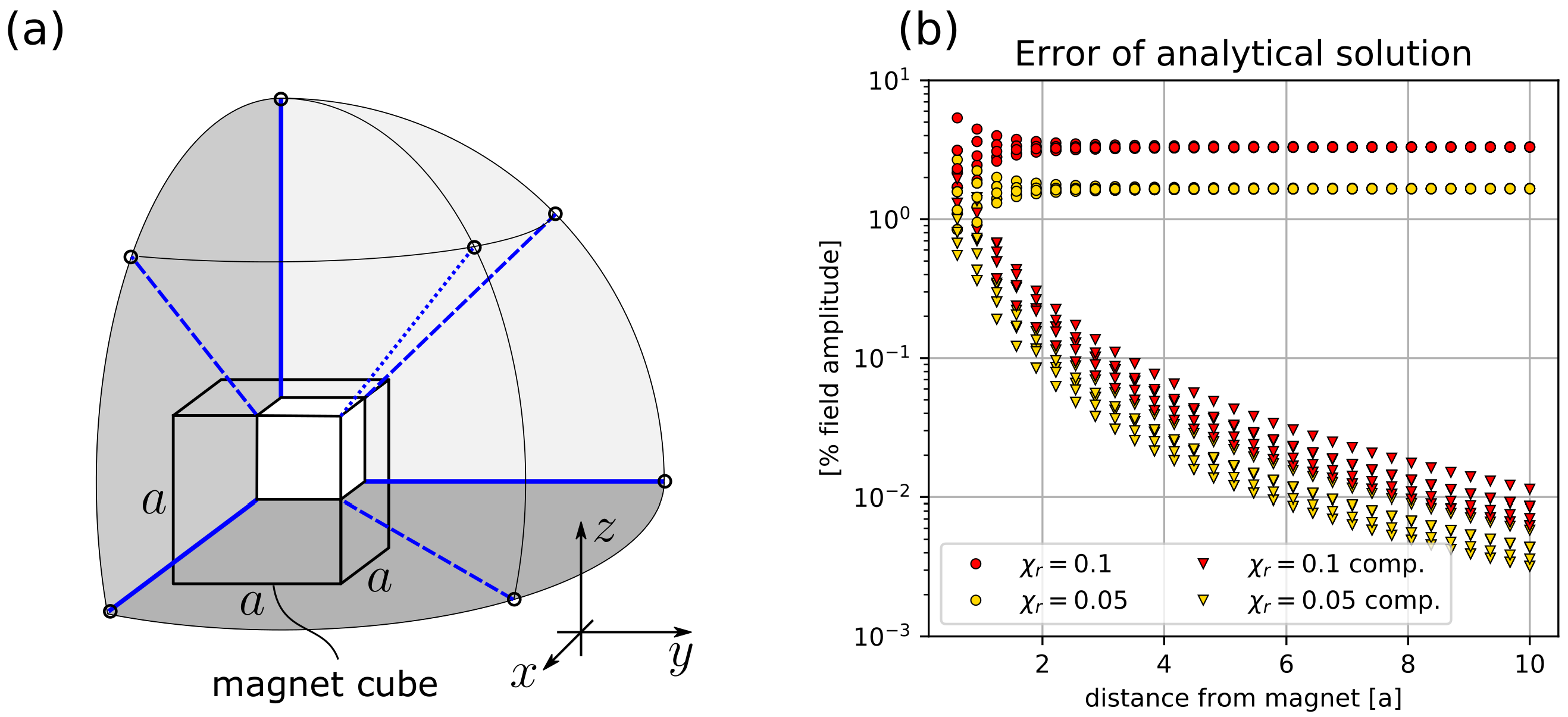
• the size of the magnet given by its side lengths $(a,b,c)$, considering a cuboid magnet shape with orientation ${\overline{\mathbf{e}}}_i^m$ in the LCS. The cuboid magnet shape is chosen for computational reasons; see Section 2.4.

These definitions naturally introduce an additional pair of critical parameters characteristic for such MPO systems, i.e., the airgap $g=z_s-{\overline{z}}_m$ between magnet and sensor as well as the magnet distance from the center of tilt $d_{CoT}={\overline{z}}_m-c/2$. Figure 2a,b shows a schematic of the magnetic joystick with all the corresponding relevant system parameters. The lever, the sensor, and all the other system component materials are chosen to be nonmagnetic (stainless steel, plastics, and silicon). The influences of sensor noise, possible magnetic shielding, external stray fields, or imperfect magnetization are neglected in this study.

The observables of interest $\mathit{\alpha }=(\psi ,\theta ,\phi )$ allow to infer the magnet position ${\mathbf{r}}_m$ and orientation ${\mathbf{e}}_i^m$ in the global coordinate system in terms of a rotation $\mathbf{R}\left(\mathit{\alpha }\right)$ of the magnet position ${\overline{\mathbf{r}}}_m$ and orientations ${\overline{\mathbf{e}}}_i^m$ in the LCS,

$$\begin{array}{cc}\hfill {\mathbf{r}}_m(\mathit{\alpha },\mathbf{s})& =\mathbf{R}\left(\mathit{\alpha }\right){\overline{\mathbf{r}}}_m\left(\mathbf{s}\right),\hfill \end{array}$$

(7)

$$\begin{array}{cc}\hfill {\mathbf{e}}_i^m(\mathit{\alpha },\mathbf{s})& =\mathbf{R}\left(\mathit{\alpha }\right){\overline{\mathbf{e}}}_i^m\left(\mathbf{s}\right).\hfill \end{array}$$

(8)

A derivation of the rotation matrix $\mathbf{R}$ is reported in Appendix C. Assuming that the magnetic field can be computed in the LCS as $\overline{\mathbf{B}}\left(\overline{\mathbf{r}}\right)$, it is possible to determine the sensor output as:

$$\mathbf{B}(\mathit{\alpha },\mathbf{s})=\mathbf{R}\left(\mathit{\alpha }\right)\overline{\mathbf{B}}({\overline{\mathbf{r}}}_m\left(\mathbf{s}\right)-{\mathbf{R}}^{-1}\left(\mathit{\alpha }\right){\mathbf{r}}_s\left(\mathbf{s}\right)).$$

(9)

Equation (9) expresses the sensor output $\mathbf{B}$ in terms of both the observables of interest $\mathit{\alpha }$ and the system parameters $\mathbf{s}$, which forms the basis for a further system analysis starting with Equation (1).

2.4. Magnetic Field Computation

Equation (9) requires the magnetic field $\overline{\mathbf{B}}\left(\overline{\mathbf{r}}\right)$ to be computed in the LCS. To this end, several viable options exist, the most commonly employed one being the FE method, as FE environments are readily available from multiple commercial and noncommercial sources [33,34,35,36], though the long computation times involved make such numerical approaches unpractical for dealing with the global multivariate optimization problem (6) that lies at the core of this paper.

As discussed in Section 2.2, the use of analytical solutions of permanent magnet problems [37,38] is envisaged in this work. Specifically, the field of cuboid magnets can be brought to a closed form [39,40], which enables a specifically fast computation of the sensor output. Moreover, cuboid-shaped magnets are commercially available off-the-shelf and their position and orientation can be defined very precisely when they are integrated into a mechanical setup, as opposed to spherical or cylindrical forms.

For implementation of the analytical formulas, the Magpylib Python package [41] is used, which is specially designed for dealing with MPO systems by integrating complex motions like those expressed by Equations (7)–(9). The analytical formulas are fully tested, vectorized, and optimized to ensure computational efficiency, achieving sub-microsecond computation times for calculation of the sensor output on standard x86 CPUs. In addition, a minimal development effort is required, since Magpylib enables system implementation with only a few lines of code, as demonstrated in Appendix D.

The analytical solution provides an excellent approximation of the magnetic field of realistic modern magnets despite neglecting demagnetization effects. A detailed discussion on the validity of this approximation is provided in Appendix E. In general, the error is less than $1\%$ when ${\mu }_r<1.05$ (realistic for high-grade NdFeB, SmCo, or ferrite materials) and when the distance between sensor and magnet is of the same order or larger than the size of the magnet.

Finally, it must be noted that many MPO systems use soft magnetic materials as magnetic shields, flux guides, and concentrators or shimming elements [1,42]. However, not only can soft magnetic materials not be simulated analytically but also they bring a decisive disadvantage to MPO systems: they generate position-dependent external stray fields that cannot be compensated by differential measurement. The current trend in MPO systems is towards increased stray-field stability [6,43,44], and for this reason, soft magnetic components are generally avoided.

2.5. Optimization Algorithm

Equation (6) describes an optimization problem leading to the best possible MPO system layout ${\mathbf{s}}_{\mathrm{opt}}$ that is subject to the constraints $\mathbf{C}$ and that realizes the parameters of interest $\mathit{\alpha }$. The number of layout parameters and, therefore, the difficulty to solve the problem depend strongly on the complexity of the system. A single cuboid magnet already features 12 DoFs through its position, orientation, magnetization, and dimensions alone. For the typical 10–50 critical DoFs in MPO systems (see also the discussion in Appendix B), the differential evolution (DE) algorithm [45] is an excellent choice to solve such an optimization problem.

DE is a population-based evolutionary algorithm for the optimization of continuous variables in multidimensional spaces. Similar to genetic algorithms, it relies on an iterative process where a population is evolved by mutation, crossover, and selection to improve each generation. In contrast to genetic algorithms, however, DE avoids the harmful effect of mutation by carrying it out before the selection process [46].

The DE algorithm is especially well-suited to the MPO optimization problem (6) for several reasons. Firstly, the objective function is complex and its derivatives cannot be easily calculated, thereby favoring the use of such a black box optimization. Secondly, there can be multiple local optima which require the application of a global treatment. Finally, constraints can be easily included by nature of the algorithm, which adds to every new generation-only-allowed solutions.

DE for magnet shape variation relies heavily on the fast computation times provided by the analytical solutions proposed in Section 2.2 and Section 2.4 due to the large populations required for multivariate global optimization. In terms of computational efficiency, this approach can make optimal use of the computational resources on x86 type processors, as different field evaluations are completely independent of each other. The multiple field evaluations necessary to compute one objective function solution ($\mathit{\alpha }$-grid spanning the space P) can be performed on the single instruction multiple data (SIMD) modules using the vectorized code from Magpylib, while the multiple objective function solutions (different values of $\mathbf{s}$) required for constructing a population can be generated in parallel on separate cores. The SciPy [47] implementation of the DE algorithm provides automated multiprocessing and is used in this paper to perform the optimizations.

A similar computational setup was successfully used in the past for calibration of an MPO system [21]. The proposed implementation allows for reproducible and convergent parameter variations with up to several tens of parameters without resorting to extreme computation resources or distributed computation. A variation involving 20 system parameters and 460 field evaluations in the objective function was performed within 56 minutes and 44 seconds on an Intel^® Xeon^® Scalable Processor “Skylake” Gold 6126 (2.60 GHz, 12-Core Socket 3647, 19.25MB L3 Cache) running on 12 cores and converging within 2365 generations with population sizes of 2000 ($n_{\mathrm{pop}}=100$ in the algorithm). This corresponds to ∼639 field evaluations per millisecond, not counting the algorithm effort.

3. Results

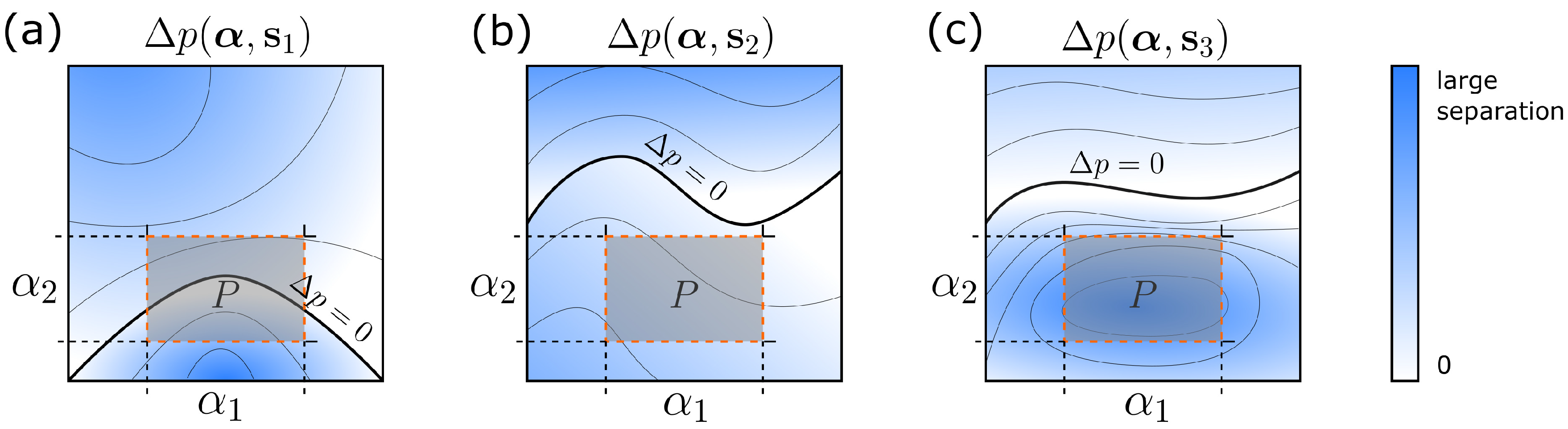
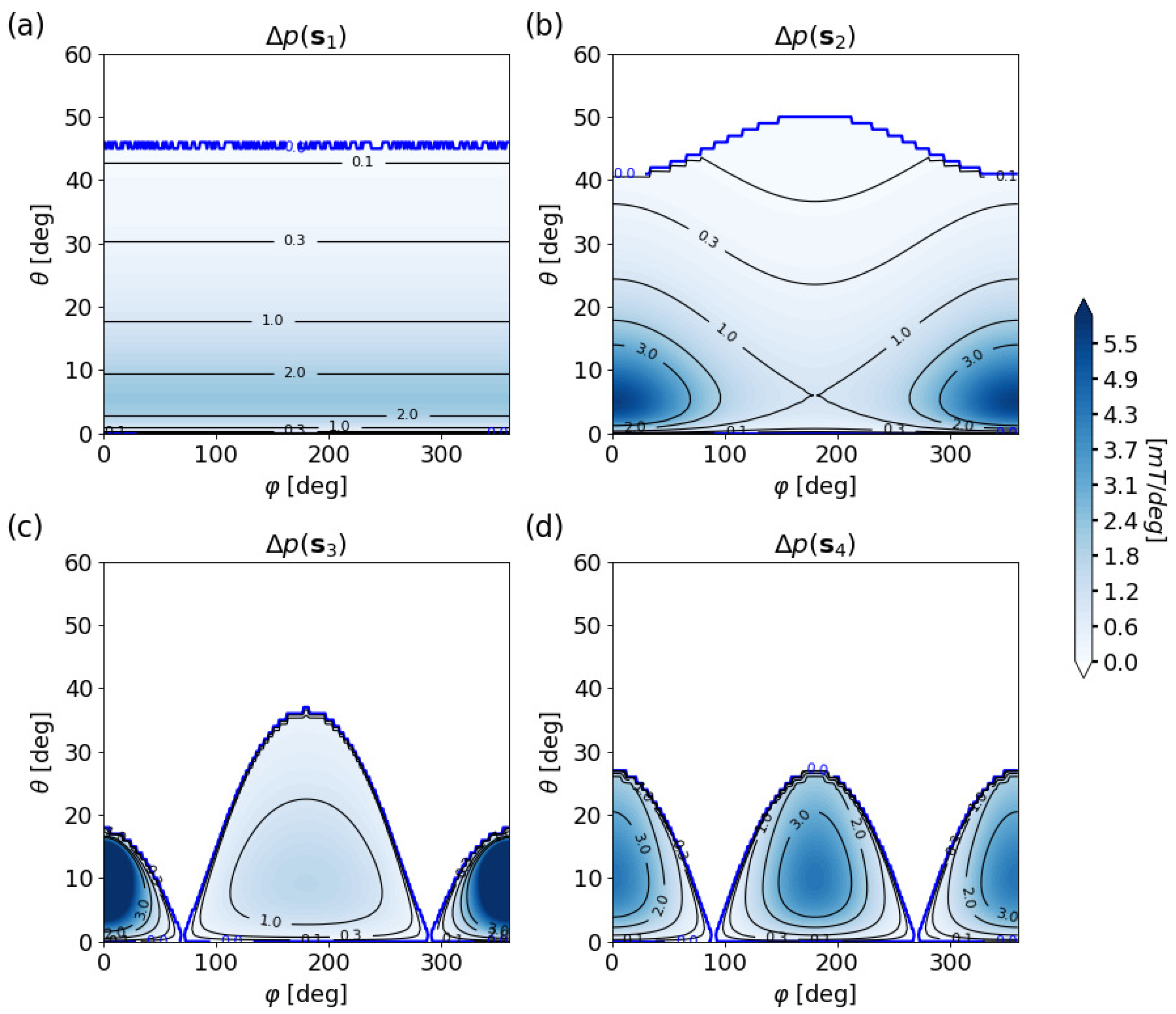
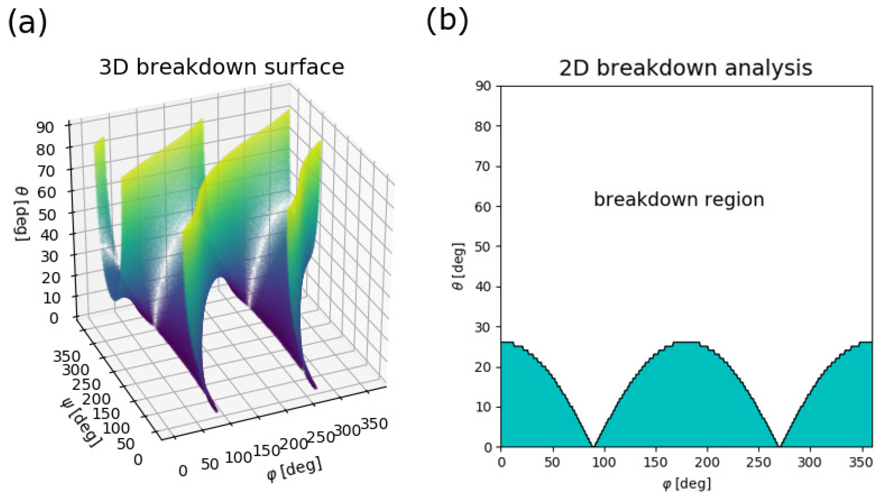
3.1. Feasibility Analysis

A system $\mathbf{s}$ is defined as feasible if it can theoretically solve a given task, i.e., if there is a one-to-one correspondence between the mechanical states of interest $\mathit{\alpha }\in P$ and the sensor output $\mathbf{B}$. Mathematically, this is expressed by Equation (2) for implementation of the three-axis joystick proposed in Section 2.3, where $\mathit{\alpha }$ and $\mathbf{B}$ are of similar dimensions.

A dipole moment is used as a magnetic field source for this feasibility analysis instead of a cuboid magnet. Since the dipole moment is the fundamental entity in magnetism and any magnetization distribution can be constructed from it by superposition, this approach provides a basic physical insight and is easily extended to finite-sized magnets. The magnetic field at the sensor location ${\mathbf{r}}_s$ generated by a dipole moment $\mathbf{m}$ placed at the position ${\mathbf{r}}_m$ is

$$\mathbf{B}(\mathit{\alpha },\mathbf{s})=\frac{{\mu }_0}{4\pi }\left(\frac{3(\mathbf{m}·\mathbf{r})\mathbf{r}}{r^5}-\frac{\mathbf{m}}{r^3}\right),$$

(10)

where $\mathbf{r}(\mathit{\alpha },\mathbf{s})={\mathbf{r}}_s\left(\mathbf{s}\right)-{\mathbf{r}}_m(\mathit{\alpha },\mathbf{s})$ is the distance between the sensor and the magnetic dipole. The position ${\mathbf{r}}_m$ and the orientation of the moment $\mathbf{m}$ are obtained for each mechanical state $\mathit{\alpha }$ through Equations (7) and (8), while the sensor position ${\mathbf{r}}_s$ is fixed completely by the system parameters $\mathbf{s}$.

For a generic implementation, it is always possible to find a connected parameter space P that satisfies (2). One must only make sure that P does not cross a breakdown hypersurface, i.e., surfaces where $\Delta p=0$, as sketched in Figure 1 for two observables. Figure 3a displays such a breakdown surface for a system with ${\overline{\mathbf{r}}}_m=(0,0,0)\mathrm{mm}$, ${\mathbf{r}}_s=(3,0,0)\mathrm{mm}$ and and a magnetic moment ${\mu }_0\overline{\mathbf{m}}=(0,1.25·{10}^5,0)\mathrm{mT}·{\mathrm{mm}}^3$ that corresponds to the magnetic moment of a cube having 5-mm-long sides and a $1000\mathrm{mT}$ remanence field. Any feasible connected parameter space P must lie completely either above or below the breakdown surface. The limited choices for sensing regions for this specific implementation are immediately apparent: it is, for example, possible to realize a system addressing all tilt directions $\psi \in {[0,360]}^{\circ }$, but only when restricting tilt angle $\theta$ and rotation angle $\phi$. The possibility to include all tilt directions can be understood through a projection of the breakdown surface along the $\psi$-direction: the 3D breakdown surface then becomes a 2D breakdown region which is shown in Figure 3b.

For a feasibility analysis including all angles, $\psi ,\phi \in {[0,360]}^{\circ }$, magnet and sensor positions can be reduced to ${\overline{\mathbf{r}}}_m=({\overline{x}}_m,0,{\overline{z}}_m)$ and ${\mathbf{r}}_s=(x_s,0,z_s)$ with ${\overline{x}}_m,x_s\ge 0$ without loss of generality due to the rotation symmetry. Fundamentally different behaviors are observed when the magnet displacement exceeds the sensor displacement (${\overline{x}}_m>x_s$) or when the opposite is the case (${\overline{x}}_m<x_s$). This is demonstrated in Figure 4, where four variations are displayed:

• system type ${\mathbf{s}}_1:$ sensor in the center, magnet displaced ($x_s=0,{\overline{x}}_m>0$),
• system type ${\mathbf{s}}_2:$ sensor and magnet displaced, magnet further out ($x_s<{\overline{x}}_m$),
• system type ${\mathbf{s}}_3:$ sensor and magnet displaced, sensor further out ($x_s>{\overline{x}}_m$),
• system type ${\mathbf{s}}_4:$ magnet in center, sensor displaced ($x_s>0,{\overline{x}}_m=0$).

Systems ${\mathbf{s}}_1$ and ${\mathbf{s}}_4$ are special cases of ${\mathbf{s}}_2$ and ${\mathbf{s}}_3$, respectively, with specific technical relevance.

In Figure 4e–h, the sensing regions for typical representatives of the four cases are shown: ${\mathbf{s}}_1$ with ${\overline{\mathbf{r}}}_m=(3,0,-3)$ and ${\mathbf{r}}_s=(0,0,-6)$; ${\mathbf{s}}_2$ with ${\overline{\mathbf{r}}}_m=(3,0,-3)$ and ${\mathbf{r}}_s=(0.5,0,-6)$; ${\mathbf{s}}_3$ with ${\overline{\mathbf{r}}}_m=(0.5,0,-3)$ and ${\mathbf{r}}_s=(3,0,-6)$; and ${\mathbf{s}}_4$ with ${\overline{\mathbf{r}}}_m=(0,0,-3)$ and ${\mathbf{r}}_s=(3,0,-6)$. For all the systems under investigation, gap and distance from the center of tilt are fixed to $g=3$ and $d_{CoT}=3$, respectively. All the positions are given in units of millimeters. Magnetic moment orientations along the three unit directions are considered for each system: $\overline{\mathbf{m}}\Vert {\overline{\mathbf{e}}}_x$ (black), $\overline{\mathbf{m}}\Vert {\overline{\mathbf{e}}}_y$ (blue), and $\overline{\mathbf{m}}\Vert {\overline{\mathbf{e}}}_z$ (red) with ${\mu }_0\left|\mathbf{m}\right|=1.25·{10}^5\mathrm{mT}·{\mathrm{mm}}^3$.

Figure 4 shows that the shape of the sensing region strongly depends on the implementation $\mathbf{s}$. Specifically, the sensing region becomes maximal in size when the magnetic moment is perpendicular to the plane spanned by the sensor position and the lever axis for $\mathit{\alpha }=0$ (blue sensing regions):

$$\mathbf{m}\perp ({\mathbf{r}}_{\mathbf{s}}\times {\mathbf{e}}_{\mathbf{z}}).$$

(11)

It is interesting to observe that full rotation $\phi \in {[0,360]}^{\circ }$ can only be realized when the magnet displacement exceeds the sensor displacement (${\overline{x}}_m>x_s$) and while the perpendicularity condition (11) is simultaneously fulfilled. At the transition from ${\overline{x}}_m>x_s$ to ${\overline{x}}_m<x_s$ (see Figure 4f,g), the large connected sensing region splits up into two disconnected lobes with opposite signs of the Jacobian determinant.

To better understand the breakdown for different implementations, the magnetic field of the two systems ${\mathbf{s}}_1$ and ${\mathbf{s}}_4$ is displayed in Figure 5. Different colors correspond to different tilt angles. The loops correspond to variations of the tilt direction $\psi \in {[0,360]}^{\circ }$, while the lines connecting different loops are variations of the rotation angle $\phi \in {[0,90]}^{\circ }$. The iso-surfaces of ${\mathbf{s}}_1$ systems are simple toroids, as shown in panel (a), while they cross each other at the transition from sensing region to breakdown region in ${\mathbf{s}}_4$ type systems, which can be observed in panel (b). It is necessary to check if the displayed iso-surfaces form simply connected regions for a valid implementation; see the discussion in Appendix A.

Figure 5a shows that the tilt directions (displayed in steps of ${30}^{\circ }$) are not homogeneously spaced on the loops. For a fixed tilt angle and four fixed tilt directions separated by ${90}^{\circ }$, the rotation angle iso-lines form non-intersecting loops, i.e., circles all passing through each other without intersecting. This forms the basis of the Mini-Drive implementation [19,21], where only 4 discrete tilt directions are considered.

As a result of a systematic investigation, a general empirical rule is proposed to determine the limits of the sensing region for ${\mathbf{s}}_1$ and ${\mathbf{s}}_4$ under the assumption that the perpendicularity condition is fulfilled. The maximum tilt angle ${\theta }_{max}$ can be estimated as

$${\theta }_{\max }\simeq arctan\left(\left|\frac{{\overline{x}}_m}{{\overline{z}}_m}\right|\right)+arctan\left(\left|\frac{x_s}{z_s}\right|\right).$$

(12)

The values of ${\theta }_{\max }$ predicted by means of Equation (12) are reported in Figure 4e,h.

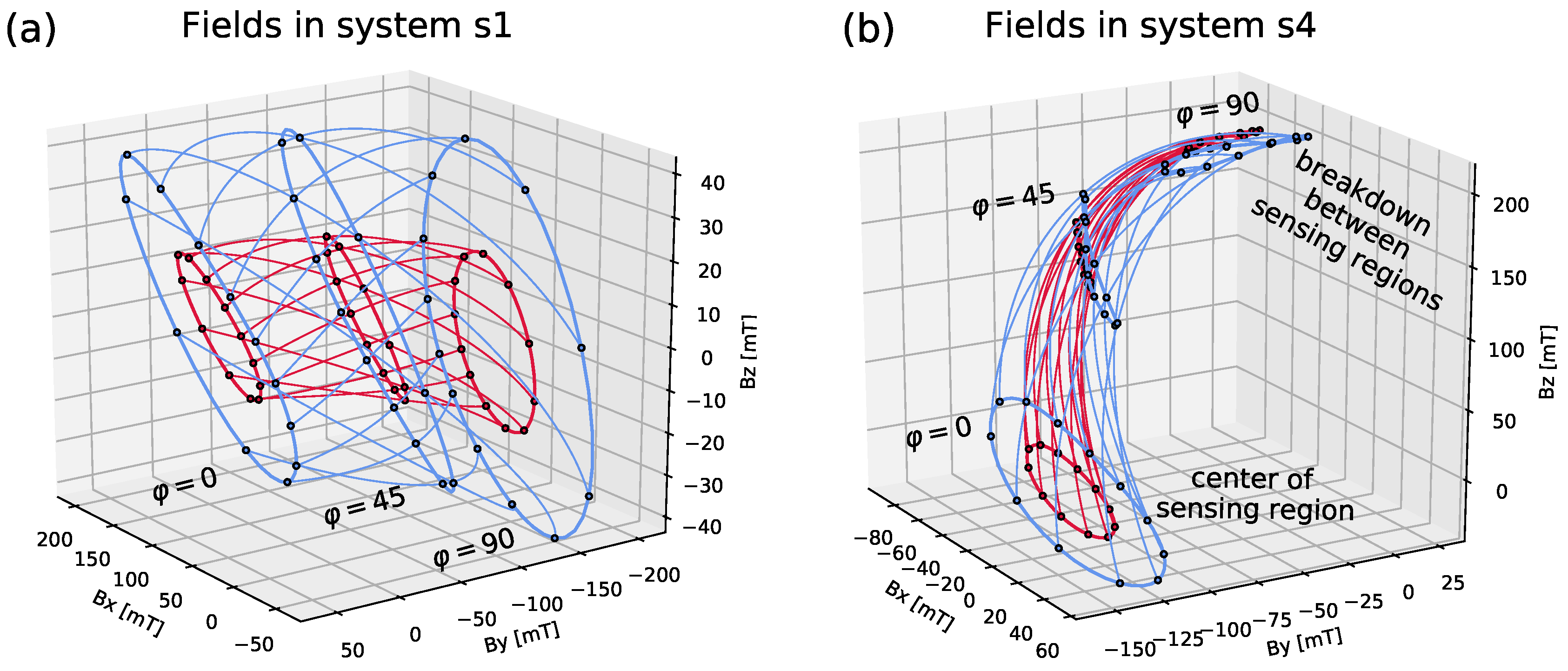
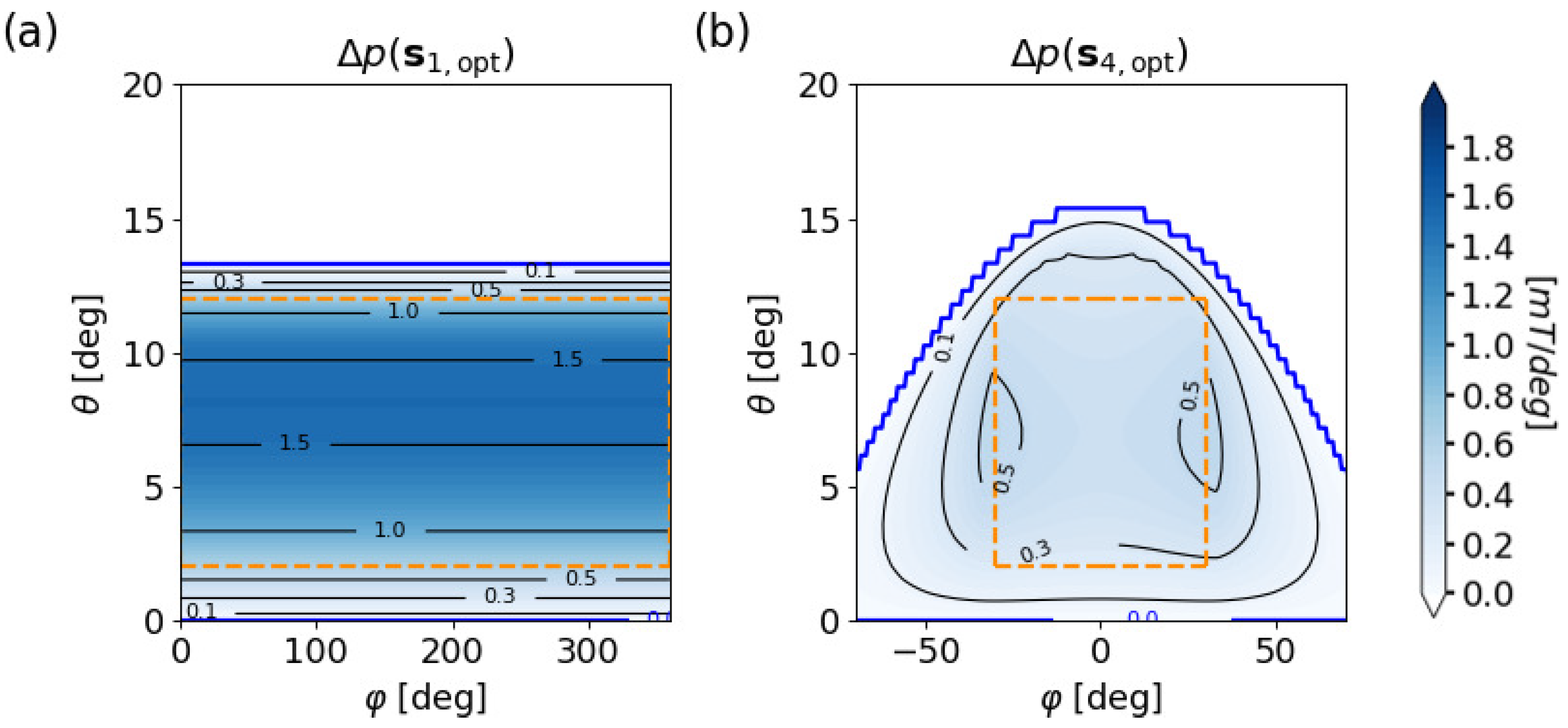
3.2. Quality Analysis

The feasibility analysis specifies which systems are in principle possible but provides no information about the quality, which is expressed in (4) by the DOS and the state separation $\Delta p$. A specific implementation $\mathbf{s}$ is considered to be of high quality when all its mechanical states $\mathit{\alpha }\in P$ are well-separated in magnetic space, as expressed by Equation (5), which ensures easy state identification by the sensor.

For a further analysis of possible implementations, the state separations of the system types ${\mathbf{s}}_1,{\mathbf{s}}_2,{\mathbf{s}}_3,{\mathbf{s}}_4$ defined in Section 3.1 are computed, assuming that the perpendicularity condition (11) is valid. The surprising results are shown in Figure 6a–d, where the sensing region is delimited in blue (in accordance with Figure 4) and the shading corresponds to the state separation.

All systems exhibit low state separations for very small tilt angles. This is the result of the chosen coordinate representation, where the mechanical state density tends to infinity when $\theta \to 0$. However, the singularity is typically avoided by the dead-band ${\theta }_{\mathrm{dead}}$ of several degrees, which typically limits position computation to $\theta >{\theta }_{\mathrm{dead}}$ in most applications [13].

When the sensor lies in the center and the magnet is displaced (system ${\mathbf{s}}_1$), the rotation symmetry makes the DOS independent of the rotation angle $\phi$, which is optimal for the realization of ${360}^{\circ }$ rotation. However, the state separation decays quickly for increasing tilt angles, as the distance between magnet and sensor increases, which makes it difficult to exploit the large ${\theta }_{\max }$ provided by the feasibility study above.

For small sensor displacement, the system makes a transition to ${\mathbf{s}}_2$. The state separation then becomes inhomogeneous in the rotation direction. Rotation angles about $\phi =0^{\circ }$ can be resolved better at the expense of a lower state separation at $\phi ={180}^{\circ }$. This is opposite to the variation of ${\theta }_{\max }$, which becomes smaller around $\phi =0^{\circ }$ but increases at $\phi ={180}^{\circ }$.

When the sensor and magnet are at the same position, there is only a single feasibility lobe with maximum at $\phi ={180}^{\circ }$ and complete breakdown at $\phi =0^{\circ }$. Then, by displacing the sensor beyond the magnet, system ${\mathbf{s}}_3$ is realized. The large central lobe reduces in size and a second small lobe appears at $\phi =0^{\circ }$. Unfortunately, the large lobe—which is good, from a feasibility point of view, for realizing large ranges of the parameters of interest—features a low state separation, while the small lobe exhibits a large one. Both lobes become of equal size with similar state separation when the magnet is located in the center, thereby realizing the system ${\mathbf{s}}_4$.

In summary, an optimal system requires large state separation in the parameter region of interest. Small and inhomogeneous state separations reduce the quality of sensing regions. As shown by the above study, the low quality of the large lobe in ${\mathbf{s}}_3$ and the inhomogeneity of the state separation in system ${\mathbf{s}}_2$ make these implementations inferior in a technical sense to the implementations ${\mathbf{s}}_1$ and ${\mathbf{s}}_4$.

3.3. Optimized Systems with Cuboid Magnets

The two most relevant system types ${\mathbf{s}}_1$ and ${\mathbf{s}}_4$, introduced in Section 3.1, are here optimized in accordance with Equation (6) using the realistic parameters and finite-sized magnets outlined in Section 2.3. The goal of the optimization is to determine the best possible set of realistic system parameters ${\mathbf{s}}_{\mathrm{opt}}$ for given observable ranges of interest.

In both systems, the perpendicularity condition (11) is satisfied, $\overline{\mathbf{M}}=(0,1000,0)\mathrm{mT}$, and an off-the-shelf cubical magnet with $a=b=c=5\mathrm{mm}$ is used. For ${\mathbf{s}}_1$ optimization, the sensor is fixed in the center ($x_s=0\mathrm{mm}$), which results in a state density independent of the rotation angle; see Figure 6a. The parameter space of interest is chosen as $\psi \in {[0,360]}^{\circ }$, $\theta \in {[2,12]}^{\circ }$ and complete rotation $\phi \in {[0,360]}^{\circ }$. For ${\mathbf{s}}_4$ optimization, the magnet is constrained to the center (${\overline{x}}_m=0\mathrm{mm}$) and the parameter space of interest is chosen as $\psi \in {[0,360]}^{\circ }$, $\theta \in {[2,12]}^{\circ }$ and $\phi \in {[-30,30]}^{\circ }$. For both configurations, a common dead-band ${\theta }_{\mathrm{dead}}=2^{\circ }$ is taken into account to avoid the singularity in the state separation at $\theta =0^{\circ }$. Given that most magnetic joystick systems employed in technological applications are millimeter sized, in the optimization procedure, the following reasonable boundaries are used for both the implementations: $g\in [2,4]\mathrm{mm}$ and $d_{\mathrm{CoT}}\in [3,5]\mathrm{mm}$. In addition, the lateral displacements are chosen as ${\overline{x}}_m\in [0.1,15]\mathrm{mm}$ for ${\mathbf{s}}_1$ and $x_s\in [0.1,15]\mathrm{mm}$ for ${\mathbf{s}}_4$.

As expected, for the two optimized systems ${\mathbf{s}}_{1,\mathrm{opt}}$ and ${\mathbf{s}}_{4,\mathrm{opt}}$ the optimization procedure yields the minimum allowed value for the gap $g=2\mathrm{mm}$ and the maximum value of the distance of the magnet from the center of tilt $d_{\mathrm{CoT}}=4.97\mathrm{mm}$: these correspond to small magnet-sensor distances and maximal mechanical state separation. The remaining displacements lead to a maximal state separation when ${\overline{x}}_m=1.52\mathrm{mm}$ and $x_s=3.26\mathrm{mm}$ for ${\mathbf{s}}_{1,\mathrm{opt}}$ and ${\mathbf{s}}_{4,\mathrm{opt}}$, respectively.

Figure 7 displays the state separation $\Delta p$ for the optimal systems.

Panels (a) and (b) show that $\Delta p\left({\mathbf{s}}_{1,\mathrm{opt}}\right)$ is generally larger than $\Delta p\left({\mathbf{s}}_{4,\mathrm{opt}}\right)$ for these implementations with quality factors, computed via Equation (5), of $Q\left({\mathbf{s}}_{1,\mathrm{opt}}\right)=$ 0.64 mT and $Q\left({\mathbf{s}}_{4,\mathrm{opt}}\right)=$ 0.23 mT, respectively. The lower quality of ${\mathbf{s}}_{4,\mathrm{opt}}$ is a result of the much larger lateral displacement which leads to a greater distance between magnet and sensor.

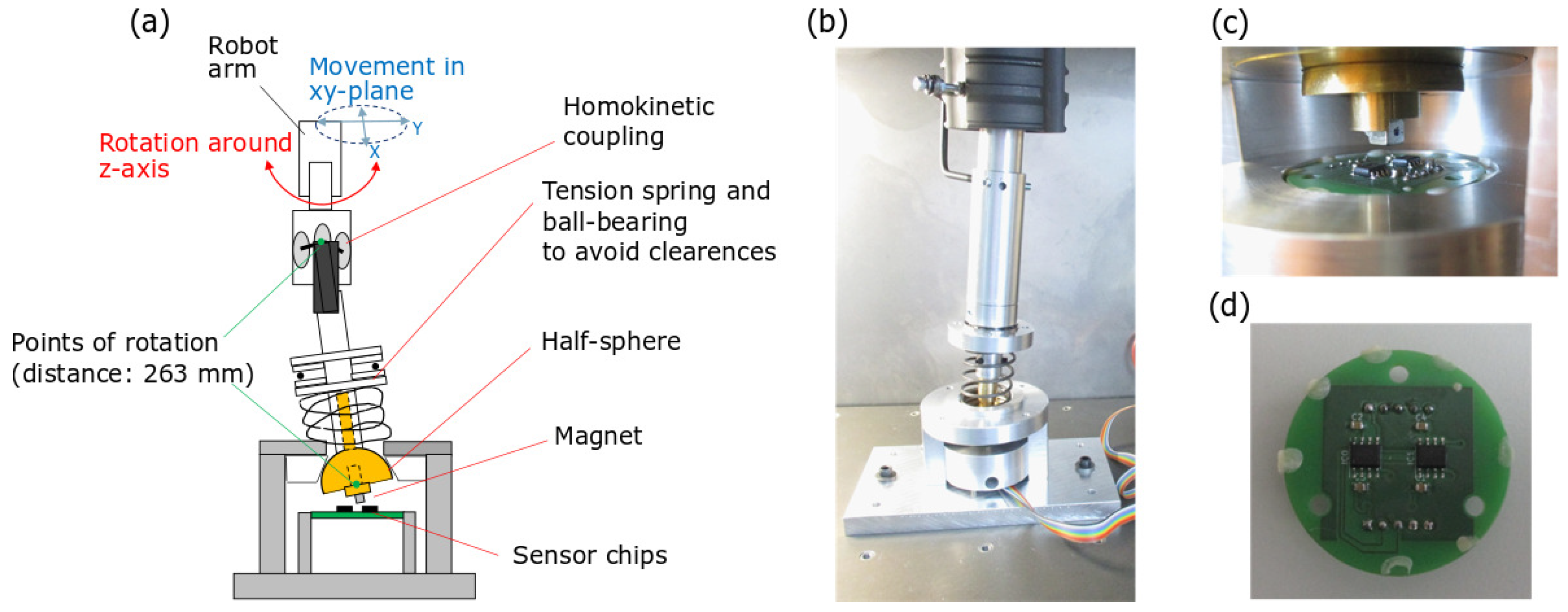
3.4. Experimental Results

In this section, the theoretical predictions are tested in an experiment realizing a system of type ${\mathbf{s}}_4$ with observables of interest $\theta \in {[2,15]}^{\circ }$ and $\phi \in {[-30,30]}^{\circ }$ in accordance with the nautical device presented in [13]. The ${\mathbf{s}}_4$ configuration was chosen because, in contrast to ${\mathbf{s}}_1$ systems, the symmetry allows for integration of two sensors in the same plane (i.e., on a single printed circuit board (PCB)), each one in a different sensing lobe. The second sensor can be used both for redundancy reasons and for the need to compensate external magnetic stray fields by evaluating a differential signal.

The chosen system parameters are the following: a cubical magnet with side length $5\mathrm{mm}$, an airgap of $g=2\mathrm{mm}$, a magnet distance to the center of tilt of $d_{\mathrm{CoT}}=6.83\mathrm{mm}$, and a sensor displacement of $x_s=\pm 5.52\mathrm{mm}$. These parameters are selected as a result of optimization, as outlined in Section 3.3. This optimization includes potential large system fabrication tolerances ($\delta {\overline{x}}_m=\pm 0.5\mathrm{mm}$, $\delta {\overline{y}}_m=\pm 0.5\mathrm{mm}$, $\delta {\overline{z}}_m=\pm 0.5\mathrm{mm}$, $\delta x_s=\pm 0.25\mathrm{mm}$, $\delta y_s=\pm 0.25\mathrm{mm}$, and $\delta g=\pm 0.5\mathrm{mm}$) to ensure reliability and stability of the mechanical system.

The experimental setup is outlined in Figure 8. A custom three-axis joystick is coupled to a robot arm to realize precise mechanical states. The chosen four-axis pick-and-place robot is commonly used to examine linear position and angle sensors. The robot arm is parallel to the z-axis and can move linearly to any point in x-y-z-space with a precision of 30 $\mathsf{\mu }$m. A rotation of the arm around the z-axis is possible with a precision of $0.{02}^{\circ }$. The joystick lever is connected to the robot arm with the help of homokinetic coupling with an integrated length compensation element. This configuration overcomes several difficulties that arise from coupling the linear robot motion to the spherical joystick motion, including a necessary robot arm length compensation, a nonlinear connection between joystick rotation and robot rotation as well as a nonuniform transmission of torque which is not ideal to account for clearances in the setup. Further details on this kind of couplings are reported in [48]. The expected positioning error in this implementation is $0.{01}^{\circ }$ in tilt and $0.{02}^{\circ }$ in rotation when clearances are neglected.

The joystick itself is realized through a center ball (half sphere) which is connected to the rod and pressed into a spherical cavity by two springs and a ball-bearing in order to minimize further clearances in the setup. Figure 8a shows a sketch of the setup, whereas a picture of the actual mechanical realization is displayed in Figure 8b.

The magnet is fixed to the center ball, while two 3D sensors are mounted on a PCB and integrated into the system along the positive and negative directions of the x-axis; see Figure 8c,d. To account for the low state separation, a high-precision 3D Hall sensor with a resolution of $8\mathsf{\mu }\mathrm{T}$ is chosen. The sensor is configured in such way that it provides raw values for the three components of the magnetic flux density.

In the experiment 16,200 mechanical positions are measured in an angle grid with step sizes $\Delta \psi =8^{\circ }$, $\Delta \theta =1^{\circ }$ and $\Delta \phi =2.5^{\circ }$. A comparison between experimental data and theoretical predictions (simulated as discussed in Section 2.4) is shown in Figure 9 for the two sensors at $x_s=5.5\mathrm{mm}$ and $x_s=-5.5\mathrm{mm}$.

The theoretical values show a mean deviation from experimental measurements by 0.1 mT for both the sensors in $x_s=-5.5\mathrm{mm}$ and $x_s=5.5\mathrm{mm}$. The high consistency between theory and experiment is achieved by fitting the theoretical predictions onto the experimental data by variation of 27 tolerances that include sensor position, orientation, gains and offsets, magnet position, orientation, dimensions, magnetization, and experimental angle offsets. All computed tolerances lie within reasonable ranges. The resulting mean angles errors are $\langle e_{\theta }\rangle =0.{067}^{\circ }$, $\langle e_{\phi }\rangle =0.{126}^{\circ }$ and $\langle e_{\psi }\rangle =0.{491}^{\circ }$ and at the 99 percentile, the maximum errors are $e_{\theta ,max}=0.{481}^{\circ }$, $e_{\phi ,max}=0.{658}^{\circ }$ and $e_{\psi ,max}=2.{278}^{\circ }$ for single sensor evaluation. Such errors are at the same level with literature values of 3-DoF and 6-DoF motion tracking [8] where, however, multiple sensors are used for read-out.

4. Conclusions

In this work, the difficulties related to magnet position and orientation (MPO) system design are discussed. A new method for the computation of MPO system layouts is proposed, aimed at maximizing the state separation through a global optimization procedure that is enabled by computationally fast analytical solutions of permanent magnet problems. A comparison to sophisticated topology optimization shows that the proposed computationally inexpensive ansatz can achieve excellent results.

The formalism is applied to study the three-axis-joystick problem. It is shown for the first time that continuous three-axis motion tracking can be realized with only a single magnet and a single 3D magnetic field sensor when fulfilling a specific design criterion that relies on perpendicularity between rotation axis, magnet or sensor displacement, and magnetization direction. For realistic cubical magnets with 5 mm sides and 1000 mT remanence field, a full ${360}^{\circ }$ rotation and tilts up to ${12}^{\circ }$ can be realized at 2 mm airgap with state separation close to 1 mT/${}^{\circ }$. Much larger tilt angles beyond ${60}^{\circ }$ can also be achieved at the expense of state separation. The proposed systems allow for three-axis-joystick motion tracking at unparalleled cost-efficiency. The computations are confirmed by an experimental study where the measured fields are consistent with the theoretical predictions, and resulting mean angle errors are below $0.5^{\circ }$.

This study demonstrates the potential of the proposed formalism in designing novel MPO systems. Future work is dedicated to include system fabrication tolerances in the design process as well as efficient calibration, inversion strategies, and stray field compensation.

References

1. Treutler, C. Magnetic sensors for automotive applications. Sens. Actuators Phys. 2001, 91, 2–6. [Google Scholar] [CrossRef]
2. Granig, W.; Hartmann, S.; Köppl, B. Performance and technology comparison of GMR versus commonly used angle sensor principles for automotive applications. SAE Trans. 2007, 116, 29–41. [Google Scholar]
3. Ortner, M.; Ribeiro, M.; Spitzer, D. Absolute Long-Range Linear Position System With a Single 3-D Magnetic Field Sensor. IEEE Trans. Magn. 2018, 55, 1–4. [Google Scholar] [CrossRef]
4. Hohe, H.; Sauerer, J. Robuste Positionsmessung in Hydraulik-und Pneumatikzylindern. Mechatronik 2008, 11, 60–63. [Google Scholar]
5. Ausserlechner, U. Magnetic Angle Sensors. In Magnetic Sensors and Devices: Technologies and Applications; CRC Press: Boca Raton, FL, USA, 2017; p. 201. [Google Scholar]
6. Huber, S.; Burssens, J.W.; Dupré, N.; Dubrulle, O.; Bidaux, Y.; Close, G.; Schott, C. A gradiometric magnetic sensor system for stray-field-immune rotary position sensing in harsh environment. Multidiscip. Digit. Publ. Inst. Proc. 2018, 2, 809. [Google Scholar] [CrossRef] [Green Version]
7. Bandorf, R.; Ortner, K.; Krau, M. PVD-Abscheidung von CoSm-Schichten für magnetische Maßstäbe: Hohlkathoden-Gasfluss-Sputtern (GFS) für hochwertige Hartmagnetschichten. Vak. Forsch. Und Prax. 2020, 32, 28–32. [Google Scholar] [CrossRef]
8. Cichon, D.; Psiuk, R.; Brauer, H.; Töpfer, H. A Hall-sensor-based localization method with six degrees of freedom using unscented Kalman filter. IEEE Sens. J. 2019, 19, 2509–2516. [Google Scholar] [CrossRef]
9. Popek, K.M.; Schmid, T.; Abbott, J.J. Six-degree-of-freedom localization of an untethered magnetic capsule using a single rotating magnetic dipole. IEEE Robot. Autom. Lett. 2016, 2, 305–312. [Google Scholar] [CrossRef]
10. Infineon Technologies AG, “XENSIV—Sensing the world”, Product catalog, B142-I0675-V2-7600-EU-EC-P. 2020. Available online: https://www.infineon.com/dgdl/Infineon-SensorSelectionGuide-ProductSelectionGuide-v01_00-EN.pdf?fileId=5546d462636cc8fb0164229c09f51bbe (accessed on 30 November 2020).
11. Suchy, J.; Paces, P. BMW iDrive automotive hid device in EFIS control. In Proceedings of the 2014 IEEE/AIAA 33rd Digital Avionics Systems Conference (DASC), Colorado Springs, CO, USA, 5–9 October 2014; p. 2D3-1. [Google Scholar]
12. Danfoss-Heavy-Duty Joysticks. Available online: https://www.danfoss.com/en-us/products/electronic-controls/dps/plus1-joysticks-and-pedals/plus1-joysticks/js1-h/#tab-overview (accessed on 30 November 2020).
13. ZF Products for Marine Propulsion Systems—Joystick Maneuvering System. Available online: https://www.zf.com/products/en/marine/products_29109.html#products_anchor_link_c0150d0cc891-3713-b6e7-018d91295758 (accessed on 30 November 2020).
14. Volvo Penta—Easy Boat Maneuvering. Available online: https://www.volvopenta.com/marine/products/easy-boating-solutions/maneuvering/ (accessed on 30 November 2020).
15. Megatron Precision for Your Design—Joysticks for Industrial and Medical Applications. Available online: https://www.megatron.de/en/category/joysticks.html (accessed on 30 November 2020).
16. Sidestick Airbus Edition. Available online: https://www.thrustmaster.com/en_US/products/tcasidestick-airbus-edition (accessed on 30 November 2020).
17. Arcade Xpress—Mag-Stick. Available online: https://www.arcadexpress.com/en/arcade-joysticks/90-396-joystick-magnetico-industrias-lorenzo.html (accessed on 30 November 2020).
18. Lemken—Joystick Box. Available online: https://lemken.com/en/iqblue/implement-control/auxiliaries/ (accessed on 30 November 2020).
19. Ermakova, A.; Ribeiro, M.; Spitzer, D.; Ortner, M. Analytical Development of a Four-Axis Magnetic Multimedia Control Element. IEEE Sens. J. 2018, 18, 7819–7825. [Google Scholar] [CrossRef]
20. Ortner, M. Magnetic Multimedia Control Element. US Patent 10,048,091, 14 August 2018. [Google Scholar]
21. Lumetti, S.; Malagò, P.; Spitzer, D.; Ortner, M. Computationally efficient calibration of a magnetic position system. Eng. Proc. 2020, 1, 5. [Google Scholar]
22. Infineon TLV493D-A1B6 3D Magnetic Sensor Datasheet. Available online: https://www.infineon.com/dgdl/Infineon-TLV493D-A1B6-DataSheet-v01_10-EN.pdf?fileId=5546d462525dbac40152a6b85c760e80 (accessed on 30 November 2020).
23. Perlepe, P.; Oyarzabal, I.; Mailman, A.; Yquel, M.; Platunov, M.; Dovgaliuk, I.; Rouzières, M.; Négrier, P.; Mondieig, D.; Suturina, E.A.; et al. Metal-organic magnets with large coercivity and ordering temperatures up to 242 °C. Science 2020, 370, 587–592. [Google Scholar] [CrossRef] [PubMed]
24. Bruckner, F.; Abert, C.; Wautischer, G.; Huber, C.; Vogler, C.; Hinze, M.; Suess, D. Solving large-scale inverse magnetostatic problems using the adjoint method. Sci. Rep. 2017, 7, 40816. [Google Scholar] [CrossRef] [PubMed] [Green Version]
25. Balaban, A.L.; Bakhvalov, Y.A.; Denisov, P.A. Review of methods for solving inverse problems in identifying permanent magnets of executive elements in dynamic devices. MATEC Web Conf. 2018, 226, 04022. [Google Scholar] [CrossRef] [Green Version]
26. Ortner, M. Improving magnetic linear position measurement by field shaping. In Proceedings of the 2015 9th International Conference on Sensing Technology (ICST), Auckland, New Zealand, 8–10 December 2015; pp. 359–364. [Google Scholar]
27. Ortner, M.; Huber, C.; Vollert, N.; Pilz, J.; Süss, D. Application of 3D-printed magnets for magnetic position detection systems. In Proceedings of the 2017 IEEE Sensors, Glasgow, UK, 29 October–1 November 2017; pp. 1–3. [Google Scholar]
28. Huber, C.; Abert, C.; Bruckner, F.; Groenefeld, M.; Schuschnigg, S.; Teliban, I.; Vogler, C.; Wautischer, G.; Windl, R.; Suess, D. 3D printing of polymer-bonded rare-earth magnets with a variable magnetic compound fraction for a predefined stray field. Sci. Rep. 2017, 7, 1–8. [Google Scholar] [CrossRef] [Green Version]
29. Gordon, W.B. On the Diffeomorphisms of Euclidean Space. Am. Math. Mon. 1972, 79, 755–759. [Google Scholar] [CrossRef]
30. Abert, C.; Huber, C.; Bruckner, F.; Vogler, C.; Wautischer, G.; Suess, D. A fast finite-difference algorithm for topology optimization of permanent magnets. J. Appl. Phys. 2017, 122, 113904. [Google Scholar] [CrossRef] [Green Version]
31. Huber, C.; Abert, C.; Bruckner, F.; Pfaff, C.; Kriwet, J.; Groenefeld, M.; Teliban, I.; Vogler, C.; Suess, D. Topology optimized and 3D printed polymer-bonded permanent magnets for a predefined external field. J. Appl. Phys. 2017, 122, 053904. [Google Scholar] [CrossRef] [Green Version]
32. Hinze, M.; Pinnau, R.; Ulbrich, M.; Ulbrich, S. Mathematical Modelling: Theory and Applications. In Optimization with PDE Constraints; Springer: New York, NY, USA, 2009; p. xii+270. [Google Scholar]
33. ANSYS Electronics Desktop. Available online: https://www.ansys.com/products/electronics/ansyselectronics-desktop (accessed on 30 November 2020).
34. COMSOL Multiphysics Software. Available online: https://www.comsol.de/ (accessed on 30 November 2020).
35. Abert, C.; Exl, L.; Bruckner, F.; Drews, A.; Suess, D. magnum. fe: A micromagnetic finite-element simulation code based on FEniCS. J. Magn. Magn. Mater. 2013, 345, 29–35. [Google Scholar] [CrossRef] [Green Version]
36. Meeker, D. Finite Element Method Magnetics Software. 2010. Available online: http://www.femm.info/Archives/doc/manual42.pdf (accessed on 30 November 2020).
37. Furlani, E.P. Permanent Magnet and Electromechanical Devices: Materials, Analysis, and Applications; Academic Press: Waltham, MA, USA, 2001. [Google Scholar]
38. Jackson, J.D. Classical Electrodynamics; John Wiley & Sons: New York, NY, USA, 2007. [Google Scholar]
39. Camacho, J.M.; Sosa, V. Alternative method to calculate the magnetic field of permanent magnets with azimuthal symmetry. Rev. Mex. Física 2013, 59, 8–17. [Google Scholar]
40. Yang, Z.; Johansen, T.; Bratsberg, H.; Helgesen, G.; Skjeltorp, A. Potential and force between a magnet and a bulk Y1Ba2Cu3O7-δ superconductor studied by a mechanical pendulum. Supercond. Sci. Technol. 1990, 3, 591. [Google Scholar] [CrossRef]
41. Ortner, M.; Bandeira, L.G.C. Magpylib: A free Python package for magnetic field computation. SoftwareX 2020, 11, 100466. [Google Scholar] [CrossRef]
42. Huber, C.; Goertler, M.; Abert, C.; Bruckner, F.; Groenefeld, M.; Teliban, I.; Suess, D. Additive manufactured and topology optimized passive shimming elements for permanent magnetic systems. Sci. Rep. 2018, 8, 1–8. [Google Scholar] [CrossRef] [PubMed] [Green Version]
43. Dupré, N.; Dubrulle, O.; Huber, S.; Burssens, J.W.; Schott, C.; Close, G. Experimental demonstration of stray-field immunity beyond 5 mt for an automotive-grade rotary position sensor. Multidiscip. Digit. Publ. Inst. Proc. 2018, 2, 763. [Google Scholar] [CrossRef] [Green Version]
44. Grambichler, K.; Binder, G.; Hainz, S.; Köck, H. GMR-basierter, störfeldrobuster Kurbelwellensensor für Hybridfahrzeuge. In Automobil-Sensorik 2; Springer: Berlin, Germany, 2018; pp. 177–198. [Google Scholar]
45. Storn, R. On the usage of differential evolution for function optimization. In Proceedings of the North American Fuzzy Information Processing, Berkeley, CA, USA, 19–22 June 1996; pp. 519–523. [Google Scholar]
46. Rocca, P.; Oliveri, G.; Massa, A. Differential evolution as applied to electromagnetics. IEEE Antennas Propag. Mag. 2011, 53, 38–49. [Google Scholar] [CrossRef]
47. Virtanen, P.; Gommers, R.; Oliphant, T.E.; Haberland, M.; Reddy, T.; Cournapeau, D.; Burovski, E.; Peterson, P.; Weckesser, W.; Bright, J.; et al. SciPy 1.0–Fundamental Algorithms for Scientific Computing in Python. arXiv 2019, arXiv:1907.10121. [Google Scholar] [CrossRef] [Green Version]
48. Farhadi Machekposhti, D.; Tolou, N.; Herder, J. A review on compliant joints and rigid-body constant velocity universal joints toward the design of compliant homokinetic couplings. J. Mech. Des. 2015, 137, 032301. [Google Scholar] [CrossRef]
49. Okamoto, Y.; Takahashi, N. A Novel Topology Optimization of Nonlinear Magnetic Circuit Using ON/OFF Method. IEEJ Trans. Fundam. Mater. 2005, 125, 549–553. [Google Scholar] [CrossRef]
50. Nielsen, K.K.; Bjørk, R. The magnetic field from a homogeneously magnetized cylindrical tile. J. Magn. Magn. Mater. 2020, 507, 166799. [Google Scholar] [CrossRef]
51. Caciagli, A.; Baars, R.J.; Philipse, A.P.; Kuipers, B.W. Exact expression for the magnetic field of a finite cylinder with arbitrary uniform magnetization. J. Magn. Magn. Mater. 2018, 456, 423–432. [Google Scholar] [CrossRef]
52. Rubeck, C.; Yonnet, J.P.; Allag, H.; Delinchant, B.; Chadebec, O. Analytical calculation of magnet systems: Magnetic field created by charged triangles and polyhedra. IEEE Trans. Magn. 2012, 49, 144–147. [Google Scholar] [CrossRef]
53. Hirosawa, S.; Nishino, M.; Miyashita, S. Perspectives for high-performance permanent magnets: Applications, coercivity, and new materials. Adv. Nat. Sci. Nanosci. Nanotechnol. 2017, 8, 013002. [Google Scholar] [CrossRef] [Green Version]
54. Chadebec, O.; Coulomb, J.L.; Janet, F. A review of magnetostatic moment method. IEEE Trans. Magn. 2006, 42, 515–520. [Google Scholar] [CrossRef] [Green Version]
55. Aharoni, A. Demagnetizing factors for rectangular ferromagnetic prisms. J. Appl. Phys. 1998, 83, 3432–3434. [Google Scholar] [CrossRef]
Figure 1. Schematic illustration of the state separation Δ p as a function of the observables of interest α P for 3 different implementations: (a) System s 1 violates the feasibility criterion expressed by Equation (3). (b) System s 2 is a feasible implementation but with bad state separation. (c) System s 3 represents an optimal implementation that not only is feasible but also exhibits a large state separation.
Sensors 20 06873 g001
Figure 2. (a) Illustration of the magnetic joystick system with all its relevant components: the observables of interest are the three angles ψ , θ , and φ describing the joystick motion. The local coordinate system (red axes), fixed to the lever, is denoted by barred variables. (b) Sketch of the critical system parameters.
Sensors 20 06873 g002
Figure 3. (a) Three-dimensional breakdown surface: the color code corresponds to the θ value purely for visualization. (b) Projection along the tilt direction ψ results in a 2D breakdown region and a sensing region (teal), where all ψ [ 0 , 360 ] can be detected.
Sensors 20 06873 g003
Figure 4. Sketches of magnetic joysticks together with the corresponding sensing regions: (ad) geometric representations of implementations s 1 , s 2 , s 3 , and s 4 , respectively, and (eh) the corresponding sensing regions. Black lines and grey regions are for m ¯ e x , blue is for m ¯ e y , and red is for m ¯ e z .
Sensors 20 06873 g004
Figure 5. Magnetic field for the systems (a) s 1 and (b) s 4 illustrated in Figure 4: the fields are displayed for tilt angles θ = 4 (red) and θ = 8 (blue) for rotation angles φ [ 0 , 90 ] and for 12 discrete tilt directions ranging from ψ = 0 to 360 in steps of 30 .
Sensors 20 06873 g005
Figure 6. (ad) State separation Δ p for the four different implementations s 1 to s 4 with m ¯ e ¯ y : the thick blue contour delimits the sensing region.
Sensors 20 06873 g006
Figure 7. State separation Δ p of the optimized systems (a) s 1 , opt and (b) s 4 , opt with m ¯ e ¯ y . Orange dashed lines outline the parameter space α .
Sensors 20 06873 g007
Figure 8. Experimental setup: (a) schematic of the setup; (b) photo of the mechanical setup; (c) zoom-in on the center ball, magnet, and PCB with sensors; and (d) top view of the PCB.
Sensors 20 06873 g008
Figure 9. Comparison between experimental measurements (red dots) and analytical calculation (black lines) in an s 4 -type system with two sensors located at x s = 5.5 mm (a) and x s = 5.5 mm (b), respectively.
Sensors 20 06873 g009
Publisher’s Note: MDPI stays neutral with regard to jurisdictional claims in published maps and institutional affiliations.