First-Order Linear Mechatronics Model for Closed-Loop MEMS Disk Resonator Gyroscope


Abstract
:1. Introduction
2. MEMS DRG and the Configurable ASIC
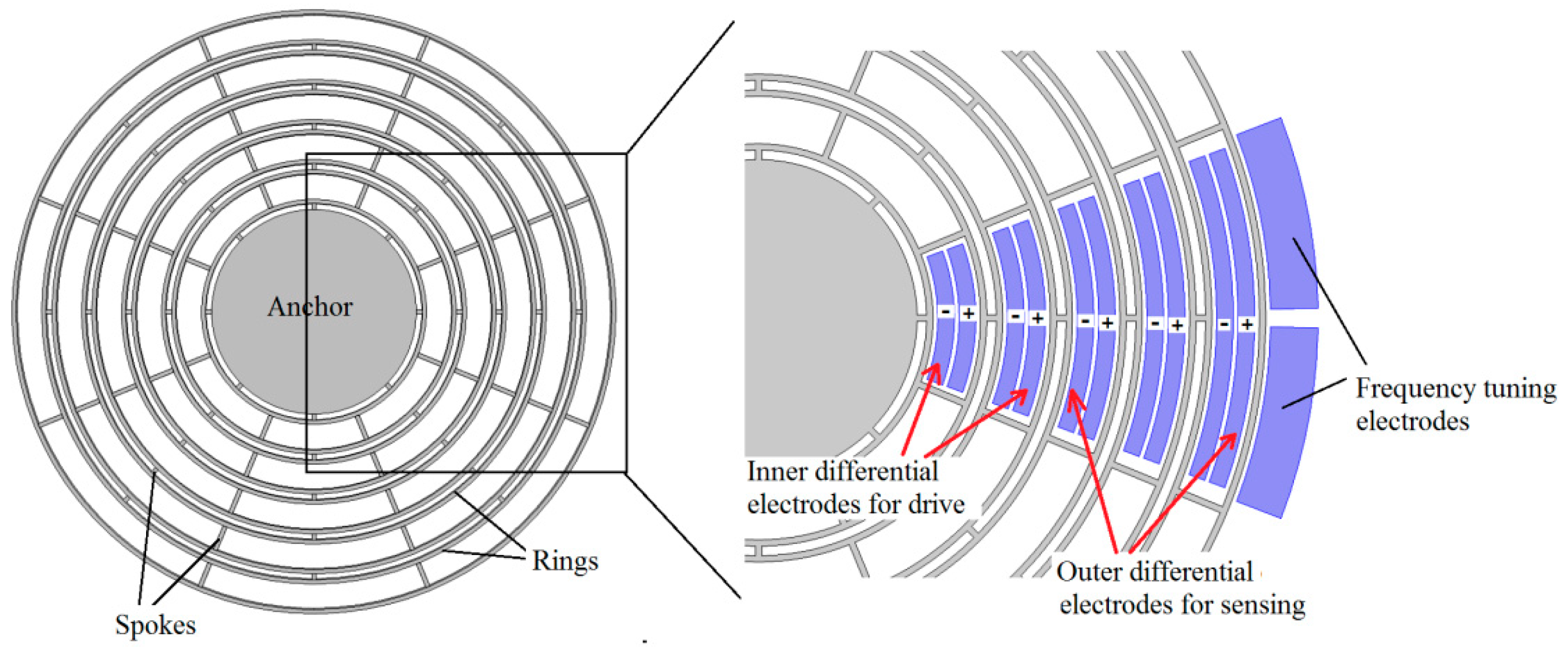
2.1. MEMS Disk Resonator
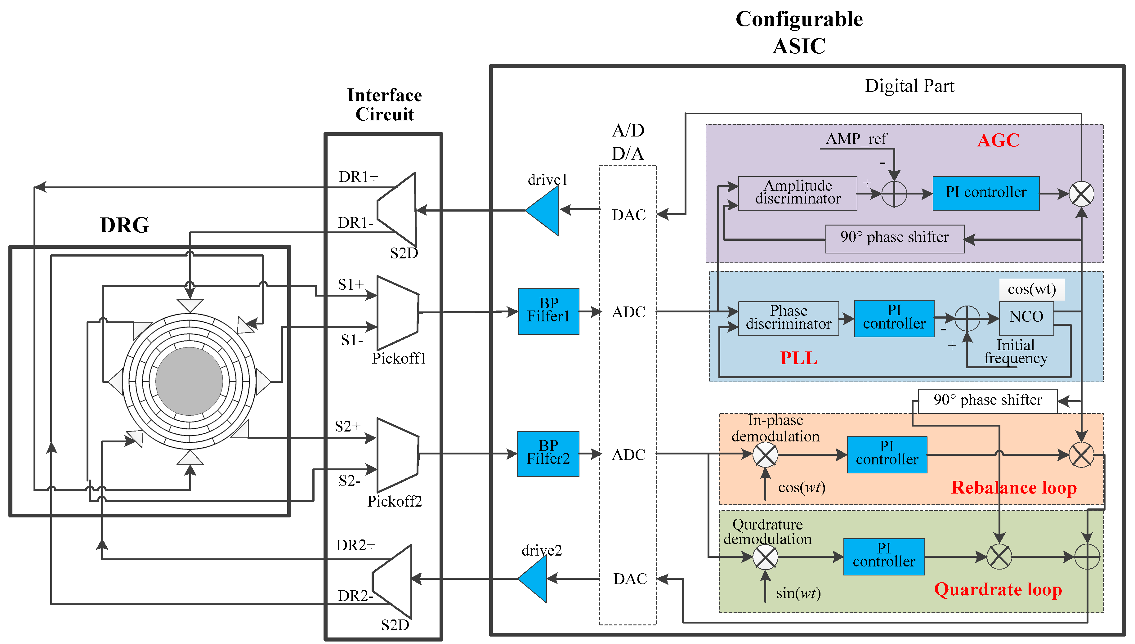
2.2. A Configurable Closed-Loop ASIC for MEMS DRG
- (1)
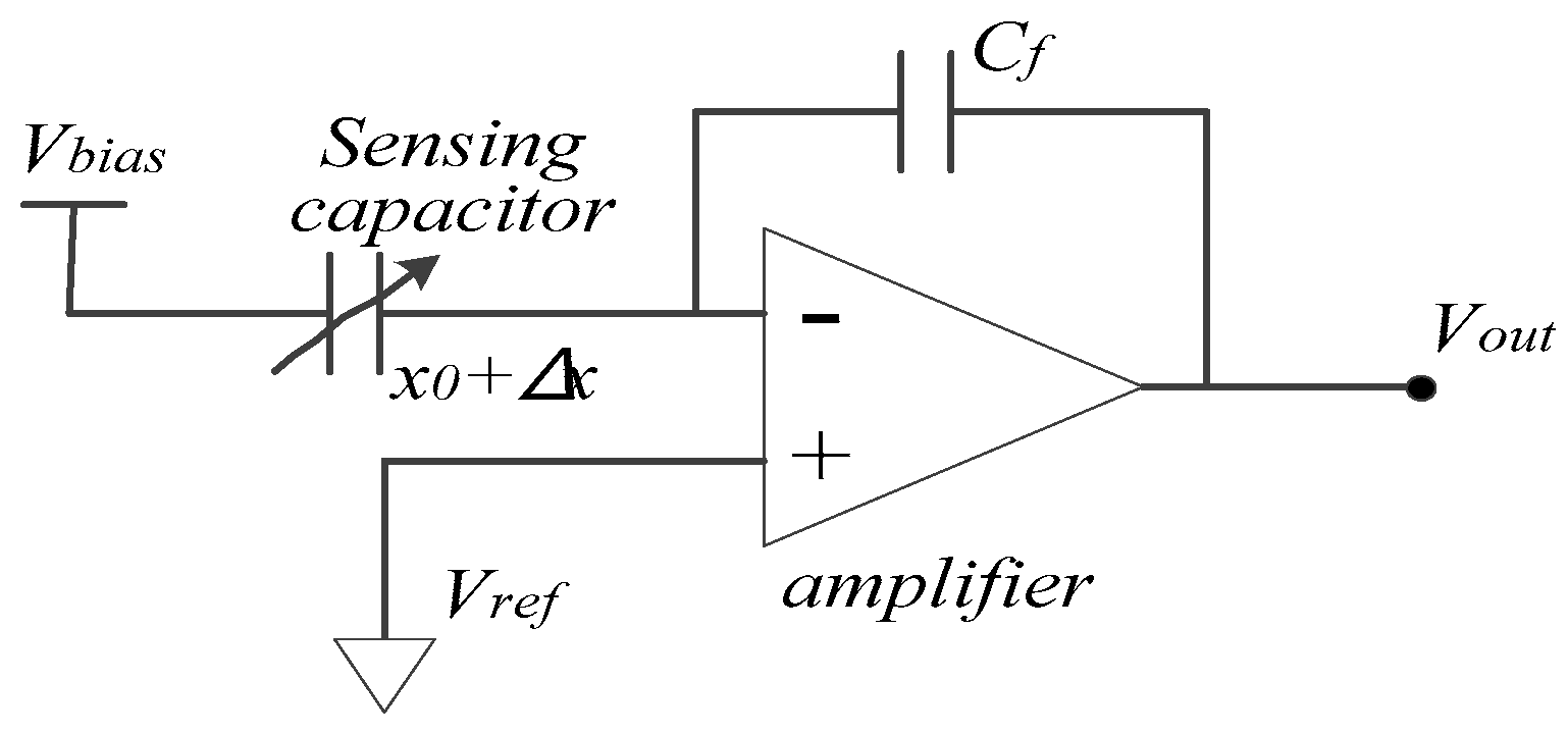
- Pickoff circuit
- (2)
- Analog band-pass filterPickoff circuit
- (3)
- ADCs and DACs
- (4)
- Drive circuit
- (5)
- Digital circuit
- (6)
- Gain of electrostatic feedback force
- (7)
- Gain of Coriolis force
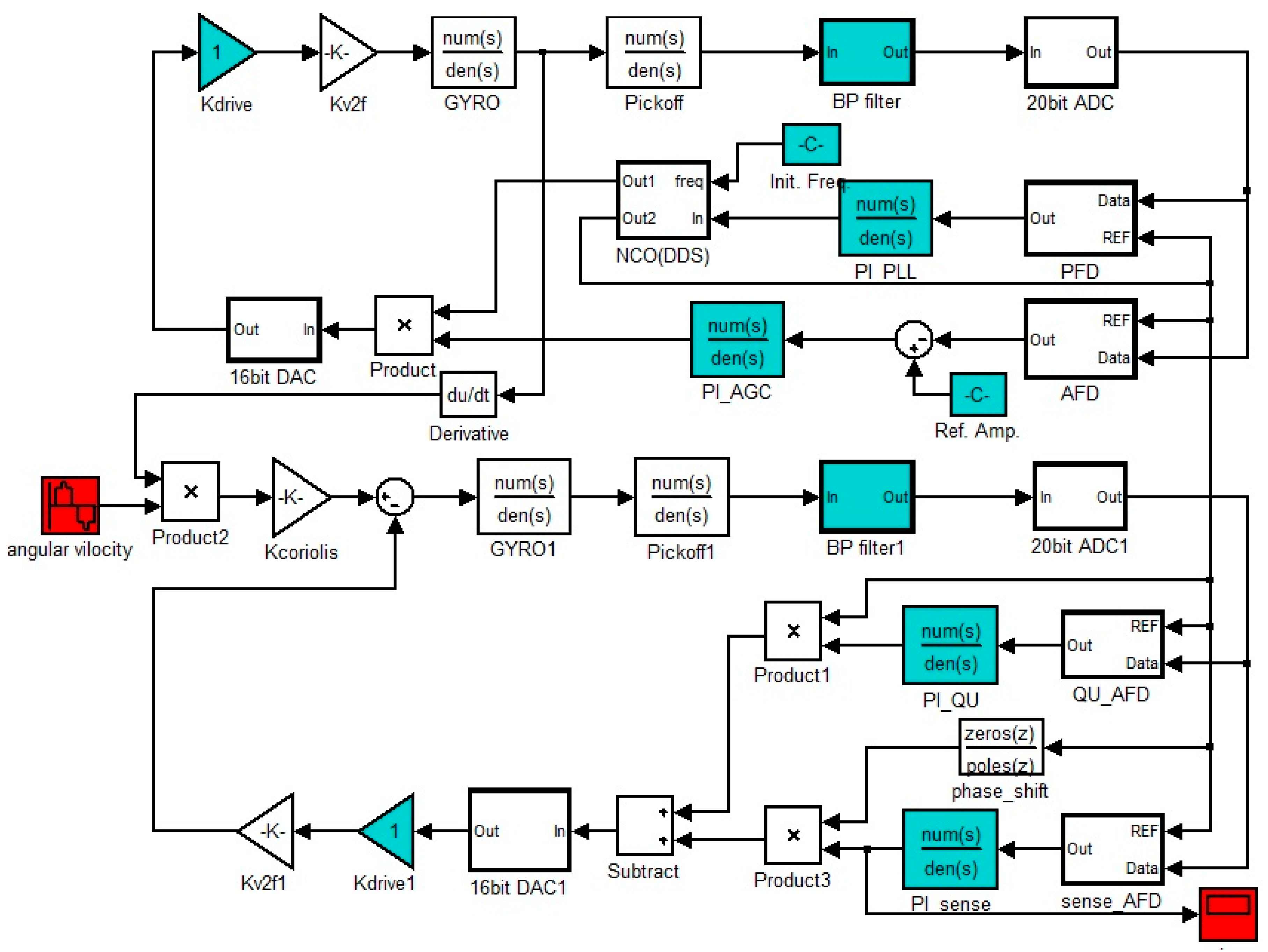
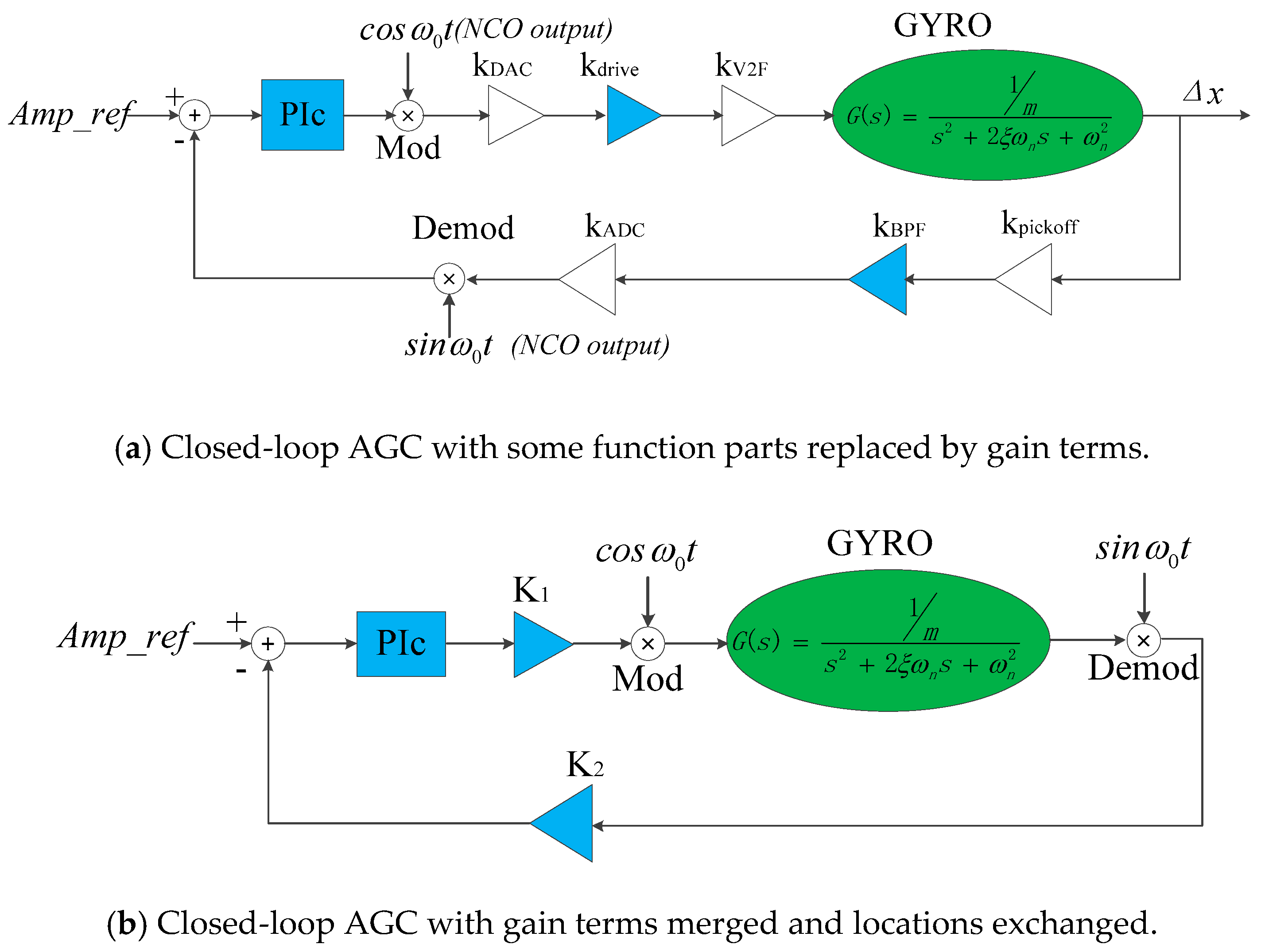
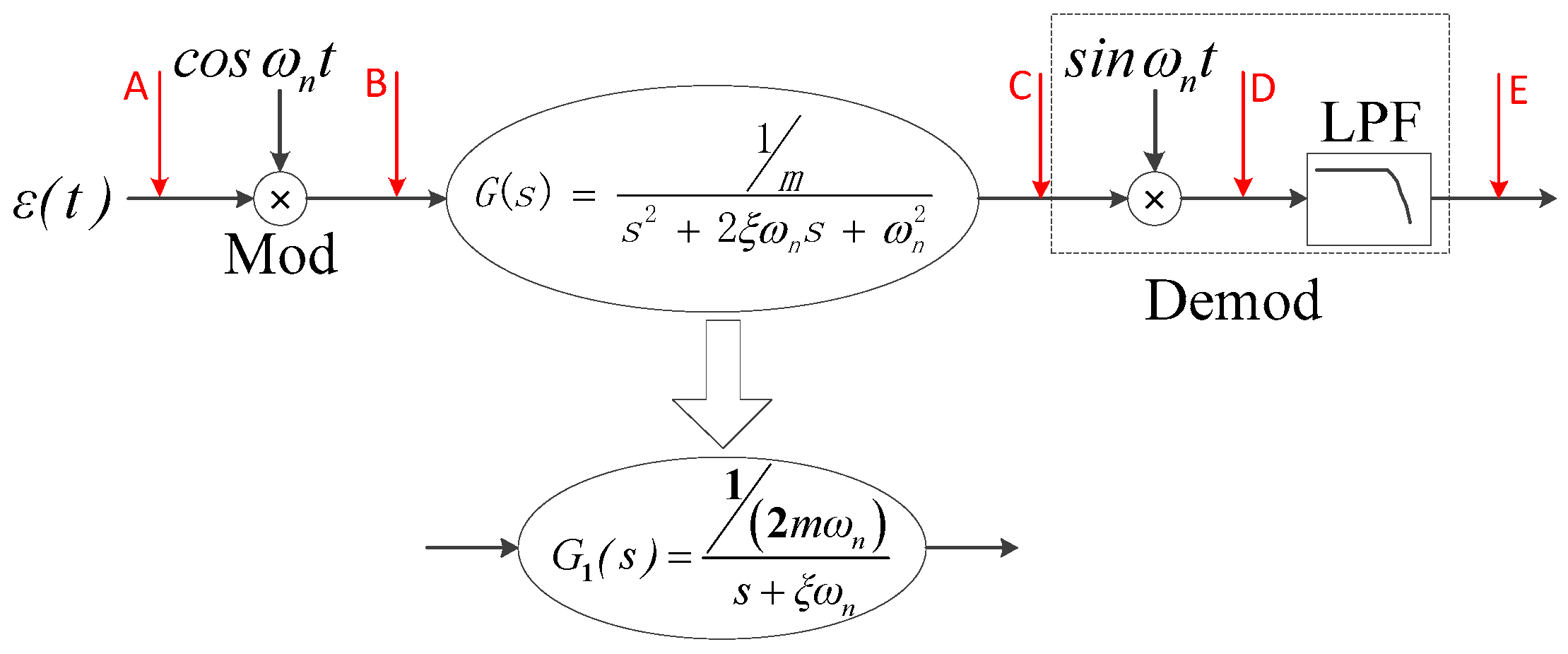
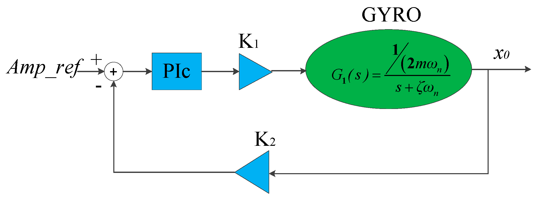
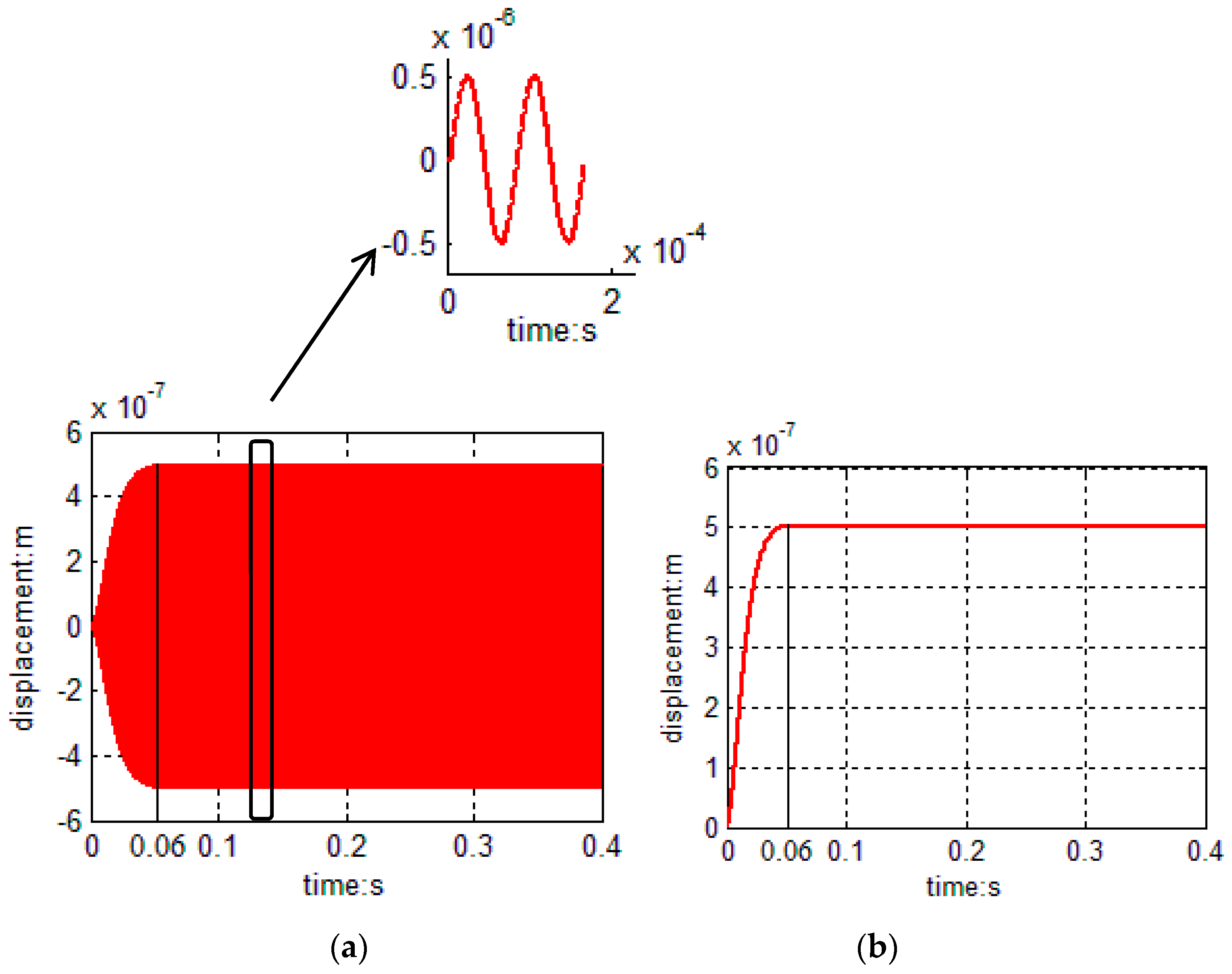
3. Model Linearizing and PI Controllers’ Design for Primary Mode
3.1. AGC Loop Model Order-Reduction and Closed-Loop Design
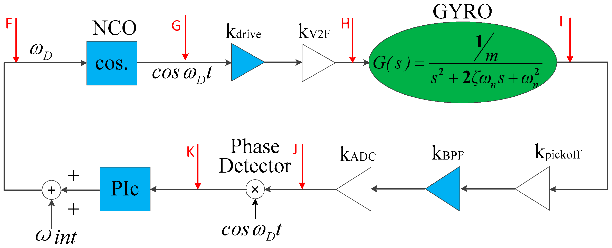
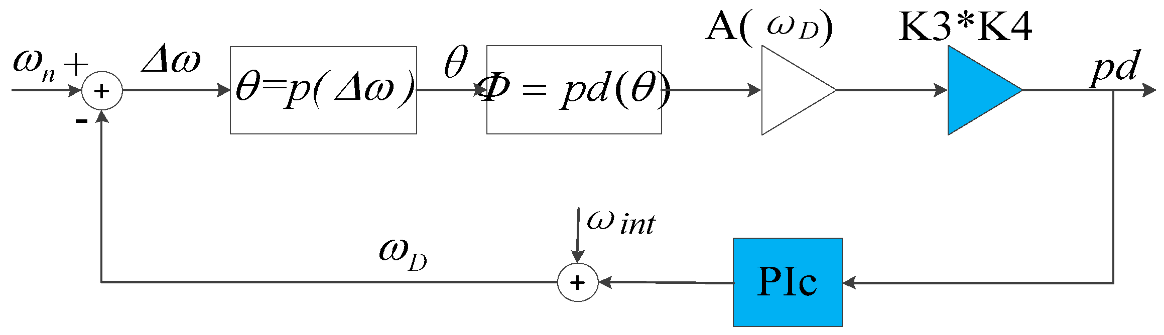
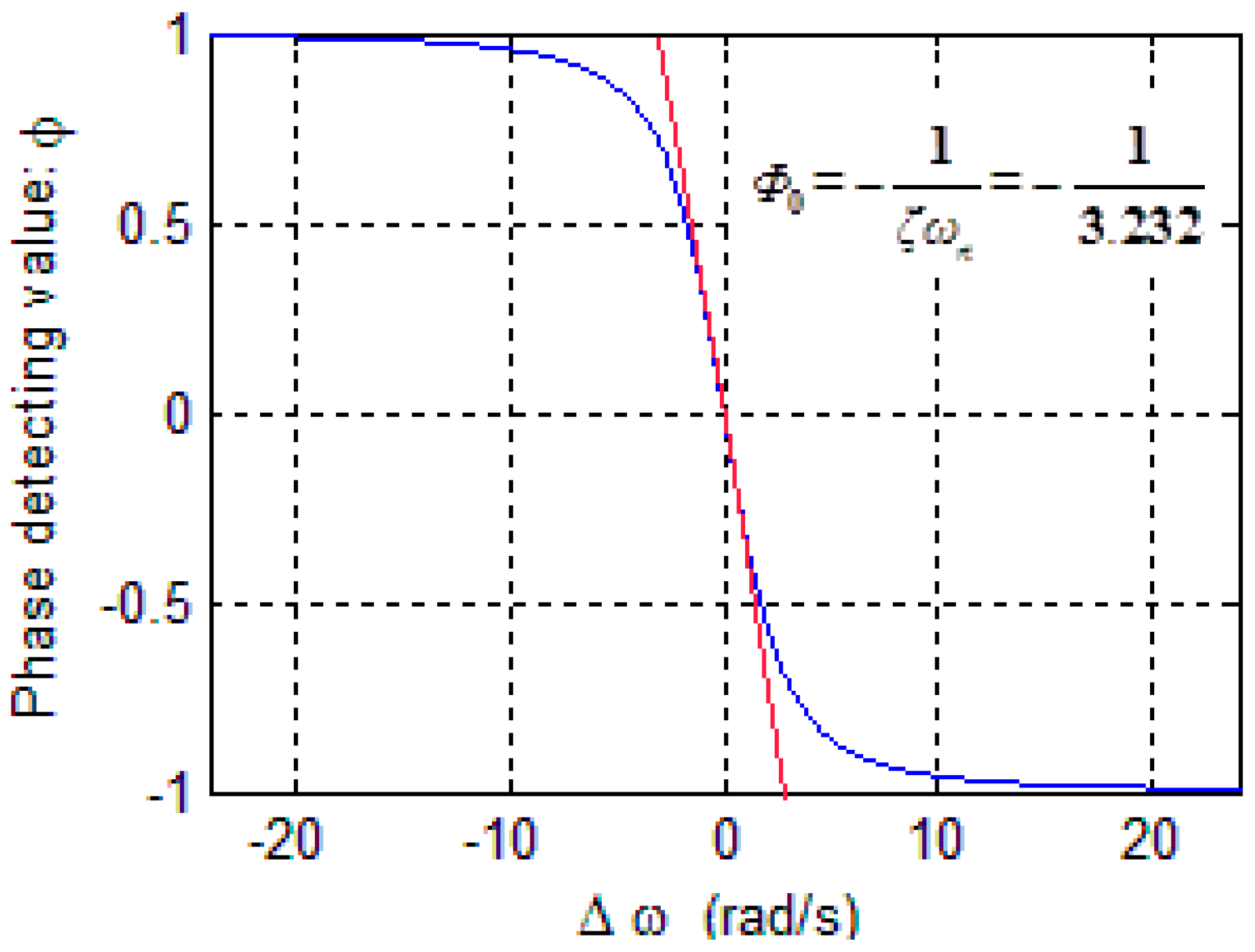
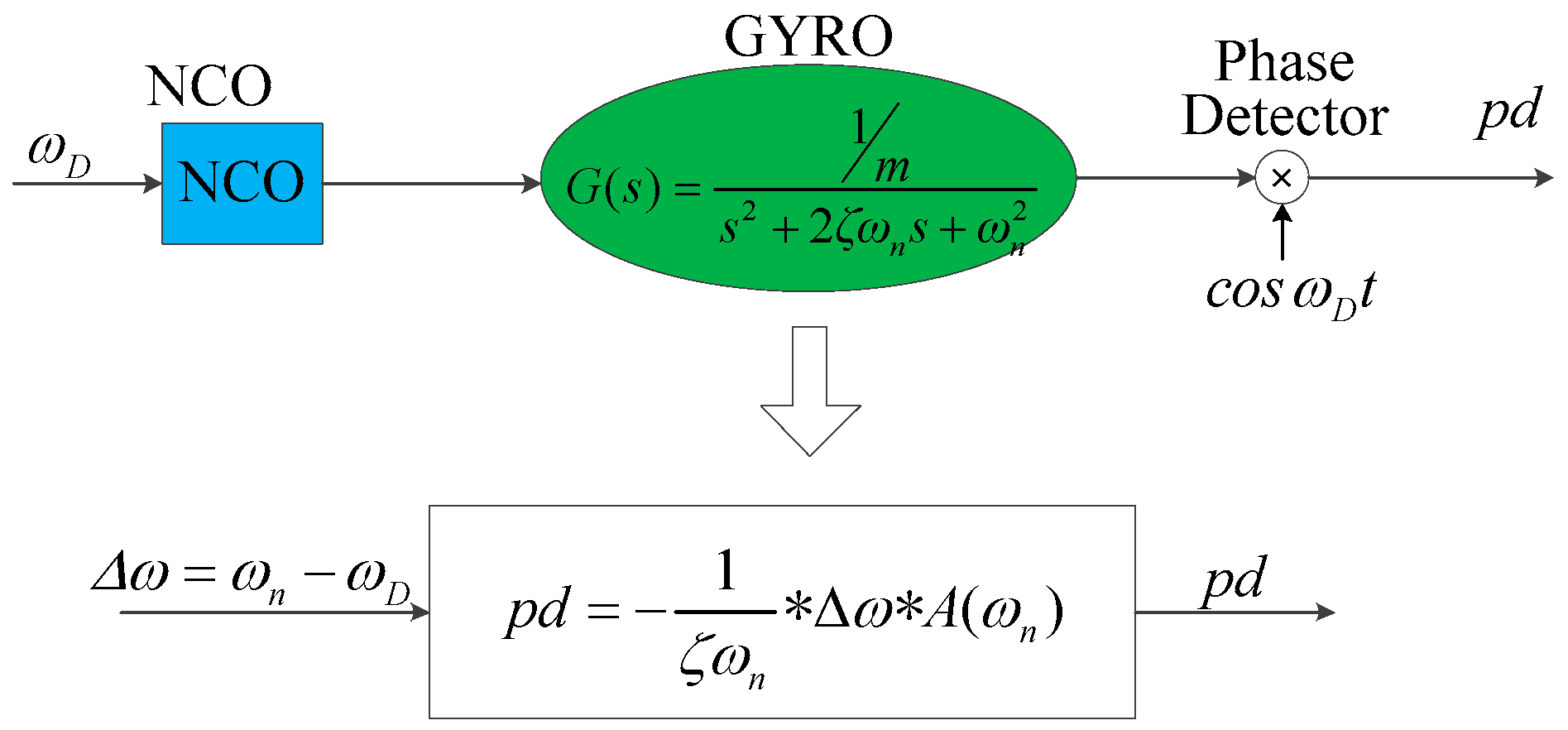
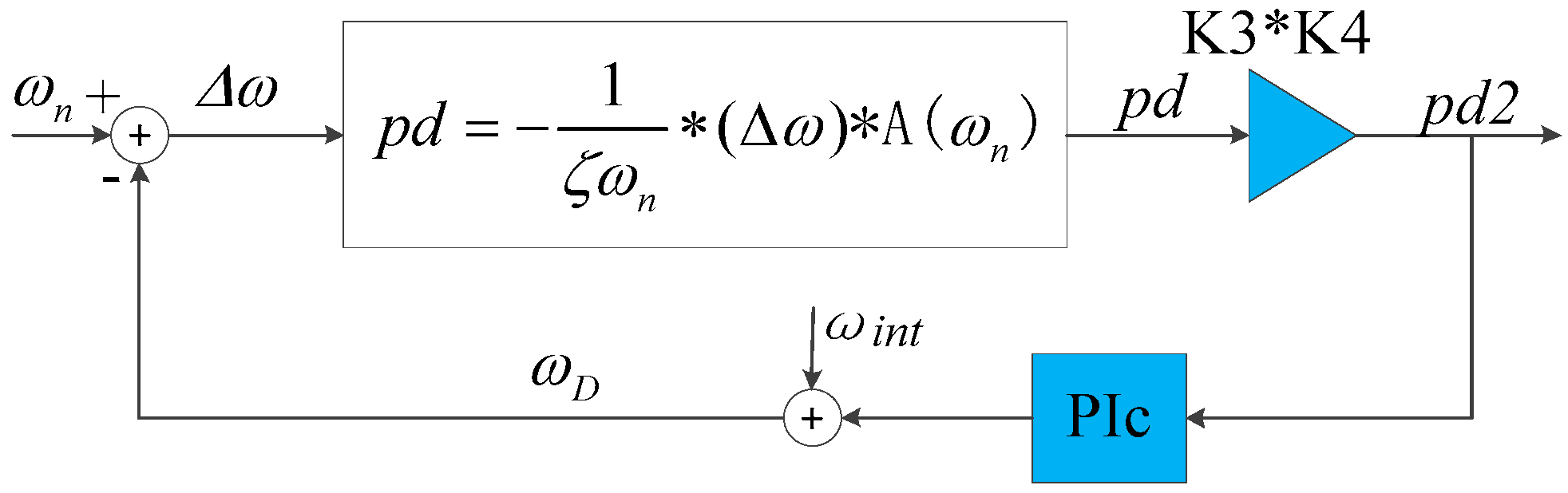
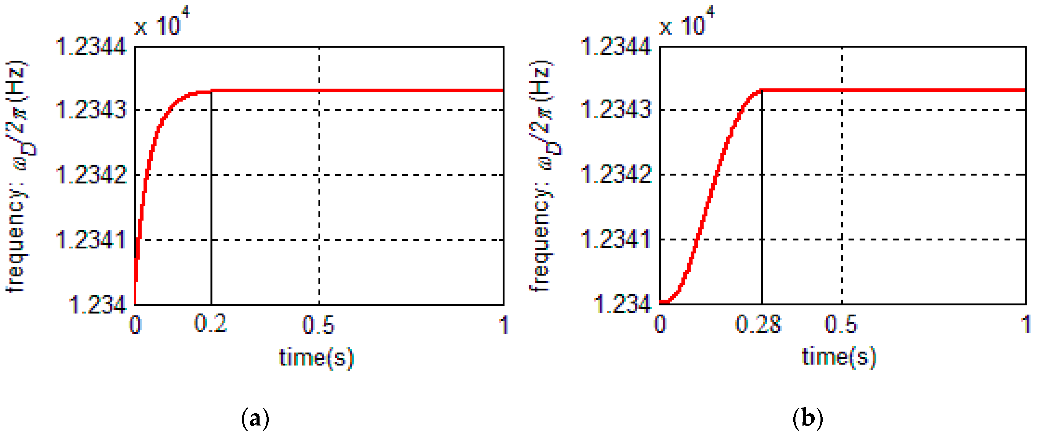
3.2. PLL Model Linearizing and Closed-Loop Design
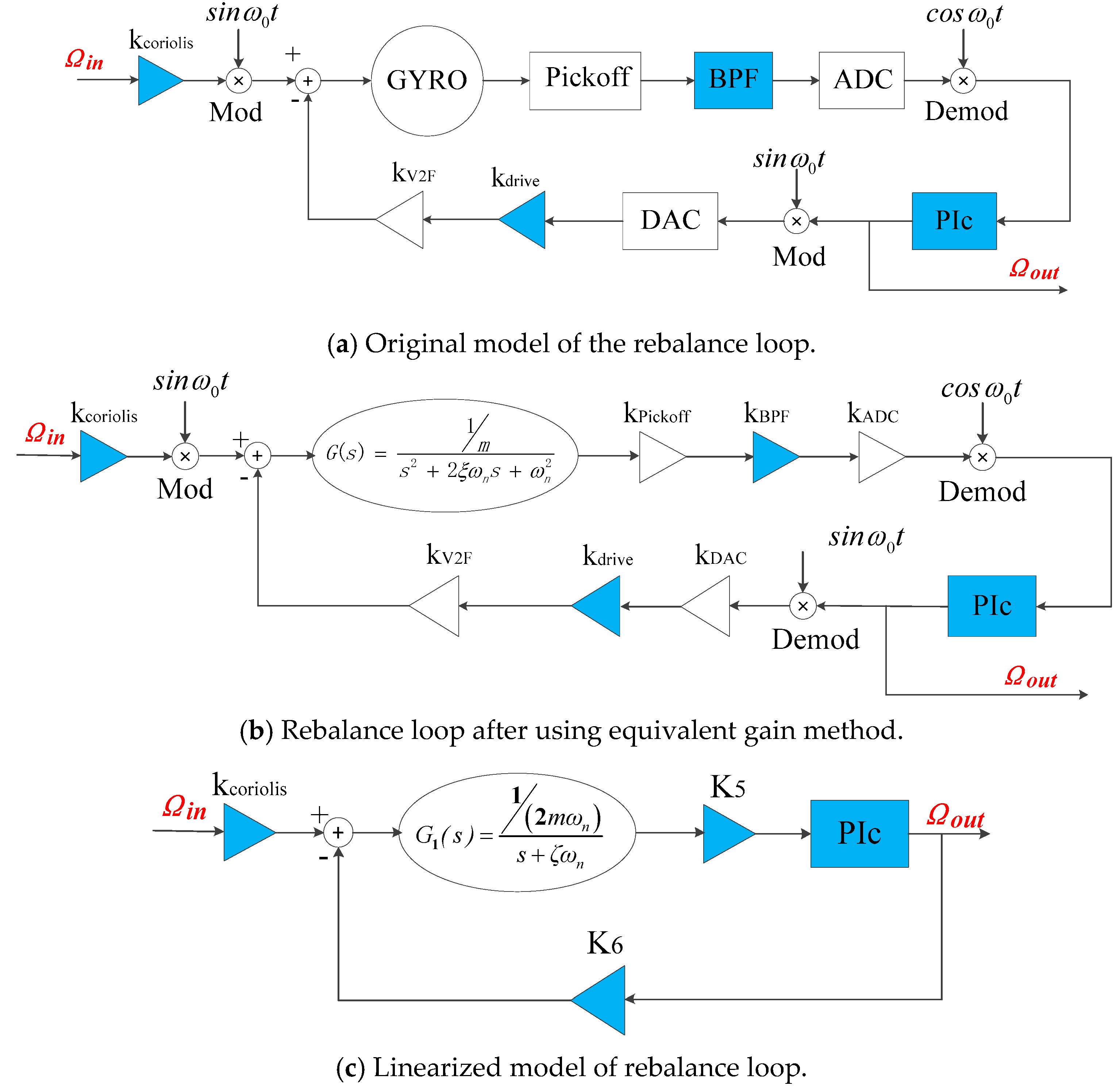
4. Model Linearizing and Performance Analysis of Rebalance Loop
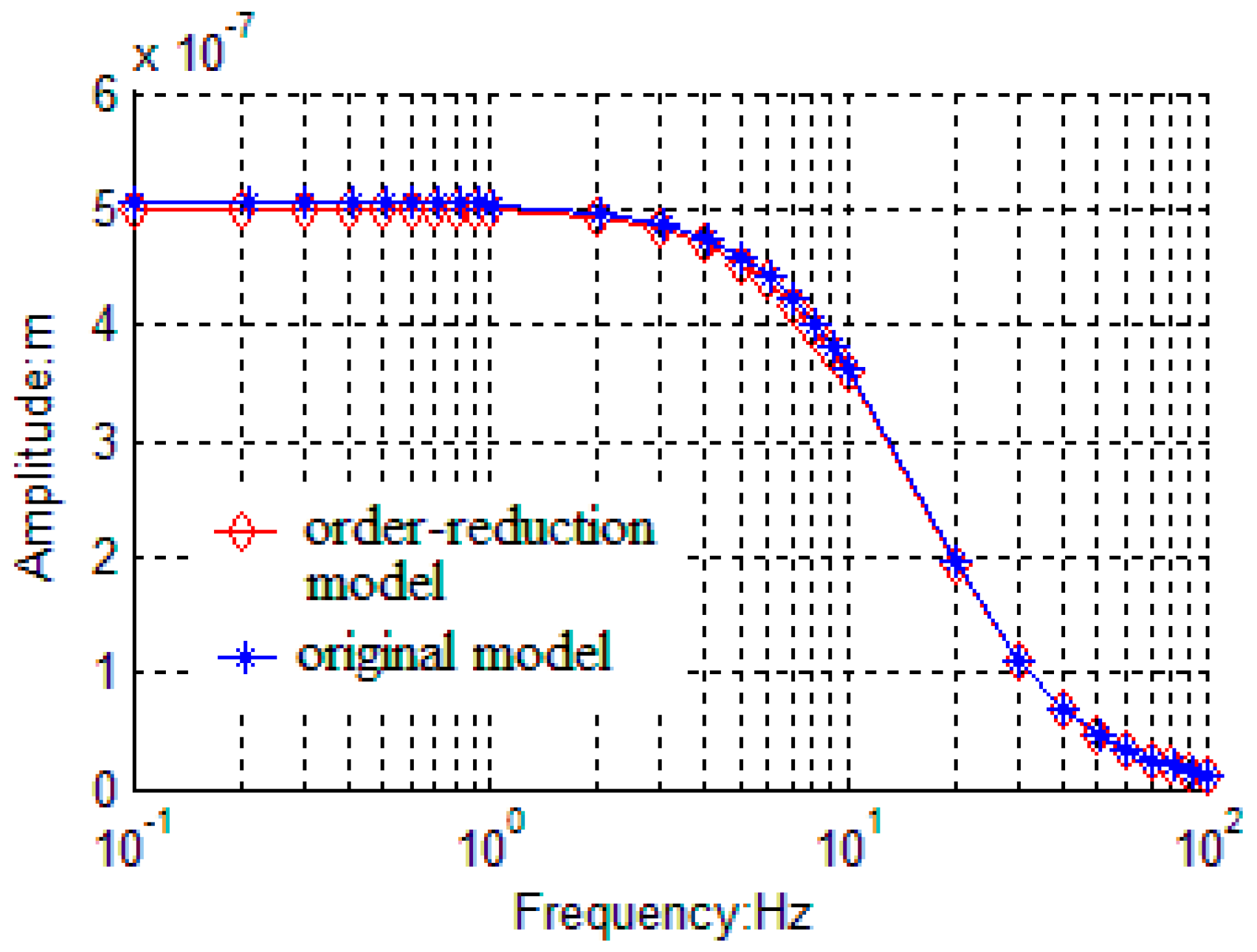
4.1. Model Order-Reduction and Closed-Loop Design of Rebalance Loop
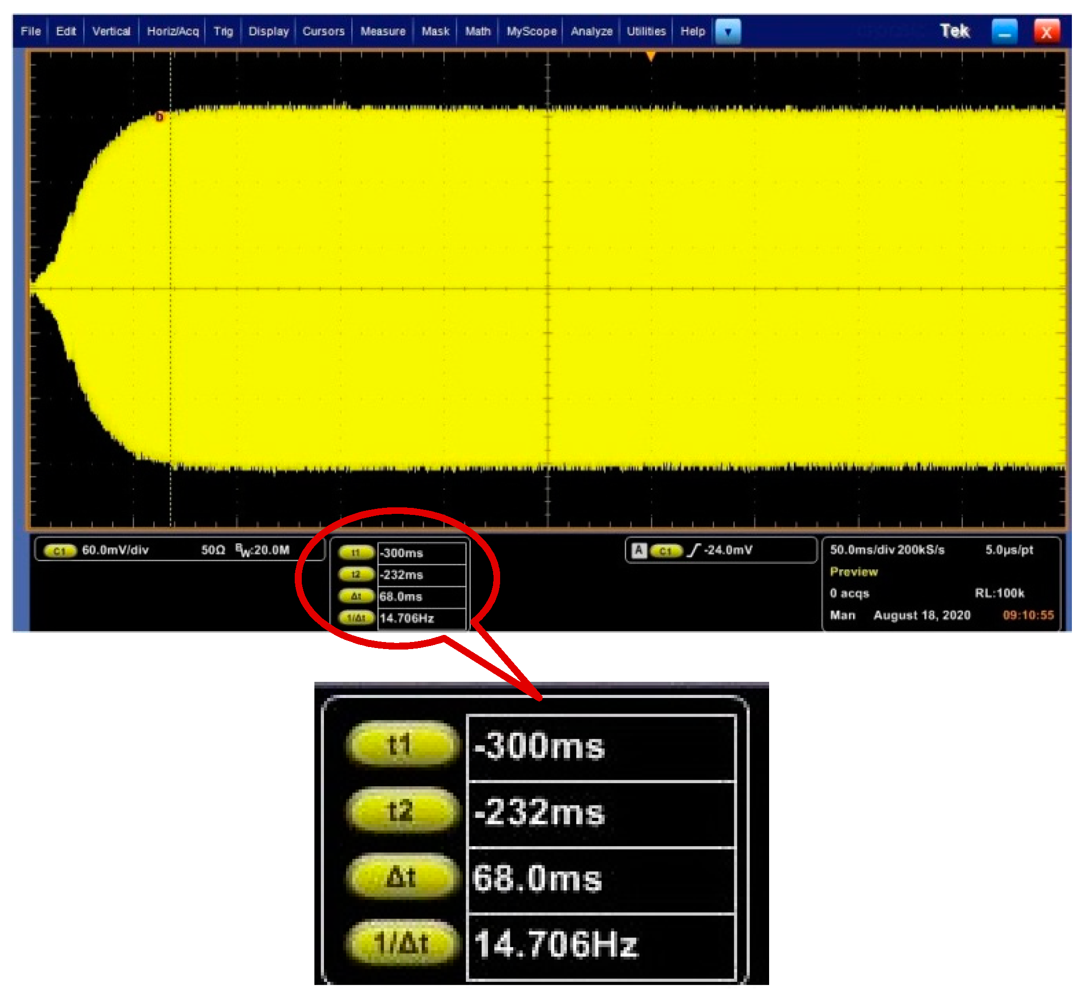
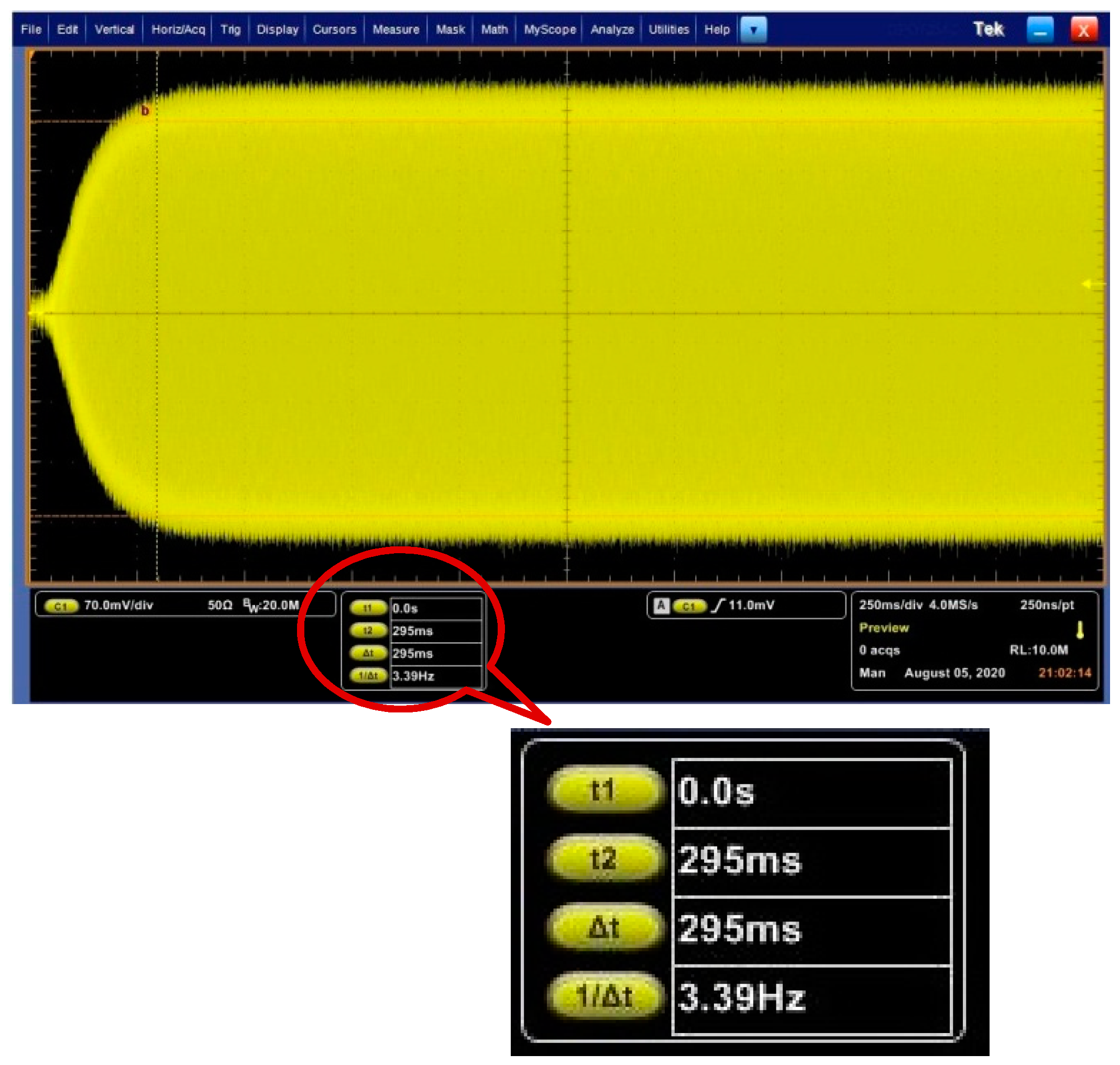
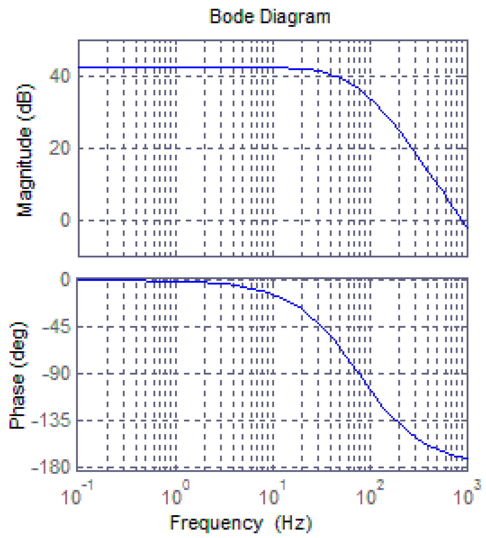
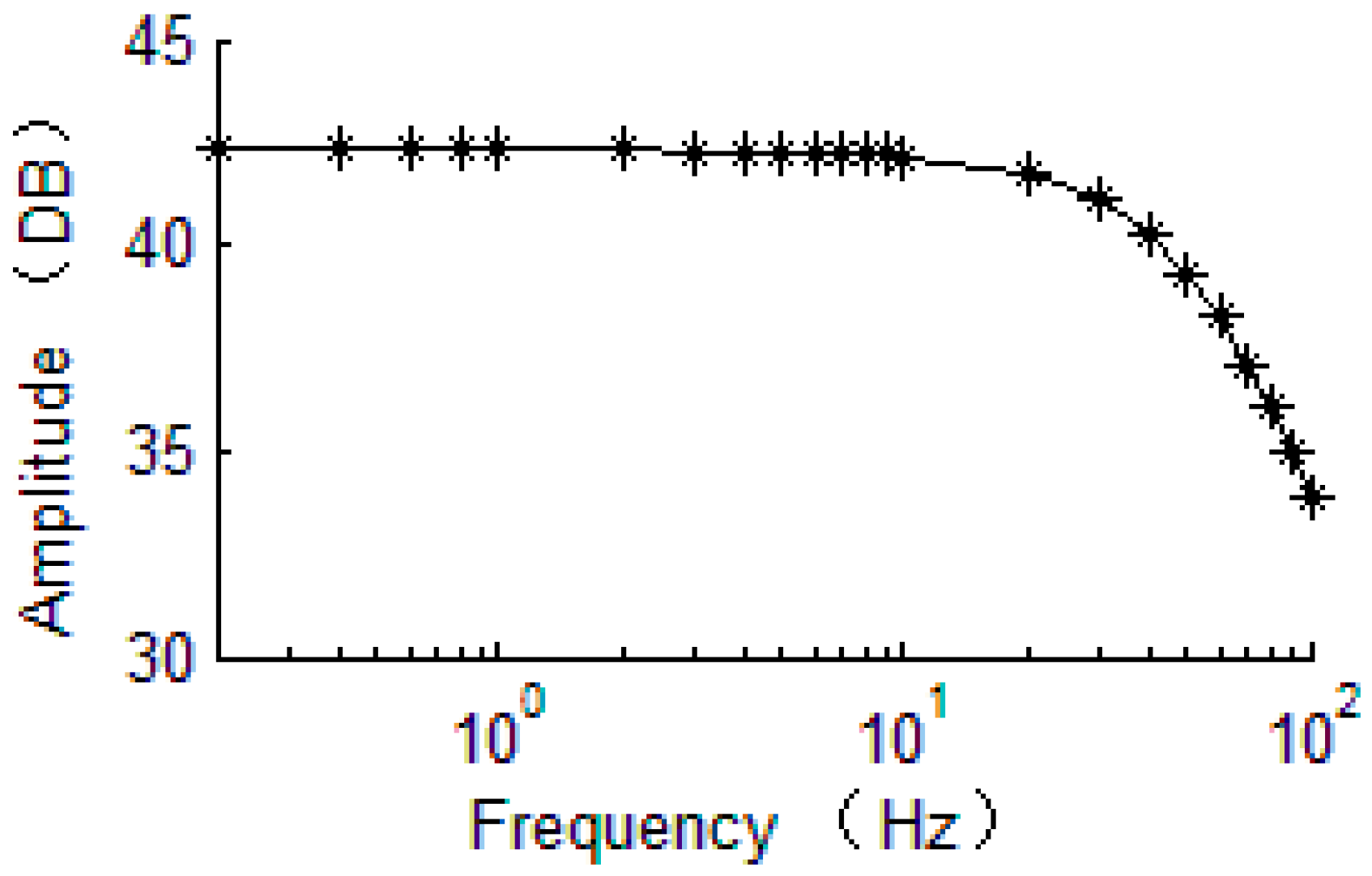
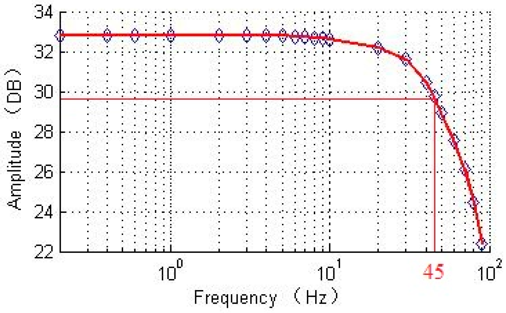
4.2. Bandwidth Analysis
5. Discussion
Author Contributions
Funding
Acknowledgments
Conflicts of Interest
References
- Challoner, A.D.; Ge, H.H.; Liu, J.Y. Boeing disc resonator gyroscope. In Proceedings of the 2014 IEEE/ION Position, Location and Navigation Symposium—PLANS 2014, Monterey, CA, USA, 5–8 May 2014; pp. 504–514. [Google Scholar]
- Shcheglov, K.V.; Dorian Challoner, A. Isolated Planar Gyroscope with Internal Radial Sensing and Actuation. U.S. Patent No. 7040163, 9 May 2006. [Google Scholar]
- Kubena, R.L.; David, T.C. Disc Resonator Gyroscopes. U.S. Patent No. 7581443, 1 September 2009. [Google Scholar]
- Dorian Challoner, A.; David, W. Disc Resonator Integral Inertial Measurement Unit. U.S. Patent No. 7836765, 23 November 2010. [Google Scholar]
- Senkal, D.; Askari, S.; Ahamed, M.J.; Ng, E.J.; Hong, V.; Yang, Y.; Ahn, C.H.; Kenny, T.W.; Shkel, A.M. 100K Q-factor toroidal ring gyroscope implemented in wafer-level epitaxial silicon encapsulation process. In Proceedings of the 2014 IEEE 27th International Conference on Micro Electro Mechanical Systems (MEMS), San Francisco, CA, USA, 26–30 January 2014. [Google Scholar]
- Gerrard, D.D.; Ahn, C.H.; Flader, I.B.; Chen, Y.; Ng, E.J.; Yang, Y.; Kenny, T.W. Q-factor optimization in disk resonator gyroscopes via geometric parameterization. In Proceedings of the 2016 IEEE 29th International Conference on Micro Electro Mechanical Systems (MEMS), Shanghai, China, 24–28 January 2016. [Google Scholar]
- Zhou, X.; Xiao, D.; Hou, Z.; Li, Q.; Wu, Y.; Yu, D.; Li, W.; Wu, X. Thermoelastic quality-factor enhanced disk resonator gyroscope. In Proceedings of the 2017 IEEE 30th International Conference on Micro Electro Mechanical Systems (MEMS), Las Vegas, NV, USA, 22–26 January 2017. [Google Scholar]
- Zhou, X.; Xiao, D.; Li, Q.; Hou, Z.; He, K.; Chen, Z.; Wu, Y.; Wu, X. Decaying Time Constant Enhanced MEMS Disk Resonator for High Precision Gyroscopic Application. IEEE/ASME Trans. Mech. 2016, 23, 452–458. [Google Scholar] [CrossRef]
- Ahn, C.H.; Ng, E.J.; Hong, V.A.; Yang, Y.; Lee, B.J.; Flader, I.; Kenny, T.W. Mode-Matching of Wineglass Mode Disk Resonator Gyroscope in (100) Single Crystal Silicon. J. Mciroelectromech. Syst. 2015, 24, 343–350. [Google Scholar] [CrossRef]
- Lader, I.B.; Ahn, C.H.; Ng, E.J.; Yang, Y.; Hong, V.A.; Kenny, T.W. Stochastic method for disk resonating gyroscope mode matching and quadrature nulling. In Proceedings of the 2016 IEEE 29th International Conference on Micro Electro Mechanical Systems (MEMS), Shanghai, China, 24–28 January 2016. [Google Scholar]
- Xiao, D.; Yu, D.; Zhou, X.; Hou, Z.; He, H.; Wu, X. Frequency Tuning of a Disk Resonator Gyroscope via Stiffness Perturbation. IEEE Sens. J. 2017, 17, 4725–4734. [Google Scholar] [CrossRef]
- Xiao, D.; Zhou, X.; Li, Q.; Hou, Z.; Xi, X.; Wu, Y.; Wu, X. Design of a Disk Resonator Gyroscope With High Mechanical Sensitivity by Optimizing the Ring Thickness Distribution. J. Microelectromech. Syst. 2016, 25, 606–616. [Google Scholar] [CrossRef]
- Zhou, X.; Xiao, D.; Hou, Z.; Li, Q.; Wu, Y.; Wu, X. Influences of the Structure Parameters on Sensitivity and Brownian Noise of the Disk Resonator Gyroscope. J. Microelectromech. Syst. 2017, 26, 519–527. [Google Scholar] [CrossRef]
- HyuckAhn, C.; Shin, D.D.; Hong, V.A.; Yang, Y.; Ng, E.J.; Chen, Y.; Flader, I.B.; Kenny, T.W. Encapsulated disk resonator gyroscope with differential internal electrodes. In Proceedings of the 2016 IEEE 29th International Conference on Micro Electro Mechanical Systems (MEMS), Shanghai, China, 24–28 January 2016. [Google Scholar]
- Shen, Q.; Chang, H.; Wu, Y.; Xie, J. Turn-on bias behavior prediction for micromachined Coriolis vibratory gyroscopes. Measuremernt 2019, 131, 380–393. [Google Scholar] [CrossRef]
- Chorsi, H.T.; Chorsi, M.T.; Gedney, S.D. A Conceptual Study of Microelectromechanical Disk Resonators. IEEE J. Multiscale Multiphysics Comput. Tech. 2017, 2, 29–37. [Google Scholar] [CrossRef]
- Chorsi, M.T.; Chorsi, H.T. Systematic analysis of carbon-based microdisk resonators. FlatChem 2020, 20, 100159. [Google Scholar] [CrossRef]
- Chorsi, M.T.; Chorsi, H.T. Modeling and analysis of MEMS disk resonators. Microsyst. Technol. 2018, 24, 2517–2528. [Google Scholar] [CrossRef]
- Chorsi, M.T.; Chorsi, H.T.; Gedney, S.D. Radial-contour mode microring resonators: Nonlinear dynamics. Int. J. Mech. Sci. 2017, 130, 258–266. [Google Scholar] [CrossRef]
- Ahn, C.; Hong, V.; Park, W.; Yang, Y.; Chen, Y.; Ng, E.; Huynh, J.; Challoner, A.; Goodson, K.; Kenny, T. On-chip ovenization of encapsulated Disk Resonator Gyroscope (DRG). In Proceedings of the 2015 Transducers—2015 18th International Conference on Solid-State Sensors, Actuators and Microsystems (TRANSDUCERS), Anchorage, AK, USA, 21–25 June 2015. [Google Scholar]
- Dion, F.; Martel, S.; DeNatale, J. 200mm High Performance Inertial Sensor Manufacturing Process. In Proceedings of the 2018 IEEE International Symposium on Inertial Sensors and Systems (INERTIAL), Moltrasio, Italy, 26–29 March 2018. [Google Scholar]
- Sung, W.-T.; Sung, S.; Lee, J.G.; Kang, T. Design and performance test of a MEMS vibratory gyroscope with a novel AGC force rebalance control. J. Micromech. Microeng. 2007, 17, 1939–1948. [Google Scholar] [CrossRef]
- Cui, J.; Chi, X.Z.; Ding, H.T.; Lin, L.T.; Yang, Z.C.; Yan, G.Z. Transient response and stability of the AGC-PI closed-loop controlled MEMS vibratory gyroscopes. J. Micromech. Microeng. 2009, 19, 1–17. [Google Scholar] [CrossRef]
- Kraft, M.; Wilcock, R.; Almutairi, B. Innovative control systems for MEMS inertial sensors. In Proceedings of the 2012 IEEE International Frequency Control Symposium Proceedings, Baltimore, MD, USA, 21–24 May 2012. [Google Scholar]
- Chen, F.; Yuan, W.; Chang, H.; Yuan, G.; Xie, J.; Kraft, M. Design and Implementation of an Optimized Double Closed-Loop Control System for MEMS Vibratory Gyroscope. IEEE Sens. J. 2013, 14, 184–196. [Google Scholar] [CrossRef]
- Keymeulen, D.; Peay, C.; Foor, D.; Trung, T.; Bakhshi, A.; Withington, P.; Yee, K.; Terrile, R. Control of MEMS Disc Resonance Gyroscope (DRG) using a FPGA Platform. In Proceedings of the 2008 IEEE Aerospace Conference, Big Sky, MT, USA, 1–8 March 2008. [Google Scholar]
- Polunin, P.M.; Shaw, S.W. Self-induced parametric amplification in ring resonating gyroscopes. Int. J. Nonlin. Mech. 2017, 94, 300–308. [Google Scholar]
- Wang, H.; Ye, Z.; Zhang, Q.; Quan, H. System modeling, simulation and parameter analysis of MEMS vibrating ring gyroscope. Navig. Control 2017, 16, 25–32. [Google Scholar]
- Sharma, M.; Kannan, A.; Cretu, E. Noise-based optimization and noise analysis for resonant MEMS structures. In Proceedings of the 2008 Symposium on Design, Test, Integration and Packaging of MEMS/MOEMS, Nice, France, 9–11 April 2008. [Google Scholar]
- Putty, M. A micromachined vibrating ring gyroscope. Ph.D. Thesis, University of Michigan, Ann Arbor, MI, USA, 1995. [Google Scholar]
- Zhang, A. Automatic Control Theory, 1st ed.; Tsinghua University Press: Beijing, China, 2006; pp. 154–196. [Google Scholar]


| Parameter | Value |
|---|---|
| Effective mass/m | 1.67 × 10⁻⁶ kg |
| Q factor/Q | 13,000 |
| Resonant frequency/f0 | 12,343.3 Hz |
| Angular gain/Ag | 0.393 |
| Sense capacitance/C0 | 7.6 pF |
| Drive capacitance/Cdrive | 3.4 pF |
| Electrodes’ spacing/x0 | 5 μm |
| Primary amplitude/Ax | 0.5 μm |
| Feedback capacitance of CV/Cf | 10 pF |
| DC bias voltage/Vbias | 10 V |
| Key Parts of ASIC | Specification | Value |
|---|---|---|
| Pickoff circuit/CV | To pickoff the displacement of resonator | |
| DAC/ADC | 20-bit sigma-delta ADCs and 16-bit sigma-delta DACs | , |
| Band-pass filter | The central frequency is configurable | |
| Drive circuit | To provide the drive capability for DRG | Gain is configurable |
| Electrostatic feedback force | - | |
| Gain of Coriolis force | - | |
| PI controller | Implemented in an embedded MCU and is configurable | , configurable |
Publisher’s Note: MDPI stays neutral with regard to jurisdictional claims in published maps and institutional affiliations. |
© 2020 by the authors. Licensee MDPI, Basel, Switzerland. This article is an open access article distributed under the terms and conditions of the Creative Commons Attribution (CC BY) license (http://creativecommons.org/licenses/by/4.0/).
Share and Cite
Wang, H.; Wang, X.; Xie, J. First-Order Linear Mechatronics Model for Closed-Loop MEMS Disk Resonator Gyroscope. Sensors 2020, 20, 6455. https://doi.org/10.3390/s20226455
Wang H, Wang X, Xie J. First-Order Linear Mechatronics Model for Closed-Loop MEMS Disk Resonator Gyroscope. Sensors. 2020; 20(22):6455. https://doi.org/10.3390/s20226455
Chicago/Turabian StyleWang, Hao, Xiupu Wang, and Jianbing Xie. 2020. "First-Order Linear Mechatronics Model for Closed-Loop MEMS Disk Resonator Gyroscope" Sensors 20, no. 22: 6455. https://doi.org/10.3390/s20226455
APA StyleWang, H., Wang, X., & Xie, J. (2020). First-Order Linear Mechatronics Model for Closed-Loop MEMS Disk Resonator Gyroscope. Sensors, 20(22), 6455. https://doi.org/10.3390/s20226455