Establishment of a New Quantitative Evaluation Model of the Targets’ Geometry Distribution for Terrestrial Laser Scanning

Abstract

The precision of target-based registration is related to the geometry distribution of targets, while the current method of setting the targets mainly depends on experience, and the impact is only evaluated qualitatively by the findings from empirical experiments and through simulations. In this paper, we propose a new quantitative evaluation model, which is comprised of the rotation dilution of precision ($rDOP$, assessing the impact of targets’ geometry distribution on the rotation parameters) and the translation dilution of precision ($tDOP$, assessing the impact of targets’ geometry distribution on the translation parameters). Here, the definitions and derivation of relevant formulas of the $rDOP$ and $tDOP$ are given, the experience conclusions are theoretically proven by the model of $rDOP$ and $tDOP$, and an accurate method for determining the optimal placement location of targets and the scanner is proposed by calculating the minimum value of $rDOP$ and $tDOP$. Furthermore, we can refer to the model ($rDOP$ and $tDOP$) as a unified model of the geometric distribution evaluation model, which includes the $DOP$ model in GPS.

1. Introduction

Terrestrial laser scanning (TLS) can provide a three-dimensional (3D) spatial point cloud dataset of the objects’ surfaces. The spatial resolution of the data is much higher than that of conventional surveying methods [1]. Due to occluded surfaces and limitations in the view of a scanner, we usually need to make several scans from different setups of the scanner in order to survey a quite large and complex object [2,3]. These point clouds (scans) must first be registered to a chosen coordinate system before a coherent parametric description of the object can be formed [4]. Target-based registration with two scans is one of the most common registration approaches and is often performed using a 3D rigid body transformation algorithm [5,6].

Although target-based registration technology is relatively mature [7], studies of the target-based registration precision are still required, such as those on measurement improvement [8,9], the uncertainty of the target center estimation [10], the error propagation for two scans and multiple scans [3,4,11], the directly geo-referenced TLS data precision [3,12], the relationship between the registration precision and the rotation and translation matrices [13], the relationship between the registration precision and the targets’ geometry distribution (TGD) [2], etc. For the relationship between the registration precision and TGD, some researchers have found that an increase in the number of targets can improve the registration precision, and think that the targets will be distributed evenly and will not lie on the same line or be close to such a configuration [2,14,15,16,17,18,19,20]. Fan et al. [12] and Liu et al. [17] used a simulation method to demonstrate that the registration error is inversely proportional to the number of targets and the sum of distances between targets and the barycenter of all targets. Bornaz et al. [21] proved that the registration precision of two scans depends on the overlap ratio adopted (namely the target distribution range of the overlap area), and found that the minimum overlap ratio of 30% is required for assuring a final precision comparable to the range precision of the used instruments. However, all of the above studies have only evaluated the impact of TGD on the registration precision qualitatively through empirical experiments and simulations, while there has been no research conducted on the theoretical evaluation model for it. As a result, we can never know the best location of the scanner and the best TGD. How can we quantitatively evaluate the impact of TGD and describe the relationship between TGD and registration precision? These issues are the focus of this research.

In this study, we first used the theorem of error propagation to constitute a new theoretical evaluation model of the TGD, that is, the rotation dilution of precision ($rDOP$) and the translation dilution of precision ($tDOP$); we then theoretically analyzed the model’s existence conditions, the relationship between the model and the number of targets, and the model’s bounds; and finally, we verified the evaluation model of the TGD by conducting experiments.

2. Methods

There are two kinds of situations in practical applications, which are “we need to determine the optimal setting position of scanner where TGD is known” and “we need to determine the optimal TGD where the position of scanner is known”. The unit of the rotation parameters is different from the unit of translation parameters, and the calculation results of translation and rotation will interact with each other when the transformation parameters are dependent on calculation models. For these reasons, we will first introduce the common registration model of two scans. We will then present the calculation of rotation parameters using the Rodrigues matrix [3,6]. Thirdly, we will propose a new calculation method of the translation parameter (similar to spatial distance resection in GPS [22]), which can ensure that the parameters of translation and rotation are computed independently. Fourthly, we will propose a new quantitative evaluation model of TGD, namely $rDOP$ (which can be used to help determine the optimal TGD) and $tDOP$ (which can be used to help determine the optimal setting position of scanner). Finally, we will derive an equal weight model of TGD and propose a set of model application schemes.

2.1. Registration Model of Two Scans

In the context of TLS, registration is the transformation of multiple point clouds (scans) into the coordinate system of a chosen scan [2]. The rigid body transformation operation of registration is expressed in Equation (1), in which the point clouds in Scan i + 1 are transformed into Scan i using the three translation parameters $t_x$, $t_y$, and $t_z$ and the three rotation parameters $r_a$, $r_b$, and $r_c$ [3,23].

$$p_j^i=\left[\begin{array}{c}{x}_j^i\\ y_j^i\\ z_j^i\end{array}\right]=R\left[\begin{array}{c}{x}_j^{i+1}\\ y_j^{i+1}\\ z_j^{i+1}\end{array}\right]+T=R{p}_j^{i+1}+T,$$

(1)

where $p_j^i$ and $p_j^{i+1}$ represent the same target in Scan i and Scan i + 1, respectively, whose observation values of coordinates are $(x_j^i,y_j^i,z_j^i)$ and $(x_j^{i+1},y_j^{i+1},z_j^{i+1})$; $R$ is the standard $3\times 3$ rotation matrix; $T$ is the $3\times 1$ translation vector; and

$$R=\frac{1}{1+r_a^2+r_b^2+r_c^2}\left[\begin{array}{ccc}1+r_a^2-r_b^2-r_c^2& 2(r_c+r_a{r}_b)& 2(r_a{r}_c-r_b)\\ 2(r_a{r}_b-r_c)& 1-r_a^2+r_b^2-r_c^2& 2(r_a+r_b{r}_c)\\ 2(r_b+r_a{r}_c)& 2(r_b{r}_c-r_a)& 1-r_a^2-r_b^2+r_c^2\end{array}\right],T=\left[\begin{array}{c}{t}_x\\ t_y\\ t_z\end{array}\right].$$

(2)

For uniquely determining the above transformation parameters between Scan i and Scan Scan i + 1, we usually need to use three or more targets with known 3D coordinates [2,21], and these targets are placed in the overlap locations between the two point-clouds.

In this study, we assumed that the number of targets $k$ is greater than 3 ($k\ge 3$) and the coordinate of any point in Scan i (on a chosen coordinate system) is known, and we employed scanning to obtain the new point cloud in Scan Scan i + 1, which was transformed into Scan i.

2.2. Calculation of Rotation Parameters

If $p_{jc}^i=p_j^i-\frac{1}{k}{\displaystyle \sum _{j_m=1}^k{p}_{j_m}^i}$ and $p_{jc}^{i+1}=p_j^{i+1}-\frac{1}{k}{\displaystyle \sum _{j_m=1}^k{p}_{j_m}^{i+1}}$, with Equation (1), we can get

$$p_{jc}^i=\left[\begin{array}{c}{x}_{jc}^i\\ y_{jc}^i\\ z_{jc}^i\end{array}\right]=R\left[\begin{array}{c}{x}_{jc}^{i+1}\\ y_{jc}^{i+1}\\ z_{jc}^{i+1}\end{array}\right]=R{p}_{jc}^{i+1}.$$

(3)

From the Rodrigues matrix [21,23], with Equations (2) and (3), we can get

$$(I_3+S)\left[\begin{array}{c}{x}_{jc}^i\\ y_{jc}^i\\ z_{jc}^i\end{array}\right]=(I_3-S)\left[\begin{array}{c}{x}_{jc}^{i+1}\\ y_{jc}^{i+1}\\ z_{jc}^{i+1}\end{array}\right],$$

(4)

where $S=\left[\begin{array}{ccc}0& -r_c& r_b\\ r_c& 0& -r_a\\ -r_b& r_a& 0\end{array}\right]$ and $R={(I_3+S)}^{-1}(I_3-S)$.

With Equation (4), we can get

$${\alpha }_j\left[\begin{array}{c}{r}_a\\ r_b\\ r_c\end{array}\right]=p_{jc}^i-p_{jc}^{i+1},j=1,2,\cdots ,k,$$

(5)

where $S=\left[\begin{array}{ccc}0& -r_c& r_b\\ r_c& 0& -r_a\\ -r_b& r_a& 0\end{array}\right]$ and $R={(I_3+S)}^{-1}(I_3-S)$.

$${\alpha }_j=\left[\begin{array}{ccc}0& -{\tau }_{z,j}& {\tau }_{y,j}\\ {\tau }_{z,j}& 0& -{\tau }_{x,j}\\ -{\tau }_{y,j}& {\tau }_{x,j}& 0\end{array}\right],\left[\begin{array}{c}{\tau }_{x,j}\\ {\tau }_{y,j}\\ {\tau }_{z,j}\end{array}\right]=\left[\begin{array}{c}{x}_{jc}^i+x_{jc}^{i+1}\\ y_{jc}^i+y_{jc}^{i+1}\\ z_{jc}^i+z_{jc}^{i+1}\end{array}\right]=p_{jc}^i+p_{jc}^{i+1}=(I_3+R)p_{jc}^i.$$

(6)

If the estimated values of $r_a$, $r_b$, and $r_c$ are ${\widehat{r}}_a$, ${\widehat{r}}_b$, and ${\widehat{r}}_c$, respectively, with Equations (5) and (6), the observation equation of rotation parameters can be expressed as

$$A_{r(k)}{\delta }_r=L_{r(k)},$$

(7)

where $A_{r(k)}$, $L_{r(k)}$, and ${\delta }_r$ are $3k\times 3$ matrix, $3k\times 1$ matrix, and $3\times 1$ matrix, respectively, and

$$A_{r(k)}=\left[\begin{array}{c}{\alpha }_1\\ ⋮\\ {\alpha }_k\end{array}\right],L_{r(k)}=\left[\begin{array}{c}{p}_{1c}^i-p_{1c}^{i+1}\\ ⋮\\ p_{kc}^i-p_{kc}^{i+1}\end{array}\right],{\delta }_r=\left[\begin{array}{c}{\widehat{r}}_a\\ {\widehat{r}}_b\\ {\widehat{r}}_c\end{array}\right].$$

(8)

Assuming the weight matrix of $L_{r(k)}$ is $P_{r(k)}$, by using the principle of indirect adjustment [24] and $V^{T}PV=\min$, we can obtain the estimated ${\delta }_r$ for rotation parameters as

$${\delta }_r={(A_{r(k)}^T{P}_{r(k)}{A}_{r(k)})}^{-1}{A}_{r(k)}^T{P}_{r(k)}{L}_{r(k)}.$$

(9)

2.3. Calculation of Translation Parameters

As the position of scanner i + 1 in Scan i + 1 is $(0,0,0)$, with Equation (1), we can find that the position of scanner i + 1 in Scan i is equal to the value of $T$, namely, the process of determining translation parameters is equivalent to solving the position of scanner i + 1 in Scan i. If the targets are regarded as GPS satellites, scanner i + 1 is regarded as a GPS receiver, and the calculation method of translation parameters is equivalent to solving the position of the GPS receiver by GPS satellites, namely, spatial distance resection in GPS [22], which will not be affected by the estimated precision of rotation parameters.

If the observation value of distance between scanner i + 1 and the jth target in Scan i + 1 is $d_j^{i+1}$, the observation equation of translation parameters can be expressed as

$$\left[\begin{array}{c}{d}_1^{i+1}\\ ⋮\\ d_k^{i+1}\end{array}\right]=\left[\begin{array}{c}\sqrt{{(x_1^i-t_x)}^2+{(y_1^i-t_y)}^2+{(z_1^i-t_z)}^2}\\ ⋮\\ \sqrt{{(x_k^i-t_x)}^2+{(y_k^i-t_y)}^2+{(z_k^i-t_z)}^2}\end{array}\right],$$

(10)

where $d_j^{i+1}=\sqrt{{(x_j^{i+1})}^2+{(y_j^{i+1})}^2+{(z_j^{i+1})}^2}$ and $j=1,2,\cdots ,k$.

If the approximation values of translation parameters and corrections of translation parameters $t_x$, $t_y$, and $t_z$ are $t_{x,0}$, $t_{y,0}$, and $t_{z,0}$ (calculated by the method of Appendix C in [3]) and ${\epsilon }_{t_x}$, ${\epsilon }_{t_y}$, and ${\epsilon }_{t_z}$, then from the linearization theorem [22,24], the linearization form of Equation (10) can be expressed as

$$A_{t(k)}{\delta }_t=L_{t(k)},$$

(11)

where $T=T_0+{\delta }_t$; $A_{t(k)}$, $L_{t(k)}$, and ${\delta }_t$ are $k\times 3$ matrix, $k\times 1$ matrix, $3\times 1$ matrix, respectively; and

$$A_{t(k)}=\left[\begin{array}{c}{\beta }_1\\ ⋮\\ {\beta }_k\end{array}\right]=\left[\begin{array}{ccc}{l}_{x,1}& m_{y,1}& n_{z,1}\\ ⋮& ⋮& ⋮\\ l_{x,k}& m_{y,k}& n_{z,k}\end{array}\right],{\delta }_t=\left[\begin{array}{c}{\epsilon }_{t_x}\\ {\epsilon }_{t_y}\\ {\epsilon }_{t_z}\end{array}\right],L_{t(k)}=\left[\begin{array}{c}{d}_{1,0}^i-d_1^{i+1}\\ ⋮\\ d_{k,0}^i-d_k^{i+1}\end{array}\right],T_0=\left[\begin{array}{c}{t}_{x,0}\\ t_{y,0}\\ t_{z,0}\end{array}\right],$$

(12)

$${\beta }_j=\left[\begin{array}{ccc}{l}_{x,j}& m_{y,j}& n_{z,j}\end{array}\right]=\left[\begin{array}{ccc}\frac{x_j^i-t_{x,0}}{d_{j,0}^i}& \frac{y_j^i-t_{y,0}}{d_{j,0}^i}& \frac{z_j^i-t_{z,0}}{d_{j,0}^i}\end{array}\right],j=1,2,\cdots ,k,$$

(13)

$$d_{j,0}^i=\sqrt{{(x_j^i-t_{x,0})}^2+{(y_j^i-t_{y,0})}^2+{(z_j^i-t_{z,0})}^2}.$$

(14)

Assuming the weight matrix of $L_{t(k)}$ is $P_{t(k)}$, by using the principle of indirect adjustment [24], we can obtain the estimated ${\delta }_t$ for translation parameters as

$${\delta }_t={(A_{t(k)}^T{P}_{t(k)}{A}_{t(k)})}^{-1}{A}_{t(k)}^T{P}_{t(k)}{L}_{t(k)}.$$

(15)

2.4. Quantitative Evaluation Model of TGD

With Equations (9) and (15), based on the theorem of error propagation [24], the covariance $D_{{\delta }_r{\delta }_r}$ and $D_{{\delta }_t{\delta }_t}$ of the rotation parameters ${\delta }_r$ and the translation parameter corrections ${\delta }_t$ can be obtained as

$$\{\begin{array}{l}{D}_{{\delta }_r{\delta }_r}={(A_{r(k)}^T{P}_{r(k)}{A}_{r(k)})}^{-1}{\sigma }_0^2\\ D_{{\delta }_t{\delta }_t}={(A_{t(k)}^T{P}_{t(k)}{A}_{t(k)})}^{-1}{\sigma }_0^2\end{array},$$

(16)

where $D_{{\delta }_r{\delta }_r}$ and $D_{{\delta }_t{\delta }_t}$ are $3\times 3$ matrices, and ${\sigma }_0$ is the unit weight variance, usually determined in the initial processing before registration.

As the trace of a real-symmetric matrix is equal to the trace of its corresponding diagonal matrix and the parameters’ variance-covariance matrix is a real-symmetric matrix, we usually use the trace of the parameters’ variance-covariance matrix in the precision evaluation of parameters, such as point precision evaluation. For this reason, we assume that the variances of rotation parameters ${\widehat{r}}_a$, ${\widehat{r}}_b$, and ${\widehat{r}}_c$ and the translation parameters’ corrections ${\epsilon }_{t_x}$, ${\epsilon }_{t_y}$, and ${\epsilon }_{t_z}$ are ${\sigma }_a$, ${\sigma }_b$, ${\sigma }_c$, ${\sigma }_{t_x}$, ${\sigma }_{t_y}$, and ${\sigma }_{t_z}$, respectively. With Equation (16), the registration precision (namely, the variances of parameters ${\delta }_r$ and ${\delta }_t$) can be obtained as

$$\sqrt{{\sigma }_a^2+{\sigma }_b^2+{\sigma }_c^2}=tr(\sqrt{D_{{\delta }_r{\delta }_r}})=tr(\sqrt{{(A_{r(k)}^T{P}_{r(k)}{A}_{r(k)})}^{-1}}){\sigma }_0,$$

(17)

$$\sqrt{{\sigma }_{t_x}^2+{\sigma }_{t_y}^2+{\sigma }_{t_z}^2}=tr(\sqrt{D_{{\delta }_t{\delta }_t}})=tr(\sqrt{{(A_{t(k)}^T{P}_{t(k)}{A}_{t(k)})}^{-1}}){\sigma }_0,$$

(18)

where tr(.) is the trace of the matrix.

In GPS positioning, the impact of the satellites’ geometry distribution on the positioning quality is evaluated by the dilution of precision ($DOP$) values [25,26,27]. Similarly, we can also build a quantitative evaluation model of the impact of TGD on the registration precision, that is, the rotation dilution of precision ($rDOP$) and the translation dilution of precision ($tDOP$), namely

$$rDOP=\sqrt{tr(G_k^{-1})},$$

(19)

$$tDOP=\sqrt{tr(H_k^{-1})},$$

(20)

where $G_k=A_{r(k)}^T{P}_{r(k)}{A}_{r(k)}$ and $H_k=A_{t(k)}^T{P}_{t(k)}{A}_{t(k)}$.

With Equations (17)–(20), we can find that the registration precision of rotation parameters and translation parameters are

$$\sqrt{{\sigma }_a^2+{\sigma }_b^2+{\sigma }_c^2}=rDOP\cdot {\sigma }_0,$$

(21)

$$\sqrt{{\sigma }_{t_x}^2+{\sigma }_{t_y}^2+{\sigma }_{t_z}^2}=tDOP\cdot {\sigma }_0.$$

(22)

From the above evaluation model of TGD, we can find that

• The values of $rDOP$ and $tDOP$ represent the amplification of the unit weight variance, which means the lower the values of $rDOP$ and $tDOP$, the higher the solution precisions of the rotation parameters and the translation parameters;
• The values of $rDOP$ calculated by Equation (19) are related to the coefficient matrix $A_{r(k)}$ and the weight matrix $P_{r(k)}$ of $L_{r(k)}$, among which $A_{r(k)}$ is related to TGD (the coordinates of targets $p_{jc}^i$) and the rotation matrix $R$. Namely, when $R$ is fixed, the better the quality of TGD, the lower the values of $rDOP$;
• The values of $tDOP$ calculated by Equation (20) are related to the coefficient matrix $A_{t(k)}$; and the weight matrix $P_{t(k)}$ of $L_{t(k)}$, among which $A_{t(k)}$ is related to TGD (the coordinates of targets $p_j^i$) and the position of scanner i + 1 in Scan i. Namely, the better the quality of TGD and the position of scanner i + 1, the lower the values of $tDOP$;
• The calculation formula of $tDOP$ is identical to the calculation formula of $DOP$ in GPS, so the $tDOP$ can be used to evaluate the quality of the received GPS satellites’ distribution. Namely, the $rDOP$ and $tDOP$ model is a unified evaluation model of the targets’ and GNSS satellites’ geometric distribution.

2.5. Equationuationual Weight Model of $rDOP$ and $tDOP$

In constituting the $DOP$ model for evaluating the impact of the selected GNSS satellite geometry [25,26,27], we usually assume that the weight matrix is an identity matrix. Additionally, in all the empirical experiments and simulations of the TGD impact on the registration precision [2,12,14,15,16,17,18,19,20], we assume that the weight matrix is an identity matrix. For these reasons and for convenience of the following analysis on the nature of the $rDOP$ and $tDOP$ model, we assume that $P_{r(k)}$ and $P_{t(k)}$ are equal to identity matrix $I$, and use the equal weight least squares method to compute the registration parameters in Equations (9) and (15). With Equations (6)–(8) and Equations (12)–(14), we then get

$$G_k=A_{r(k)}^T{A}_{r(k)}={\displaystyle \sum _{j=1}^k\left[\begin{array}{ccc}{\tau }_j^2-{\tau }_{x,j}^2& -{\tau }_{x,j}{\tau }_{y,j}& -{\tau }_{x,j}{\tau }_{z,j}\\ -{\tau }_{x,j}{\tau }_{y,j}& {\tau }_j^2-{\tau }_{y,j}^2& -{\tau }_{y,j}{\tau }_{z,j}\\ -{\tau }_{x,j}{\tau }_{z,j}& -{\tau }_{y,j}{\tau }_{z,j}& {\tau }_j^2-{\tau }_{z,j}^2\end{array}\right]},$$

(23)

$$H_k=A_{t(k)}^T{A}_{t(k)}={\displaystyle \sum _{j=1}^k\left[\begin{array}{ccc}{l}_{x,j}^2& -l_{x,j}{m}_{y,j}& -l_{x,j}{n}_{z,j}\\ -l_{x,j}{m}_{y,j}& l_{y,j}^2& -m_{y,j}{n}_{z,j}\\ -l_{x,j}{n}_{z,j}& -m_{y,j}{n}_{z,j}& l_{z,j}^2\end{array}\right]},$$

(24)

where ${\tau }_j^2={\tau }_{x,j}^2+{\tau }_{y,j}^2+{\tau }_{z,j}^2={(x_{jc}^i+x_{jc}^{i+1})}^2+{(y_{jc}^i+y_{jc}^{i+1})}^2+{(z_{jc}^i+z_{jc}^{i+1})}^2$.

Through the simulation method similar to [13], we can find that the relationship curve between $rDOP$ and the rotation angle of the rotation matrix $R$ under different TGDs is different and increases monotonically, and the relationship curves corresponding to different TGDs do not intersect. Therefore, we can compare the $rDOP$ values of different TGDs under the rotation angle of the rotation matrix $R$ by the values of $rDOP$ under the rotation angle of the unit matrix $I_3$ (namely, the conclusions of $rDOP$ under arbitrary rotation matrix $R$ are equivalent to the conclusions under $R=I_3$). Then, we can evaluate the quality of TGD by only the values of $rDOP$ under $R=I_3$, and Equation (23) can be written as

$$G_k=4{\displaystyle \sum _{j=1}^k\left[\begin{array}{ccc}{(y_{jc}^i)}^2+{(z_{jc}^i)}^2& -x_{jc}^i{y}_{jc}^i& -x_{jc}^i{z}_{jc}^i\\ -x_{jc}^i{y}_{jc}^i& {(x_{jc}^i)}^2+{(z_{jc}^i)}^2& -y_{jc}^i{z}_{jc}^i\\ -x_{jc}^i{z}_{jc}^i& -y_{jc}^i{z}_{jc}^i& {(x_{jc}^i)}^2+{(y_{jc}^i)}^2\end{array}\right]}.$$

(25)

2.6. Model Application Scheme

In order to use our proposed evaluation model, here, we give the implementation procedures for three kinds of situations: (1) the position of all targets are known, so we need to determine the optimum setting position of scanner i + 1 in Scan i, namely, the best position of scanner i + 1; (2) the position of scanner i + 1 is known, so we need to determine the optimum setting positions of targets, namely, the best TGD; and (3) we need to determine both the optimum positions of targets and the scanner i + 1 in Scan i, namely, the best TGD and the best position of scanner i + 1.

2.6.1. The Best Position of Scanner i + 1

The best position of Scanner ii + 1 can be identified as follows:

(1)

Selecting the possible place $\left\{o_1^i,\cdots ,o_m^i\right\}$ of scanner i + 1 in Scan i;

(2)

Obtaining the coordinates of all targets in Scan i;

(3)

Using Equations (11), (12), (20) and (24) to calculate the values of $tDOP$ under different possible places of scanner i + 1;

(4)

When the value of $tDOP$ is the minimum, the corresponding place is the best position of scanner i + 1.

2.6.2. The Best TGD

The best TGD can be identified as follows:

(1)

Selecting the possible place $\left\{p_1^i,\cdots ,p_m^i\right\}$ of targets in Scan i;

(2)

Obtaining the coordinates of scanner i + 1 in Scan i;

(3)

Setting the number k of targets;

(4)

Choosing k places from $\left\{p_1^i,\cdots ,p_m^i\right\}$, and using Equations (6), (20) and (25) to calculate the values of $rDOP$;

(5)

When the value of $rDOP$ is the minimum, the corresponding places are the optimum positions of targets, namely, the best TGD.

2.6.3. The Best TGD and the Best Position of Scanner i + 1

From Section 2.4, it can be known that the $rDOP$ model is mainly related to TGD, and the $tDOP$ model is related to TGD and the position of scanner i + 1′s origin, which is relative to the selected TGD. Therefore, we firstly determined the best TGD by $rDOP$, and then determined the best position of scanner i + 1 by $tDOP$. The implementation procedures are as follows:

(1)

Selecting the possible place $\left\{p_1^i,\cdots ,p_m^i\right\}$ of targets and the possible place $\left\{o_1^i,\cdots ,o_m^i\right\}$ of scanner i + 1 in Scan i;

(2)

Setting the number k of targets;

(3)

Similar to the above, calculating the values of $rDOP$ by k different possible places of targets, and selecting the best TGD where the value of $rDOP$ is the minimum;

(4)

Similar to the above, calculating the values of $tDOP$ under different possible places of scanner i + 1, and selecting the best position of scanner i + 1 where the value of $tDOP$ is the minimum.

3. Theoretical Analysis

We first theoretically analyzed the existence conditions of $rDOP$ and $tDOP$. We then theoretically analyzed the relationship of “$rDOP$ and $tDOP$” and the number of targets. Finally, we analyzed the bounds of $rDOP$ and $tDOP$.

3.1. The Existence Conditions of $tDOP$

The existence condition of $tDOP$ is that the matrix $H_k$ is invertible, which is equal to $\left|H_k\right|\ne 0$, namely, the rank of $A_{t(k)}$ is 3.

If all targets and scanner i + 1 are on the same plane, and assuming the plane equation is $c_{1}x+c_{2}y+c_{3}z+c_4=0$, with Equation (13), we can get

$$c_1\frac{x_j^i}{d_{j,0}^i}+c_2\frac{y_j^i}{d_{j,0}^i}+c_3\frac{z_j^i}{d_{j,0}^i}+c_4=0,$$

(26)

$$c_1\frac{t_{x,0}}{d_{j,0}^i}+c_2\frac{t_{y,0}}{d_{j,0}^i}+c_3\frac{t_{z,0}}{d_{j,0}^i}+c_4=0.$$

(27)

Then, Equation (26) minus Equation (27) is

$$c_1\frac{x_j^i-t_{x,0}}{d_{j,0}^i}+c_2\frac{y_j^i-t_{y,0}}{d_{j,0}^i}+c_3\frac{z_j^i-t_{z,0}}{d_{j,0}^i}=0.$$

(28)

With Equations (12), (13) and (28), we can get

$$A_{t(k)}\left[\begin{array}{c}{c}_1\\ c_2\\ c_3\end{array}\right]=0,$$

(29)

where the equation has a non-zero solution if and only if the rank of $A_{t(k)}$ is less than 3.

Therefore, the existence condition of $tDOP$ is that all targets and scanner i + 1 are not on the same plane, which theoretically proves the experience that “all targets and scanner i + 1 should not lie on the same plane” [2,12].

3.2. The Existence Conditions of $rDOP$

The existence condition of $rDOP$ is that the matrix $G_k$ is invertible, which is equal to $\left|G_k\right|\ne 0$.

With Equation (23), using the property of matrix inversion, we can get

$${(G_k)}^{-1}=\frac{1}{\left|G_k\right|}\left[\begin{array}{ccc}{g}_{11}& g_{12}& g_{13}\\ g_{21}& g_{22}& g_{23}\\ g_{31}& g_{32}& g_{33}\end{array}\right],$$

(30)

where

$$\begin{array}{ll}\left|G_k\right|& ={\displaystyle \sum _{j=1}^k{\tau }_j^2}\left[{\displaystyle \sum _{j=1}^k{\tau }_{x,j}^2{\displaystyle \sum _{j=1}^k{\tau }_{y,j}^2+{\displaystyle \sum _{j=1}^k{\tau }_{x,j}^2{\displaystyle \sum _{j=1}^k{\tau }_{z,j}^2+{\displaystyle \sum _{j=1}^k{\tau }_{y,j}^2{\displaystyle \sum _{j=1}^k{\tau }_{z,j}^2}}}}}}\right]\\ & -{\displaystyle \sum _{j=1}^k{\tau }_j^2}\left[{({\displaystyle \sum _{j=1}^k{\tau }_{x,j}{\tau }_{y,j}})}^2+{({\displaystyle \sum _{j=1}^k{\tau }_{x,j}{\tau }_{z,j}})}^2+{({\displaystyle \sum _{j=1}^k{\tau }_{y,j}{\tau }_{z,j}})}^2\right]\\ & +{\displaystyle \sum _{j=1}^k{\tau }_{x,j}^2}{({\displaystyle \sum _{j=1}^k{\tau }_{y,j}{\tau }_{z,j}})}^2+{\displaystyle \sum _{j=1}^k{\tau }_{y,j}^2}{({\displaystyle \sum _{j=1}^k{\tau }_{x,j}{\tau }_{z,j}})}^2+{\displaystyle \sum _{j=1}^k{\tau }_{z,j}^2}{({\displaystyle \sum _{j=1}^k{\tau }_{x,j}{\tau }_{y,j}})}^2\\ & -{\displaystyle \sum _{j=1}^k{\tau }_{x,j}^2}{\displaystyle \sum _{j=1}^k{\tau }_{y,j}^2{\displaystyle \sum _{j=1}^k{\tau }_{z,j}^2}}-2{\displaystyle \sum _{j=1}^k{\tau }_{x,j}{\tau }_{y,j}}{\displaystyle \sum _{j=1}^k{\tau }_{x,j}{\tau }_{z,j}}{\displaystyle \sum _{j=1}^k{\tau }_{y,j}{\tau }_{z,j}}\end{array}$$

(31)

$$g_{11}={\displaystyle \sum _{j=1}^k{\tau }_j^2}{\displaystyle \sum _{j=1}^k{\tau }_{x,j}^2}+{\displaystyle \sum _{j=1}^k{\tau }_{y,j}^2{\displaystyle \sum _{j=1}^k{\tau }_{z,j}^2}}-{({\displaystyle \sum _{j=1}^k{\tau }_{y,j}{\tau }_{z,j}})}^2,$$

(32)

$$g_{22}={\displaystyle \sum _{j=1}^k{\tau }_j^2}{\displaystyle \sum _{j=1}^k{\tau }_{y,j}^2}+{\displaystyle \sum _{j=1}^k{\tau }_{x,j}^2{\displaystyle \sum _{j=1}^k{\tau }_{z,j}^2}}-{({\displaystyle \sum _{j=1}^k{\tau }_{x,j}{\tau }_{z,j}})}^2,$$

(33)

$$g_{33}={\displaystyle \sum _{j=1}^k{\tau }_j^2}{\displaystyle \sum _{j=1}^k{\tau }_{z,j}^2}+{\displaystyle \sum _{j=1}^k{\tau }_{x,j}^2{\displaystyle \sum _{j=1}^k{\tau }_{y,j}^2}}-{({\displaystyle \sum _{j=1}^k{\tau }_{x,j}{\tau }_{y,j}})}^2.$$

(34)

From the inequality ${\displaystyle \sum _{i=1}^k{x}_i^2}{\displaystyle \sum _{i=1}^k{y}_i^2}\ge {({\displaystyle \sum _{i=1}^k{x}_i{y}_i})}^2$, we know

$$g_{11}\ge 0,g_{22}\ge 0,g_{33}\ge 0,$$

(35)

where equality is achieved if and only if ${\tau }_{x,j}={\tau }_{y,j}={\tau }_{z,j}=0$, which is equivalent to the situation that any centralized targets $p_{jc}^{i+1}$ in Scan i + 1 satisfy $(R+I_3)p_{jc}^{i+1}=0$, namely, the following three situations are true:

• All targets are in the plane $x^{i}o{y}^i$ of Scan i’s coordinate system, and $R=\left[\begin{array}{ccc}-1& & \\ & -1& \\ & & 1\end{array}\right]$;
• All targets are in the plane $x^{i}o{z}^i$ of Scan i’s coordinate system, and $R=\left[\begin{array}{ccc}-1& & \\ & 1& \\ & & -1\end{array}\right]$;
• All targets are in the plane $y^{i}o{z}^i$ of Scan i’s coordinate system, and $R=\left[\begin{array}{ccc}1& & \\ & -1& \\ & & -1\end{array}\right]$.

From the inequality ${\displaystyle \sum _{i=1}^k{x}_i^2}{\displaystyle \sum _{i=1}^k{y}_i^2}\ge {({\displaystyle \sum _{i=1}^k{x}_i{y}_i})}^2$, we also know

$${\displaystyle \sum _{j=1}^k{\tau }_{x,j}{\tau }_{y,j}}{\displaystyle \sum _{j=1}^k{\tau }_{x,j}{\tau }_{z,j}}{\displaystyle \sum _{j=1}^k{\tau }_{y,j}{\tau }_{z,j}}\le {\displaystyle \sum _{j=1}^k{\tau }_{x,j}^2}{\displaystyle \sum _{j=1}^k{\tau }_{y,j}^2}{\displaystyle \sum _{j=1}^k{\tau }_{z,j}^2}.$$

(36)

Combined with Equations (31) and (36), we can get

$$\begin{array}{cc}\left|G_k\right|& \ge {\displaystyle \sum _{j=1}^k{\tau }_{x,j}^2}\left[{\displaystyle \sum _{j=1}^k{\tau }_{x,j}^2{\displaystyle \sum _{j=1}^k{\tau }_{y,j}^2+{\displaystyle \sum _{j=1}^k{\tau }_{x,j}^2{\displaystyle \sum _{j=1}^k{\tau }_{z,j}^2-{({\displaystyle \sum _{j=1}^k{\tau }_{x,j}{\tau }_{y,j}})}^2-{({\displaystyle \sum _{j=1}^k{\tau }_{x,j}{\tau }_{z,j}})}^2}}}}\right]\\ & +{\displaystyle \sum _{j=1}^k{\tau }_{y,j}^2}\left[{\displaystyle \sum _{j=1}^k{\tau }_{x,j}^2{\displaystyle \sum _{j=1}^k{\tau }_{y,j}^2+{\displaystyle \sum _{j=1}^k{\tau }_{y,j}^2{\displaystyle \sum _{j=1}^k{\tau }_{z,j}^2-{({\displaystyle \sum _{j=1}^k{\tau }_{x,j}{\tau }_{y,j}})}^2-{({\displaystyle \sum _{j=1}^k{\tau }_{y,j}{\tau }_{z,j}})}^2}}}}\right]\\ & +{\displaystyle \sum _{j=1}^k{\tau }_{z,j}^2}\left[{\displaystyle \sum _{j=1}^k{\tau }_{x,j}^2{\displaystyle \sum _{j=1}^k{\tau }_{z,j}^2+{\displaystyle \sum _{j=1}^k{\tau }_{y,j}^2{\displaystyle \sum _{j=1}^k{\tau }_{z,j}^2-{({\displaystyle \sum _{j=1}^k{\tau }_{x,j}{\tau }_{z,j}})}^2-{({\displaystyle \sum _{j=1}^k{\tau }_{y,j}{\tau }_{z,j}})}^2}}}}\right]\end{array}$$

(37)

where equality is achieved if and only if ${\tau }_{x,j}={\gamma }_{xy}{\tau }_{y,j}={\gamma }_{xz}{\tau }_{z,j}$, which is equivalent to the situation that all targets lay on the same line.

From Equation (37), we know that “the value of $\left|G_k\right|$ is smaller when the TGD is closer to a straight line, the value of $rDOP$ is larger, and the precision of the rotation parameters solution is worse, while if all targets lay on the same line, $\left|G_k\right|=0$”. Therefore, the existence condition of $rDOP$ is that all targets are not on the same line, or the above three situations are not satisfied, which theoretically proves the experience that “the TLS targets should be distributed evenly over the overlapped space and should not lie on the same line or be close” [2,17].

3.3. The Relationship Between $tDOP$ and the Number of Targets

If more targets are considered (over k), the $A_{t(k)}$ can be successively augmented by adding row vectors. For example, if there are $k+1$ targets considered, then

$$A_{t(k+1)}=\left[\begin{array}{c}{A}_{t(k)}\\ {\beta }_{k+1}\end{array}\right],$$

(38)

in which we assume that $A_{t(k)}$ is nonsingular and ${\beta }_{k+1}$ is a nonzero vector, and

$${\beta }_{k+1}=\left[\begin{array}{ccc}{l}_{x,k+1}& m_{y,k+1}& n_{z,k+1}\end{array}\right]=\left[\begin{array}{ccc}\frac{x_{k+1}^i-t_{x,0}}{d_{k+1,0}^i}& \frac{y_{k+1}^i-t_{y,0}}{d_{k+1,0}^i}& \frac{z_{k+1}^i-t_{z,0}}{d_{k+1,0}^i}\end{array}\right].$$

(39)

Yarlagadda et al. [27] proved that increasing the number of satellites will reduce the $DOP$ in GPS applications. Here, we take the same derivation method described by Yarlagadda et al. [27] to prove its effectiveness in $tDOP$. With Equation (38), we can get

$$A_{t(k+1)}^T{A}_{t(k+1)}=A_{t(k)}^T{A}_{t(k)}+{\beta }_{k+1}^T{\beta }_{k+1}.$$

(40)

By using the inversion formulas of matrix [2], we can get

$$H_{k+1}^{-1}={(H_k+{\beta }_{k+1}^T{\beta }_{k+1})}^{-1}=H_k^{-1}-\frac{H_k^{-1}{\beta }_{k+1}^T{\beta }_{k+1}{H}_k^{-1}}{1+{\beta }_{k+1}{H}_k^{-1}{\beta }_{k+1}^T}.$$

(41)

It is clear that $H_k^{-1}$ is a positive definite symmetric matrix, which can be denoted as $H_k^{-1}=U^{T}U$, and $U$ is the upper triangular matrix. Let $\eta ={\beta }_{k+1}{H}_k^{-1}$ and $\mu ={\beta }_{k+1}{U}^T$, where $\eta$ and $\mu$ are $1\times 3$ real-valued vectors, $\eta {\eta }^T\ge 0$, and $\mu {\mu }^T\ge 0$. Through using the property of the matrix trace, we can write

$$tr(H_{k+1}^{-1})=tr(H_k^{-1})-\frac{\eta {\eta }^T}{1+\mu {\mu }^T}.$$

(42)

Then, we can get $tr(H_{k+1}^{-1})<tr(H_k^{-1})$, which means that increasing the number of targets will reduce the value of $tDOP$ and improve the registration precision, which theoretically proves the experience that “the more targets, the higher the registration precision” [2,17,18,19,20,27].

3.4. The Relationship Between $rDOP$ and the Number of Targets

Similar to $tDOP$, if more targets (over $k$) are considered, matrix $A_{r(k)}$ can also be successively augmented by adding row vectors. For example, if there are $k+1$ targets considered, then

$${\mathsf{\Omega }}_1=\left[\begin{array}{c}{A}_{r(k)}\\ {\alpha }_{k+1(1)}\end{array}\right],{\mathsf{\Omega }}_2=\left[\begin{array}{c}{\mathsf{\Omega }}_1\\ {\alpha }_{k+1(2)}\end{array}\right],A_{r(k+1)}=\left[\begin{array}{c}{A}_{r(k)}\\ \begin{array}{c}{\alpha }_{k+1(1)}\\ {\alpha }_{k+1(2)}\\ {\alpha }_{k+1(3)}\end{array}\end{array}\right],$$

(43)

where

$$\{\begin{array}{l}{\alpha }_{k+1(1)}=\left[\begin{array}{ccc}0& -{\tau }_{z,k+1}& {\tau }_{y,k+1}\end{array}\right]\\ {\alpha }_{k+1(2)}=\left[\begin{array}{ccc}{\tau }_{z,k+1}& 0& -{\tau }_{x,k+1}\end{array}\right]\\ {\alpha }_{k+1(3)}=\left[\begin{array}{ccc}-{\tau }_{y,k+1}& {\tau }_{x,k+1}& 0\end{array}\right]\end{array}\mathrm{and}\{\begin{array}{l}{\tau }_{x,k+1}=x_{k+1,c}^i+x_{k+1,c}^{i+1}\\ {\tau }_{y,k+1}=y_{k+1,c}^i+y_{k+1,c}^{i+1}\\ {\tau }_{z,k+1}=z_{k+1,c}^i+z_{k+1,c}^{i+1}\end{array}.$$

(44)

Assume that $A_{r(k)}$ is nonsingular and ${\alpha }_{k+1(1)}$, ${\alpha }_{k+1(2)}$, and ${\alpha }_{k+1(3)}$ are nonzero vectors. By taking the same derivation method of Equations (38)–(42), we can get

$$tr(G_{k+1}^{-1})<tr({({\mathsf{\Omega }}_2^T{\mathsf{\Omega }}_2)}^{-1})<tr({({\mathsf{\Omega }}_1^T{\mathsf{\Omega }}_1)}^{-1})<tr(G_k^{-1}).$$

(45)

Therefore, increasing the number of targets will reduce the value of $rDOP$ and improve the registration precision, which also theoretically proves the experience in Section 3.3.

3.5. $tDOP$ Bounds

To find the optimum position of scanner i + 1, we need to analyze the bounds of $tDOP$, namely, the minimum of $tDOP$.

Denoting the three eigenvalues of $H_k$ are ${\lambda }_{t,1}$, ${\lambda }_{t,2}$, and ${\lambda }_{t,3}$, and using the property of matrix eigenvalues, we know that $\frac{1}{{\lambda }_{t,1}}$, $\frac{1}{{\lambda }_{t,2}}$, and $\frac{1}{{\lambda }_{t,3}}$ are the three eigenvalues of $H_k^{-1}$. Then, the $tDOP$ can be rewritten as

$$tDOP=\sqrt{tr(H_k^{-1})}=\sqrt{\frac{1}{{\lambda }_{t,1}}+\frac{1}{{\lambda }_{t,2}}+\frac{1}{{\lambda }_{t,3}}}.$$

(46)

With Equations (13) and (24), we can get

$${\lambda }_{t,1}+{\lambda }_{t,2}+{\lambda }_{t,3}=tr(H_k)={\displaystyle \sum _{j=1}^k(l_{x,j}^2+m_{y,j}^2+n_{z,j}^2)}=k.$$

(47)

Let $f=\sqrt{\frac{1}{{\lambda }_{t,1}}+\frac{1}{{\lambda }_{t,2}}+\frac{1}{{\lambda }_{t,3}}}+\mu ({\lambda }_{t,1}+{\lambda }_{t,2}+{\lambda }_{t,3}-k)$, and using the method of Lagrange multipliers as described in [15], we can get

$$tDOP=\sqrt{tr(H_k^{-1})}\ge \frac{3}{\sqrt{k}}.$$

(48)

The equality of Equation (48) is achieved if and only if ${\lambda }_{t,1}={\lambda }_{t,2}={\lambda }_{t,3}=\frac{k}{3}$, which is equivalent to ${\displaystyle \sum _{j=1}^k{l}_{x,j}^2}={\displaystyle \sum _{j=1}^k{m}_{y,j}^2}={\displaystyle \sum _{j=1}^k{n}_{z,j}^2}=\frac{k}{3}$; that is, “the polyhedron $p_1^i{p}_2^i\cdots p_k^i$ is regular” and “the position of scanner i +1 is the barycenter of all targets”. This characteristic theoretically proves the experience that “the best setting position of scanner i + 1 is the barycenter of all targets” [12].

Furthermore, from Equation (48), it can be seen that the minimum value of $tDOP$ is $\frac{3}{\sqrt{k}}$, which shows that increasing the number of targets will reduce the minimum value of $tDOP$.

3.6. $rDOP$ Bounds

To find the optimum TGD, we need to analyze the bounds of $rDOP$, namely, the minimum of $rDOP$.

Denoting the three eigenvalues of $G_k$ are ${\lambda }_{r,1}$, ${\lambda }_{r,2}$, and ${\lambda }_{r,3}$, and using the property of matrix eigenvalues, we know that $\frac{1}{{\lambda }_{r,1}}$, $\frac{1}{{\lambda }_{r,2}}$, and $\frac{1}{{\lambda }_{r,3}}$ are the three eigenvalues of $G_k^{-1}$, so with Equations (19) and (23), we can get

$${\lambda }_{r,1}+{\lambda }_{r,2}+{\lambda }_{r,3}=tr(G_k)=2{\displaystyle \sum _{j=1}^k{\tau }_j^2},$$

(49)

$$rDOP=\sqrt{tr(G_k^{-1})}=\sqrt{{\displaystyle \sum _{j=1}^3\frac{1}{{\lambda }_{r,j}}}}\ge \frac{3}{\sqrt{2{\displaystyle \sum _{j=1}^k{\tau }_j^2}}},$$

(50)

where equality is achieved if and only if ${\lambda }_{r,1}={\lambda }_{r,2}={\lambda }_{r,3}=\frac{2}{3}{\displaystyle \sum _{j=1}^k{\tau }_j^2}$, which is equivalent to ${\displaystyle \sum _{j=1}^k{\tau }_{x,j}^2}={\displaystyle \sum _{j=1}^k{\tau }_{y,j}^2}={\displaystyle \sum _{j=1}^k{\tau }_{z,j}^2}$.

Denoting the distance between the barycenter of all targets and the jth target in Scan i or Scan i + 1 are $d_{jc}^i$ or $d_{jc}^{i+1}$, respectively, so

$${(d_{jc}^i)}^2={(p_{jc}^i)}^T{p}_{jc}^i={(R{p}_{jc}^{i+1})}^{T}R{p}_{jc}^{i+1}={(p_{jc}^{i+1})}^T{p}_{jc}^{i+1}={(d_{jc}^{i+1})}^2.$$

(51)

Based on the inequality equation ${(x+y)}^2\le 2(x^2+y^2)$, we know

$${\displaystyle \sum _{j=1}^k{\tau }_j^2}\le 2{\displaystyle \sum _{j=1}^k({(d_{jc}^i)}^2+{(d_{jc}^{i+1})}^2)}=4{\displaystyle \sum _{j=1}^k{(d_{jc}^i)}^2},$$

(52)

where equality is achieved if and only if $x_{jc}^i=x_{jc}^{i+1}$, $y_{jc}^i=y_{jc}^{i+1}$, and $z_{jc}^i=z_{jc}^{i+1}$, which is equivalent to the rotation matrix $R$ being the identity matrix $I_3$.

With Equations (50) and (52), we can then get

$$rDOP=\sqrt{tr(G_k^{-1})}\ge \frac{3}{\sqrt{8{\displaystyle \sum _{j=1}^k{(d_{jc}^i)}^2}}},$$

(53)

where equality of Equation (53) is achieved if and only if $R=I_3$ and ${\displaystyle \sum _{j=1}^k{x}_{jc}^2}={\displaystyle \sum _{j=1}^k{y}_{jc}^2}={\displaystyle \sum _{j=1}^k{z}_{jc}^2}$.

Equation (53) indicates that the minimum value of $rDOP$ is inversely proportional to the sum of the distances $d_{jc}^i$ from the targets to the barycenter of all targets. Therefore, without considering the precision of target extraction, the more targets disperse, the smaller the minimum $rDOP$ and the higher the registration precision. This theoretically proves the experience that “the more dispersive the targets, the higher the registration precision” [3,17,18].

4. Experimental Verification

In practical applications, we might calculate all the registration parameters together (while the above model is deduced by separating translation and rotation parameters), so we need to analyze the applicability of the quantitative evaluation model of the TGD without separating translation and rotation. For these reasons, we first introduce the method of calculating the registration precision without separating translation and rotation, then design two experiments to verify the quantitative evaluation model of the TGD, and finally analyze the experiments’ results.

4.1. Calculation Method of Registration Precision

The precision of target-based registration can be evaluated by the root mean square errors of rotation parameters ($RMS{E}_r$) and translation parameters ($RMS{E}_t$). The specific experimental processes are as follows:

Step 1: Input the coordinate true values of target ${\tilde{p}}_j^i(j=1,2,\cdots ,k)$ and the true values of transformation parameters ${\tilde{r}}_a$, ${\tilde{r}}_b$, ${\tilde{r}}_c$, ${\tilde{t}}_x$, ${\tilde{t}}_y$, and ${\tilde{t}}_z$;

Step 2: Calculate the target coordinates in Scan i + 1:

$${\tilde{p}}_j^{i+1}=\tilde{R}({\tilde{p}}_j^i-T),j=1,2,\cdots ,k,$$

(54)

where

$$\tilde{R}=\frac{1}{1+{\tilde{r}}_a^2+{\tilde{r}}_b^2+{\tilde{r}}_c^2}\left[\begin{array}{ccc}1+{\tilde{r}}_a^2-{\tilde{r}}_b^2-{\tilde{r}}_c^2& 2({\tilde{r}}_c+{\tilde{r}}_a{\tilde{r}}_b)& 2({\tilde{r}}_a{\tilde{r}}_c-{\tilde{r}}_b)\\ 2({\tilde{r}}_a{\tilde{r}}_b-{\tilde{r}}_c)& 1-{\tilde{r}}_a^2+{\tilde{r}}_b^2-{\tilde{r}}_c^2& 2({\tilde{r}}_a+{\tilde{r}}_b{\tilde{r}}_c)\\ 2({\tilde{r}}_b+{\tilde{r}}_a{\tilde{r}}_c)& 2({\tilde{r}}_b{\tilde{r}}_c-{\tilde{r}}_a)& 1-{\tilde{r}}_a^2-{\tilde{r}}_b^2+{\tilde{r}}_c^2\end{array}\right],$$

(55)

$$\tilde{T}=\left[\begin{array}{c}{\tilde{t}}_x\\ {\tilde{t}}_y\\ {\tilde{t}}_z\end{array}\right];$$

(56)

Step 3: Assume $j_0=1$ and the unit weight variance ${\sigma }_0=5mm$;

Step 4: If $j_0>1000$, go to Step 10; if not, continue;

Step 5: Add random noise to the coordinates:

$$p_j^i={\tilde{p}}_j^i+normrnd(0,{\sigma }_0,3,1),j=1,2,\cdots ,k,$$

(57)

$$p_j^{i+1}={\tilde{p}}_j^{i+1}+normrnd(0,{\sigma }_0,3,1),j=1,2,\cdots ,k,$$

(58)

where $normrnd(0,{\sigma }_0,3,1)$ returns a $3\times 1$ array of random numbers chosen from a normal distribution with the mean and standard deviation as 0 and ${\sigma }_0$;

Step 6: Calculate the approximate values of rotation parameters $r_{a,0}$, $r_{b,0}$, and $r_{c,0}$ by Equations (8) and (9);

Step 7: Calculate the approximate values of translation parameters by Equation (1):

$$T_0=\left[\begin{array}{c}{t}_{x,0}\\ t_{y,0}\\ t_{z,0}\end{array}\right]=\frac{1}{k}({\displaystyle \sum _{j=1}^k{p}_j^i}-R{\displaystyle \sum _{j=1}^k{p}_j^{i+1}}),$$

(59)

where

$$R_0=\frac{1}{1+r_{a,0}^2+r_{b,0}^2+r_{c,0}^2}\left[\begin{array}{ccc}1+r_{a,0}^2-r_{b,0}^2-r_{c,0}^2& 2(r_{c,0}+r_{a,0}{r}_{b,0})& 2(r_{a,0}{r}_{c,0}-r_{b,0})\\ 2(r_{a,0}{r}_{b,0}-r_{c,0})& 1-r_{a,0}^2+r_{b,0}^2-r_{c,0}^2& 2(r_{a,0}+r_{b,0}{r}_{c,0})\\ 2(r_{b,0}+r_{a,0}{r}_{c,0})& 2(r_{b,0}{r}_{c,0}-r_{a,0})& 1-r_{a,0}^2-r_{b,0}^2+r_{c,0}^2\end{array}\right];$$

(60)

Step 8: Calculate the estimated transformation parameters [3]:

$$\left[\begin{array}{c}{\widehat{r}}_{a,j_0}\\ {\widehat{r}}_{b,j_0}\\ {\widehat{r}}_{c,j_0}\\ {\widehat{t}}_{x,j_0}\\ {\widehat{t}}_{y,j_0}\\ {\widehat{t}}_{z,j_0}\end{array}\right]=\left[\begin{array}{c}{r}_{a,0}\\ r_{b,0}\\ r_{c,0}\\ t_{x,0}\\ t_{y,0}\\ t_{z,0}\end{array}\right]+{(B^{T}B)}^{-1}{B}^{T}L,$$

(61)

where

$$B=\left[\begin{array}{c}{B}_1\\ ⋮\\ B_k\end{array}\right],B_j=\left[\begin{array}{cccc}\frac{\partial R}{\partial a}{p}_j^{i+1}& \frac{\partial R}{\partial b}{p}_j^{i+1}& \frac{\partial R}{\partial c}{p}_j^{i+1}& I_{3\times 3}\end{array}\right],$$

(62)

$$L=\left[\begin{array}{c}{l}_1\\ ⋮\\ l_k\end{array}\right],l_j=p_j^i-R_0{p}_j^{i+1}-T_0;$$

(63)

Step 9: If $j_0=j_0+1$, go to Step 4;

Step 10: Calculate the root mean square errors of transformation and rotation parameters [3]:

$$RMS{E}_r=\sqrt{\frac{1}{1000}{\displaystyle \sum _{j=1}^{1000}\left[{({\widehat{r}}_{a,j}-{\tilde{r}}_a)}^2+{({\widehat{r}}_{b,j}-{\tilde{r}}_b)}^2+{({\widehat{r}}_{c,j}-{\tilde{r}}_c)}^2\right]}},$$

(64)

$$RMS{E}_t=\sqrt{\frac{1}{1000}{\displaystyle \sum _{j=1}^{1000}\left[{({\widehat{t}}_{x,j}-{\tilde{t}}_x)}^2+{({\widehat{t}}_{y,j}-{\tilde{t}}_y)}^2+{({\widehat{t}}_{z,j}-{\tilde{t}}_z)}^2\right]}}.$$

(65)

4.2. Experiment I

Since the precision of target-based registration is related to the number of targets, we simulated six targets (see Figure 1) and designed four scenarios: Case A: using three targets $\left\{{\tilde{p}}_1^i,{\tilde{p}}_2^i,{\tilde{p}}_3^i\right\}$; Case B: using four targets $\left\{{\tilde{p}}_1^i,{\tilde{p}}_2^i,{\tilde{p}}_3^i,{\tilde{p}}_4^i\right\}$; Case C: using five targets $\left\{{\tilde{p}}_1^i,{\tilde{p}}_2^i,{\tilde{p}}_3^i,{\tilde{p}}_4^i,{\tilde{p}}_5^i\right\}$; and Case D: using six targets $\left\{{\tilde{p}}_1^i,{\tilde{p}}_2^i,{\tilde{p}}_3^i,{\tilde{p}}_4^i,{\tilde{p}}_5^i,{\tilde{p}}_6^i\right\}$). We then calculated the $rDOP$, $tDOP$, $RMS{E}_r$, and $RMS{E}_t$ of Case A, B, C, and D with different target distributions and locations of scanners. The specific experimental processes are as follows:

Step 1: Assume $T_0=\left[\begin{array}{c}0\\ 0\\ 0\end{array}\right]$ and the coordinate true values of targets are

$${\tilde{p}}_1^i=\left[\begin{array}{c}10\\ 0\\ 0\end{array}\right],{\tilde{p}}_2^i=\left[\begin{array}{c}0\\ 10\\ 0\end{array}\right],{\tilde{p}}_3^i=\left[\begin{array}{c}0\\ 0\\ 10\end{array}\right],{\tilde{p}}_4^i=\left[\begin{array}{c}0\\ -10\\ 0\end{array}\right],{\tilde{p}}_5^i=\left[\begin{array}{c}-10\\ 0\\ 0\end{array}\right],{\tilde{p}}_6^i=\left[\begin{array}{c}0\\ 0\\ -10\end{array}\right];$$

(66)

Step 2: Let ${\tilde{p}}_1^i(1,1)=10+2j_1$ and $j_1\in \left\{0,1,\cdots ,25\right\}$. Calculate $rDO{P}_1$, $tDO{P}_1$, $RMS{E}_{r,1}$, and $RMS{E}_{t,1}$ of Case A, B, C, and D with different locations of target ${\tilde{p}}_1^i$ from Equations (19), (20), (24), (25), (64) and (65) (see Figure 3);

Step 3: Let ${\tilde{p}}_1^i(1,1)=10+2j_1$, ${\tilde{p}}_2^i(2,1)=10+2j_1$, and $j_1\in \left\{0,1,\cdots ,25\right\}$. Calculate $rDO{P}_2$, $tDO{P}_2$, $RMS{E}_{r,2}$, and $RMS{E}_{t,2}$ of Case A, B, C, and D with different locations of targets ${\tilde{p}}_1^i$ and ${\tilde{p}}_2^i$ from Equations (19), (20), (24), (25), (64) and (65) (see Figure 4);

Step 4: Let ${\tilde{p}}_1^i(1,1)=10+2j_1$, ${\tilde{p}}_2^i(2,1)=10+2j_1$, ${\tilde{p}}_3^i(3,1)=10+2j_1$, and $j_1\in \left\{0,1,\cdots ,25\right\}$. Calculate $rDO{P}_3$, $tDO{P}_3$, $RMS{E}_{r,3}$, and $RMS{E}_{t,3}$ of Case A, B, C, and D with different locations of targets ${\tilde{p}}_1^i$, ${\tilde{p}}_2^i$, and ${\tilde{p}}_3^i$ from Equations (19), (20), (24), (25), (64) and (65) (see Figure 5);

Step 5: Let $T_0=\left[\begin{array}{c}-j_1\\ -j_1\\ -j_1\end{array}\right]$ and $j_1\in \left\{0,1,\cdots ,100\right\}$. Calculate $rDO{P}_4$, $tDO{P}_4$, $RMS{E}_{r,4}$, and $RMS{E}_{t,4}$ of Case A, B, C, and D with different locations of scanner $T_0$ from Equations (19), (20), (24), (25), (64) and (65) (see Figure 6).

4.3. Experiment II

To further verify the quantitative evaluation model of the targets’ geometry distribution, we designed another experiment with realistic targets drawn from previous studies [3,23] using an RIEGL VZ-400 laser scanner with different target distributions (see

Table 1. Different target distributions.

The Name of Distribution	Including Targets	The Name of Distribution	Including Targets
Case A1	$p_1$, $p_2$, $p_3$, $p_4$, $p_5$	Case C1	$p_1$, $p_2$, $p_3$
Case B1	$p_1$, $p_2$, $p_3$, $p_4$	Case C2	$p_1$, $p_2$, $p_4$
Case B2	$p_1$, $p_2$, $p_3$, $p_5$	Case C3	$p_1$, $p_2$, $p_5$
Case B3	$p_1$, $p_2$, $p_4$, $p_5$	Case C4	$p_1$, $p_3$, $p_4$
Case B4	$p_1$, $p_3$, $p_4$, $p_5$	Case C5	$p_1$, $p_3$, $p_5$
Case B5	$p_2$, $p_3$, $p_4$, $p_5$	Case C6	$p_1$, $p_4$, $p_5$
		Case C7	$p_2$, $p_3$, $p_4$
		Case C8	$p_2$, $p_3$, $p_5$
		Case C9	$p_2$, $p_4$, $p_5$
		Case C10	$p_3$, $p_4$, $p_5$

) and different locations of scanners (see Figure 2). The specific experimental processes are as follows:

Step 1: Assume the locations of scanner $T_0=\left[\begin{array}{c}{t}_x\\ t_y\\ -10\end{array}\right]$, $t_x,t_y\in \left\{-50,-40,\cdots ,40,50\right\}$;

Step 2: Input the coordinates of targets:

$${\tilde{p}}_1=\left[\begin{array}{c}32.135\\ 11.435\\ 0.076\end{array}\right],{\tilde{p}}_2=\left[\begin{array}{c}-22.478\\ 16.356\\ 0.127\end{array}\right],{\tilde{p}}_3=\left[\begin{array}{c}-35.665\\ -30.837\\ -0.494\end{array}\right],{\tilde{p}}_4=\left[\begin{array}{c}-9.061\\ -29.255\\ -0.504\end{array}\right],{\tilde{p}}_5=\left[\begin{array}{c}11.995\\ -43.692\\ -0.4\end{array}\right];$$

(67)

Step 3: Calculate $rDO{P}_5$, $tDO{P}_5$, $RMS{E}_{r,5}$, and $RMS{E}_{t,5}$ of Case A1 and B1–5 with different locations of scanner $T_0$ from Equations (19), (20), (24), (25), (64) and (65) (see Figure 7);

Step 4: Calculate $rDO{P}_6$, $tDO{P}_6$, $RMS{E}_{r,6}$, and $RMS{E}_{t,6}$ of Case C1–10 with different locations of scanner $T_0$ from Equations (19), (20), (24), (25), (64) and (65) (see Figure 8).

4.4. Results Analysis

From Figure 3, Figure 4, Figure 5, Figure 6, Figure 7 and Figure 8, it may be concluded that

(a)

The change of $tDOP$ is basically the same as the change of $RMS{E}_t$; the size of $tDOP$ and $RMS{E}_t$ is related to the location of scanner i + 1 (see Figure 6, Figure 7 and Figure 8) and the number of targets (see Figure 3, Figure 4 and Figure 5), not the location of targets (see Figure 3, Figure 4 and Figure 5);

(b)

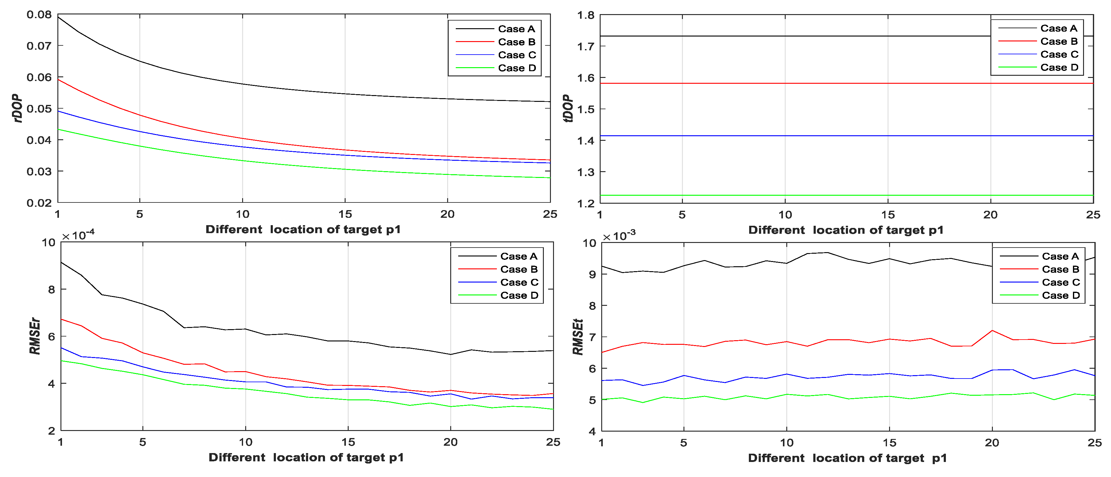
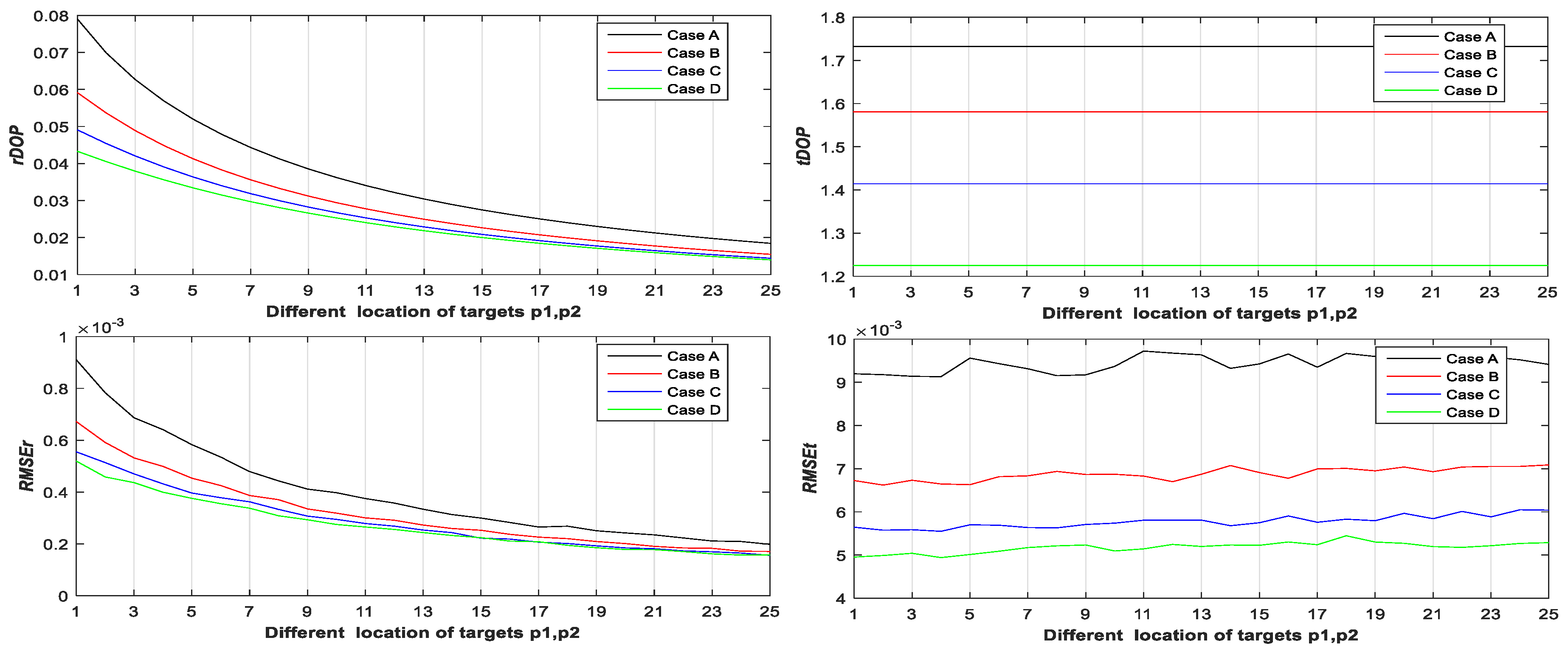
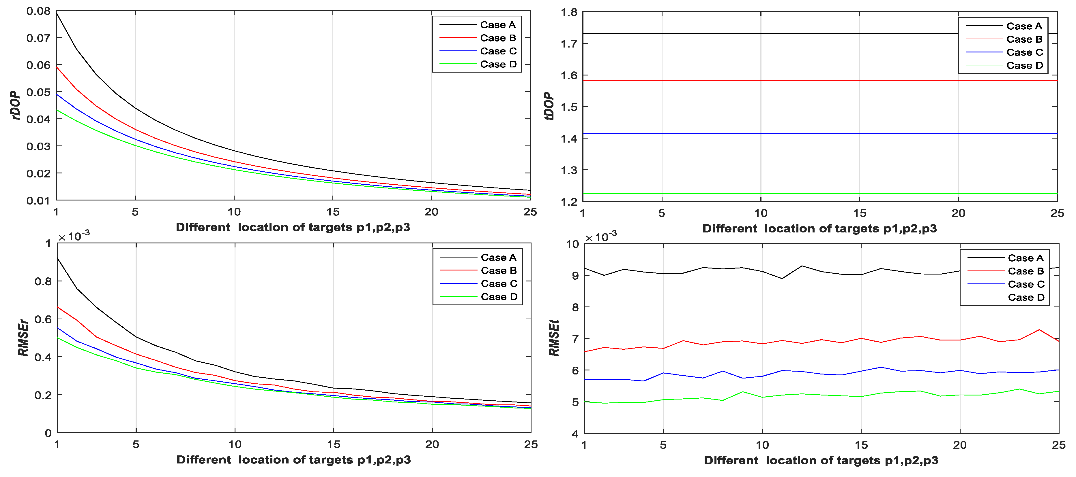
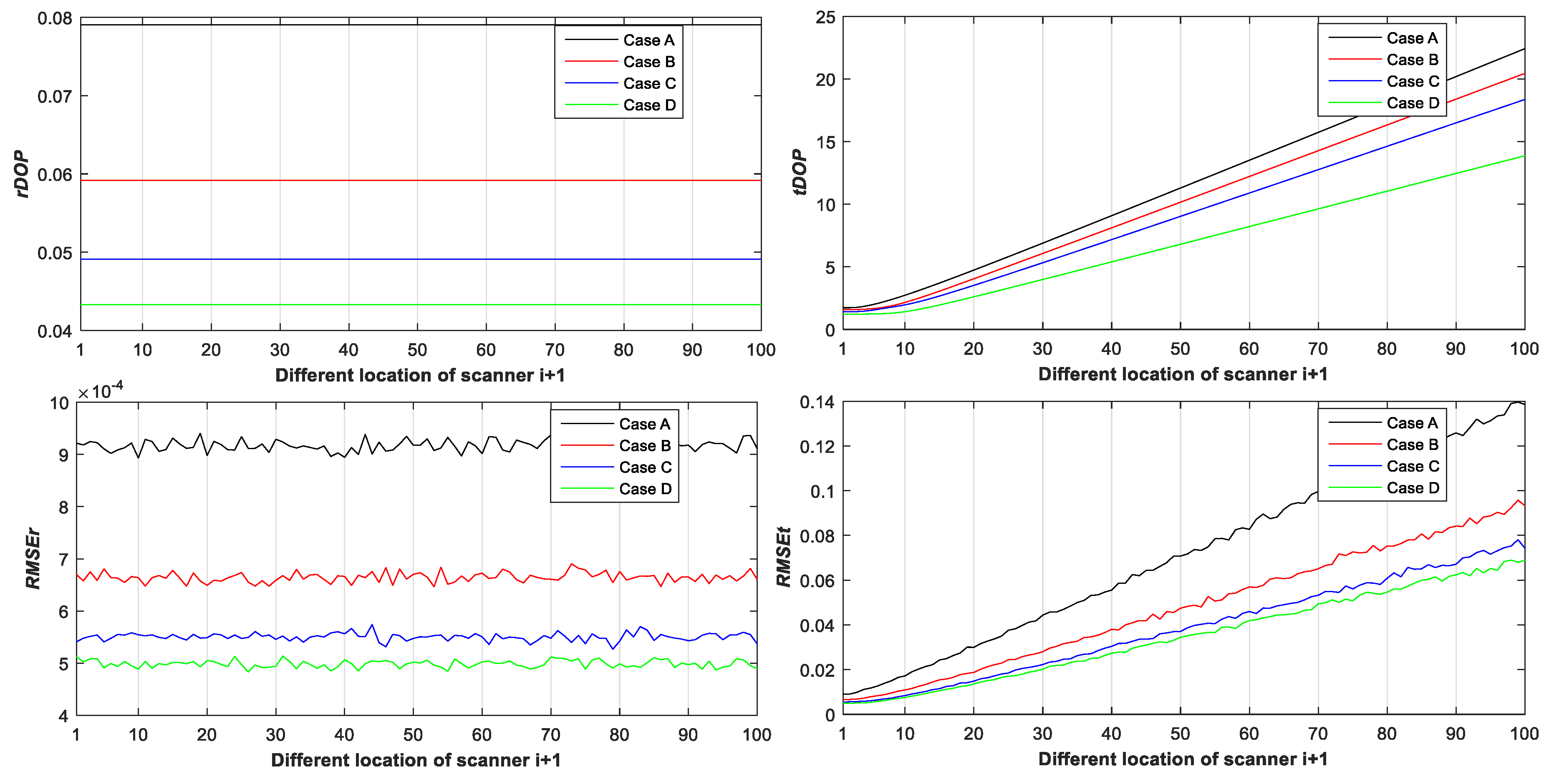
The farther away the location of scanner i + 1 (with respect to different $T_0$), the greater the $tDOP$ and $RMS{E}_t$ in Figure 6;

(c)

When the number and position of targets change, but the location of the scanner is unchanged, the value of $tDOP$ is a constant, the $RMS{E}_t$ is around a constant, and different numbers of targets (with respect to Case A, B, C, and D) have different constant valued of $tDOP$ and $RMS{E}_t$; the more targets (with respect to Case A, B, C, and D), the smaller the $tDOP$ and $RMS{E}_t$ (see Figure 3, Figure 4 and Figure 5);

(d)

The change of $rDOP$ is also basically the same as the change of $RMS{E}_r$; the size of $rDOP$ and $RMS{E}_r$ is related to the number and position of targets (see Figure 3, Figure 4 and Figure 5), not the location of scanner i + 1 (see Figure 6, Figure 7 and Figure 8);

(e)

The more dispersive the targets (with respect to different locations of targets ${\tilde{p}}_1^i,{\tilde{p}}_2^i,{\tilde{p}}_3^i$), the smaller the $rDOP$ and $RMS{E}_r$ in Figure 3, Figure 4 and Figure 5;

(f)

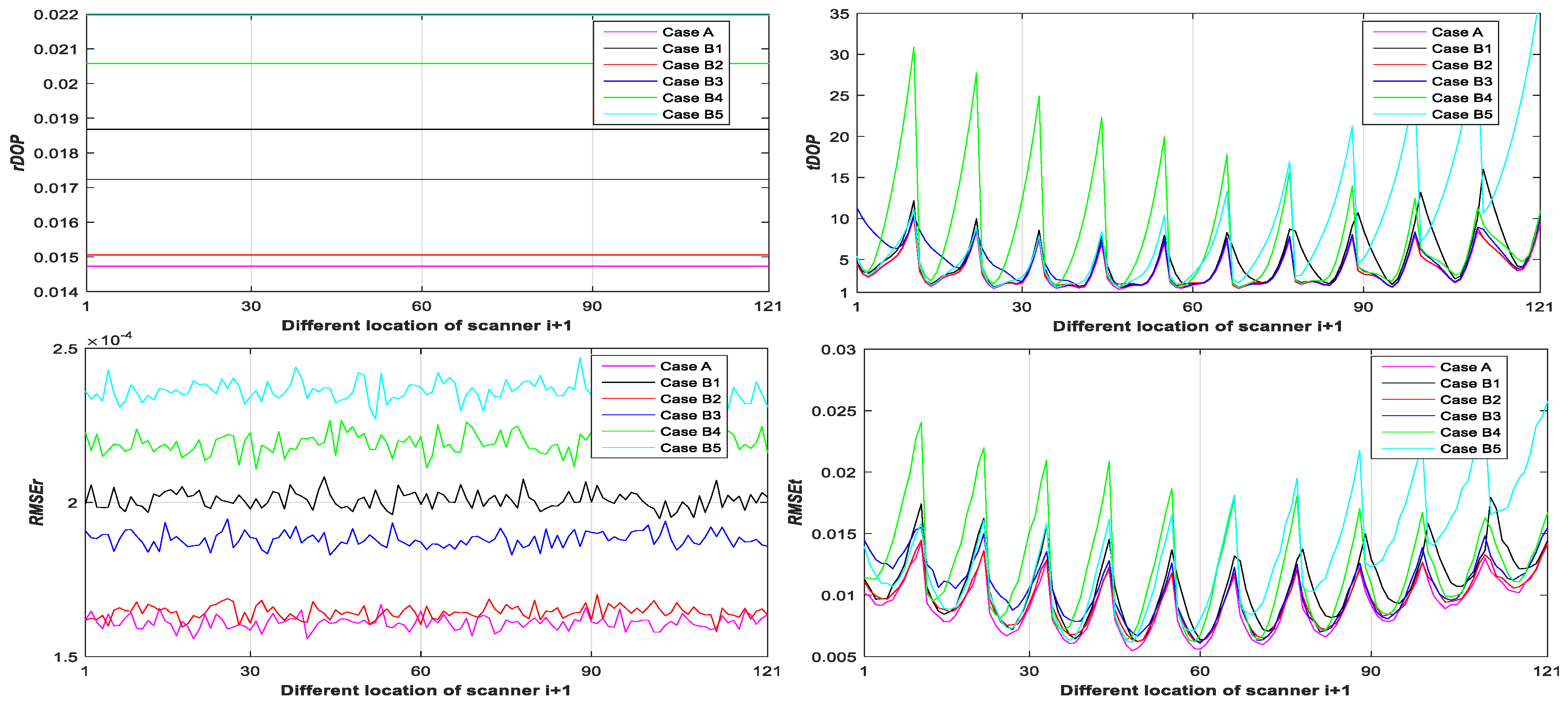
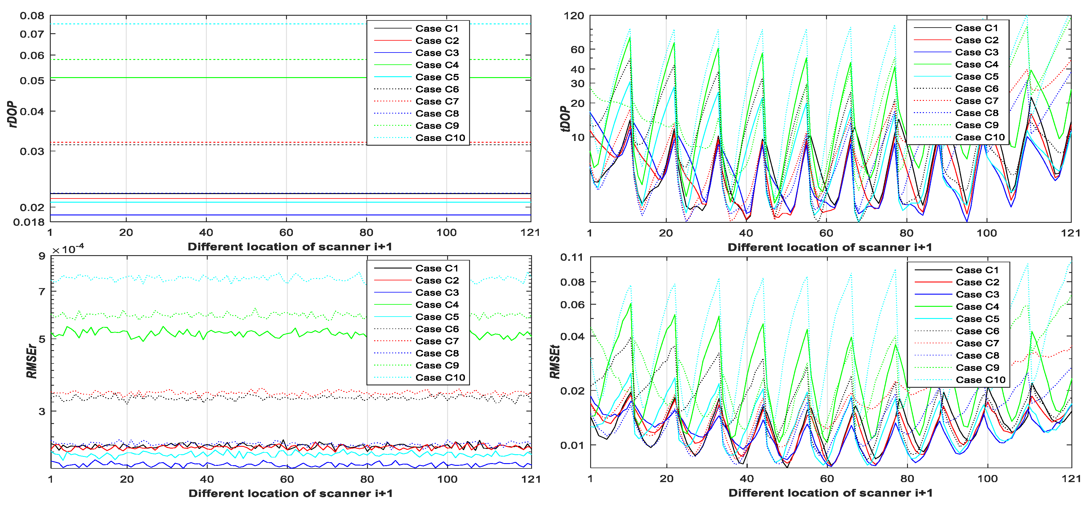
When the location of the scanner changes, but the number and position of targets are unchanged, the value of $rDOP$ is a constant, the $RMS{E}_r$ is around a constant, and different numbers of targets (with respect to Case A, B, C, D, A1, B1–5, and C1–10) have different constant values of $rDOP$ and $RMS{E}_r$; the more targets there are (with respect to Case A, B, C, D, A1, B1–5, and C1–10), the smaller the $rDOP$ and $RMS{E}_r$ (see Figure 6, Figure 7 and Figure 8);

(g)

The differences between the $RMS{E}_t$ and the $RMS{E}_t$ minimum values in cases A1, B1–5, and C1–10 with the minimum $tDOP$ are −0.5, −1.6, −1.8, 0.9, −2, −1.7, −1.5, −1.8, −2.1, −1.5, −1.5, −1.6, −1.3, −1.5, −2.0, and −0.8 mm, respectively, which are all less than $0.5{\sigma }_0$ (half the observation variance, 2.5 mm), so we can use the $RMS{E}_t$ minimum value with the minimum $tDOP$ to represent the $RMS{E}_t$ minimum value;

(h)

We can use $rDOP$ and $tDOP$ to assess the impact of the targets’ geometry distribution on the rotation parameters and translation parameters, respectively, and use $rDOP$ and $tDOP$ to help determine the optimal placement location of targets (with respect to the minimum $rDOP$) and the best location of scanner i + 1 (with respect to the minimum $tDOP$).

5. Conclusions

This research proposes a new evaluation model of TGD (namely, $rDOP$ and $tDOP$) for the first time, and quantitatively verifies that the model can be used to assess the impact of TGD on the registration precision by experiments, which show that “the change of $rDOP$/$tDOP$ is basically the same as the change of the registration precision”. In addition, this research also mathematically proves the existing experiences of TGD by the proposed model, such as “The more targets, the higher the registration precision (corresponding to the smaller $rDOP$ and $tDOP$)”, “The best setting position of the Scanner i + 1 is the barycenter of all targets (corresponding to the minimum $tDOP$ value)”, “The more dispersive the targets, the higher the registration precision (corresponding to the smaller $rDOP$ values)”, “The targets will be not too close to a straight line where bigger $rDOP$ exists”, and “The targets will be not too close on the same plane where bigger $tDOP$ exists”.

If the targets are considered as control points or satellites, we can use the model to help design the optimal control network in engineering surveying and geodetic surveying or the optimal satellite constellation in GNSS. Therefore, we conclude that the proposed $rDOP$ and $tDOP$ model can be considered a unified evaluation model of the TGD, control point distribution, and satellite constellation.

However, it should be noted that “we only theoretically analyze the equal weight model of $rDOP$ and $tDOP$”, “we also do not use the real TLS field data collection and the actual cases to analyze the application effect of the $rDOP$ and $tDOP$ model”, “the experiments do not consider targets’ positioning precision that are affected by many factors (such as the height of scanner/targets, scanning distance, incident angel, material type of targets, etc. [28])”, and “our experiments do not consider other applications such as the engineering surveying, the geodetic surveying, aerial photogrammetry and so on”. In the future, we will conduct more experiments and simulations to verify our model’s applications.

References

1. Deng, F. Registration Between Multiple Laser Scanner Data Sets, Laser Scanning, Theory and Application; Wang, C.C., Ed.; IntechOpen: London, UK, 2011; pp. 449–472. ISBN 978-953-307-205-0. Available online: http://www.intechopen.com/books/laser-scanning-theory-and-applications/registratioin-between-multiple-laser-scanner-data-sets (accessed on 26 April 2011).
2. Reshetyuk, Y. Self-Calibration and Direct Georeferencing in Terrestrial Laser Scanning. Ph.D. Thesis, Royal Institute of Technology, Stockholm, Sweden, 2009. [Google Scholar]
3. Yang, R.H.; Meng, X.L.; Yao, Y.B.; Chen, B.Y.; You, Y.S.; Xiang, Z.J. An analytical approach to evaluate point cloud registration error utilizing targets. ISPRS J. Photogramm. Remote Sens. 2018, 142, 48–56. [Google Scholar] [CrossRef]
4. Sharp, G.C.; Lee, S.W.; Wehe, D.K. Multiview registration of 3D scenes by minimizing error between coordinate frames. IEEE Trans. Pattern Anal. Mach. Intell. 2004, 26, 1037–1050. [Google Scholar] [CrossRef]
5. Eggert, D.W.; Lorusso, A.; Fisher, R.B. Estimating 3-D rigid body transformations: A comparison of four major algorithms. Mach. Vis. Appl. 1997, 9, 272–290. [Google Scholar] [CrossRef]
6. Yao, J.L.; Han, B.M.; Yang, Y.X. Research on registration of ground lidar range images. Geomat. Inf. Sci. Wuhan Univ. 2006, 31, 12–1119. [Google Scholar]
7. Cheng, L.; Chen, S.; Liu, X.Q.; Xu, H.; Wu, Y.; Li, M.C.; Chen, Y.M. Registration of laser scanning point clouds: A review. Sensors 2018, 18, 1641. [Google Scholar] [CrossRef] [PubMed] [Green Version]
8. Flores-Fuentes, W.; Rivas-Lopez, M.; Sergiyenko, O.; Gonzalez-Navarro, F.F.; Rivera-Castillo, J.; Hernandez-Balbuena, D.; Rodríguez-Quiñonez, J.C. Combined application of power spectrum centroid and support vector machines for measurement improvement in optical scanning systems. Signal Process. 2014, 98, 37–51. [Google Scholar] [CrossRef]
9. Rodríguez-Quiñonez, J.C.; Sergiyenko, O.; Flores-Fuentes, W.; Rivera-Castillo, J.; Hernandez-Balbuena, D.; Rascón, R.; Mercorelli, P. Improve a 3D distance measurement accuracy in stereo vision systems using optimization methods’ approach. Opto-Electron. Rev. 2017, 25, 24–32. [Google Scholar] [CrossRef]
10. Janßen, J.; Medic, T.; Kuhlmann, H.; Holst, C. Decreasing the uncertainty of the target center estimation at terrestrial laser scanning by choosing the best algorithm and by improving the target design. Remote Sens. 2019, 11, 845. [Google Scholar] [CrossRef] [Green Version]
11. Wang, G.L. Research on Registration of Ground Lidar Range Images. Master’s Thesis, Beijing University of Civil Engineering and Architecture, Beijing, China, 2006. [Google Scholar]
12. Fan, L.; Smethurst, J.A.; Atkinson, P.M.; Powrie, W. Error in target-based georeferencing and registration in terrestrial laser scanning. Comput. Geosci. 2015, 83, 54–64. [Google Scholar] [CrossRef] [Green Version]
13. Pan, L.X.L. Research on Some Problems of Point Cloud. Master’s Thesis, Chongqing University, Chongqing, China, 2018. [Google Scholar]
14. Gordon, S.J.; Lichti, D.D. Terrestrial laser scanners with a narrow field of view: The effect on 3D resection solutions. Surv. Rev. 2004, 37, 292–468. [Google Scholar] [CrossRef]
15. Harvey, B.R. Registration and transformation of multiple site terrestrial laser scanning. Geomat. Res. Australas. 2004, 80, 33–50. [Google Scholar]
16. Li, Z.C. Research on the Algorithm and Accuracy of Coordinate Conversion. Master’s Thesis, Kuming University of Science and Technology, Kuming, China, 2015. [Google Scholar]
17. Liu, K.; Liao, Z.P.; Ding, M.Q.; Xiang, Y.; Cai, C.G. Effects on accuracy of point cloud registration by target setting between the stations. Geotech. Investig. Surv. 2016, 4, 55–58, 67. [Google Scholar]
18. Wang, Y.C.; Hu, W.S. Influence caused by public point selection on accuracy of coordinate conversion. Mod. Surv. Mapp. 2008, 31, 5–15. [Google Scholar]
19. Zhao, B.F.; Zhang, X.; Jiang, T.C. Effect of coordinate conversion model and the selected common points on the accuracy of conversion results. J. Huaihai Inst. Technol. Nat. Sci. Ed. 2009, 18, 4–56. [Google Scholar]
20. Zhang, H.L.; Lin, J.R.; Zhu, J.G. Three-dimensional coordinate transformation accuracy and its influencing factors. Opto-Electron. Eng. 2012, 39, 10–31. [Google Scholar]
21. Bornaz, L.; Lingus, A.; Rinaudo, F. Multiple Scan Registration in LiDAR Close-Range Applications. 2003. Available online: https://pdfs.semanticscholar.org/ce10/a74f8de40df362c8a9cc8f54fa0e6484b4f4.pdf (accessed on 18 January 2020).
22. Li, Z.H.; Huang, J.S. GPS Surveying Data Processing, 2nd ed.; Wuhan University press: Wuhan, China, 2010; pp. 160–162. [Google Scholar]
23. Yang, R.H. Research on Point Cloud Angular Resolution and Processing Model of Terrestrial Laser Scanning. Ph.D. Thesis, Wuhan University, Wuhan, China, 2011. [Google Scholar]
24. Cui, X.Z.; Yu, Z.S.; Tao, B.Z.; Liu, D.J.; Yu, Z.L.; Sun, H.Y.; Wang, X.Z. Generalized Surveying Adjustment, 2nd ed.; Wuhan University press: Wuhan, China, 2009; pp. 8–9. [Google Scholar]
25. Li, J.W.; Li, Z.H.; Zhou, W.; Si, S.J. Study on the minimum of GDOP in Satellite navigation and its applications. Acta Geodaetica Cartogr. Sin. 2011, 40, 85–88. [Google Scholar]
26. Meng, X.; Roberts, G.W.; Dodson, A.H.; Cosser, E.; Barnes, J.; Rizos, C. Impact of GPS satellite and pseudolite geometry on structural deformation monitoring: Analystical and empirical studies. J. Geod. 2004, 77, 12–822. [Google Scholar] [CrossRef]
27. Yarlagadda, R.; Ali, I.; Dhahir, N.A.; Hershey, J. GPS DOP Metric. IEEE Proc. Radar Sonar Navig. 2000, 147, 5–264. [Google Scholar] [CrossRef]
28. Soudarissanane, S.; Lindenbergh, R.; Menenti, M.; Teunissen, P. Scanning geometry: Influnencing factor on the quanlity of terrestrial laser scanning points. ISPRS J. Photogramm. Remote Sens. 2011, 66, 389–399. [Google Scholar] [CrossRef]
Figure 1. The target geometry of experiment I.
Sensors 20 00555 g001
Figure 2. The target and scanner i + 1 geometry of experiment II.
Sensors 20 00555 g002
Figure 3. r D O P 1 , t D O P 1 , R M S E r , 1 , and R M S E t , 1 of Case A, B, C, and D with respect to one different target.
Sensors 20 00555 g003
Figure 4. r D O P 2 , t D O P 2 , R M S E r , 2 , and R M S E t , 2 of Case A, B, C, and D with respect to two different targets.
Sensors 20 00555 g004
Figure 5. r D O P 3 , t D O P 3 , R M S E r , 3 , and R M S E t , 3 of Case A, B, C, and D with respect to three different targets.
Sensors 20 00555 g005
Figure 6. r D O P 4 , t D O P 4 , R M S E r , 4 , and R M S E t , 4 of Case A, B, C, and D with respect to different Scanner i + 1.
Sensors 20 00555 g006
Figure 7. r D O P 5 , t D O P 5 , R M S E r , 5 , and R M S E t , 5 of Case A and B1–5 with respect to different scanner i + 1.
Sensors 20 00555 g007
Figure 8. r D O P 6 , t D O P 6 , R M S E r , 6 , and R M S E t , 6 of Case C1–10 with respect to different scanner i + 1.
Sensors 20 00555 g008