White-Hat Worm to Fight Malware and Its Evaluation by Agent-Oriented Petri Nets †


Abstract
1. Introduction
2. Related Work
2.1. Mirai and Hajime
2.2. PN and Modeling
2.3. Simulation Evaluation
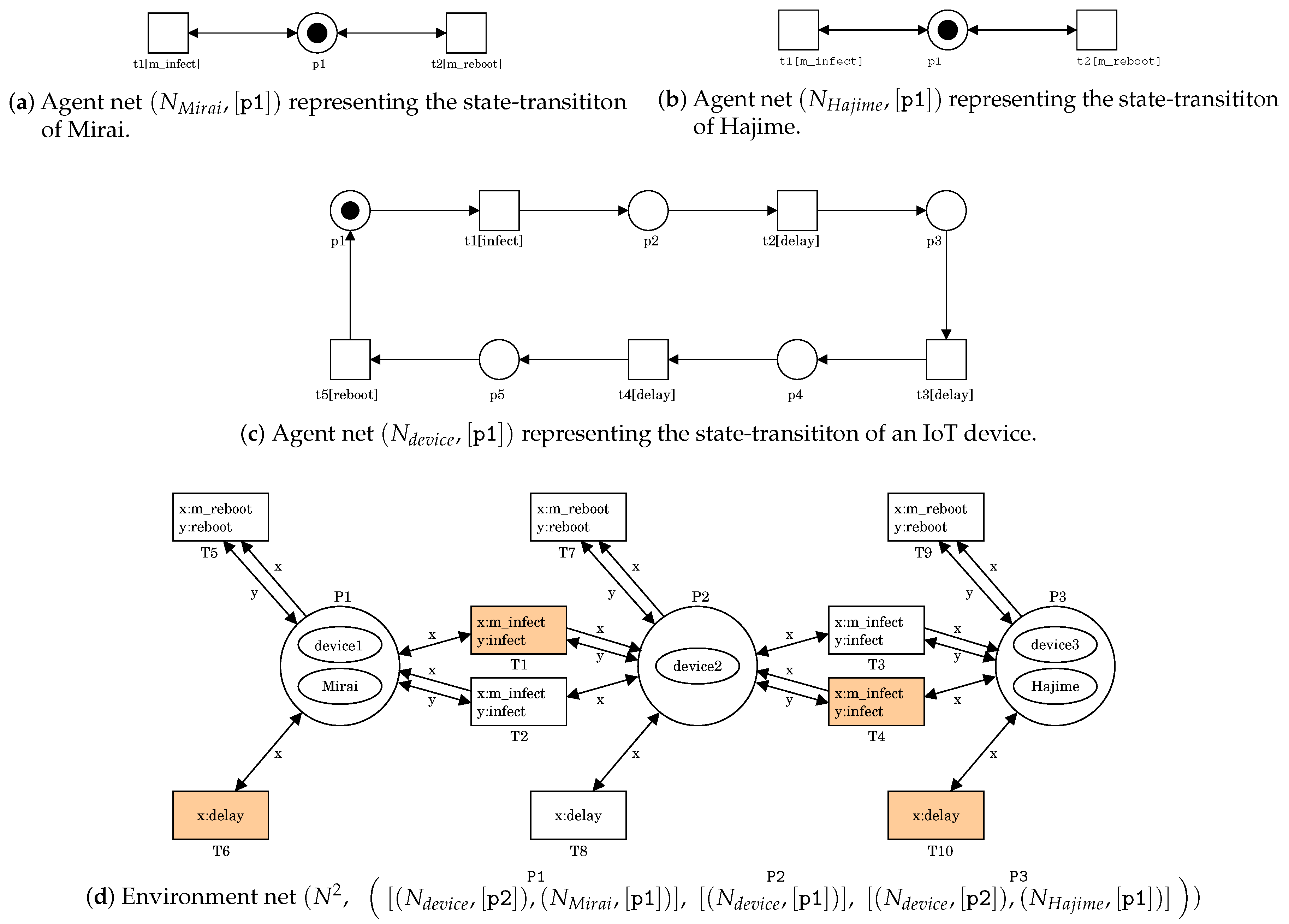
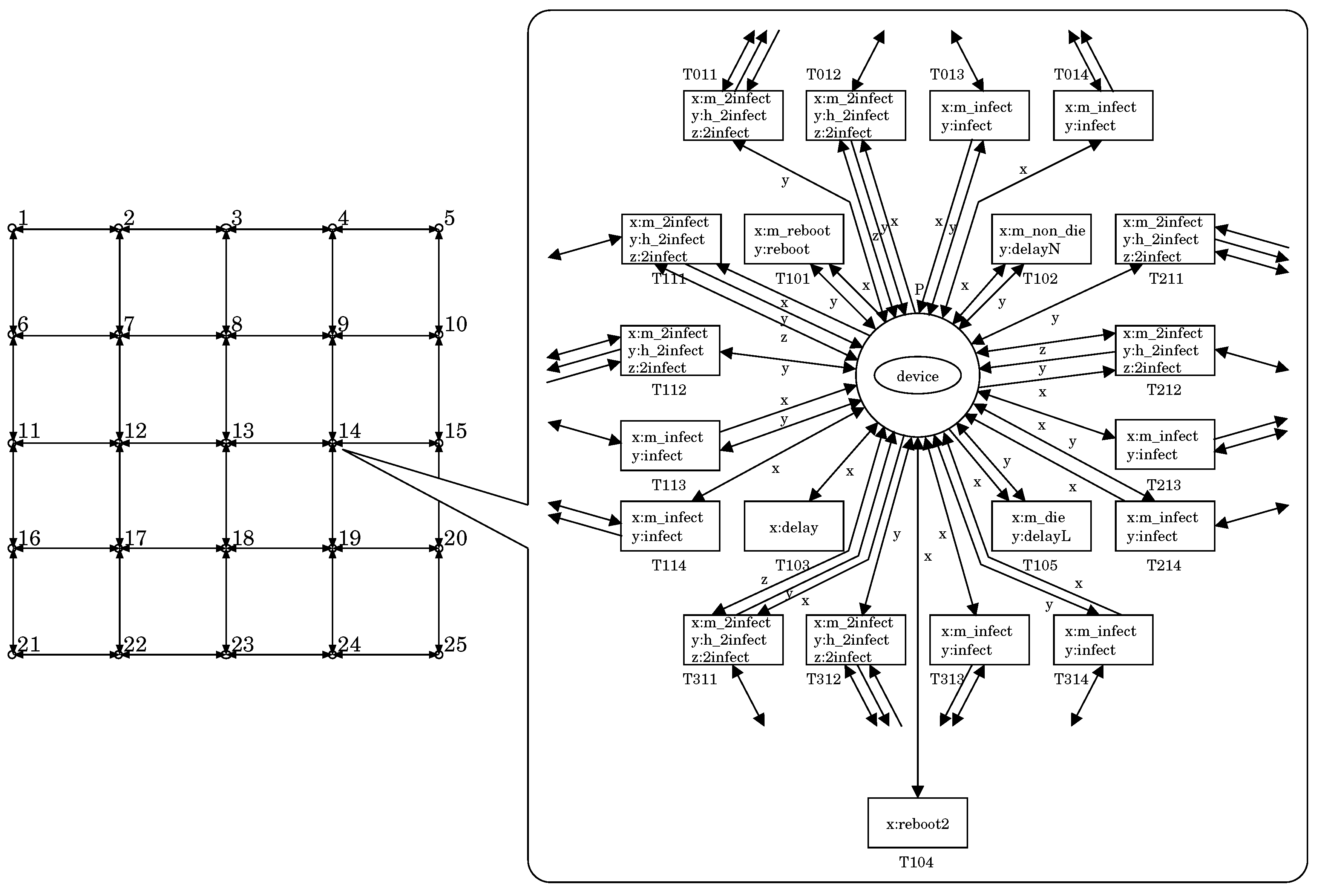
- For T1, x:m_infect and y:infect can be respectively bounded with t1 in at P1 and t1 in at P2.
- For T4, x:m_infect and y:infect can be respectively bounded with t1 in at P3 and t1 in at P2.
- For T6, x:delay can be bounded with t2 in at P1.
- For T10, x:delay can be bounded with t2 in at P3.
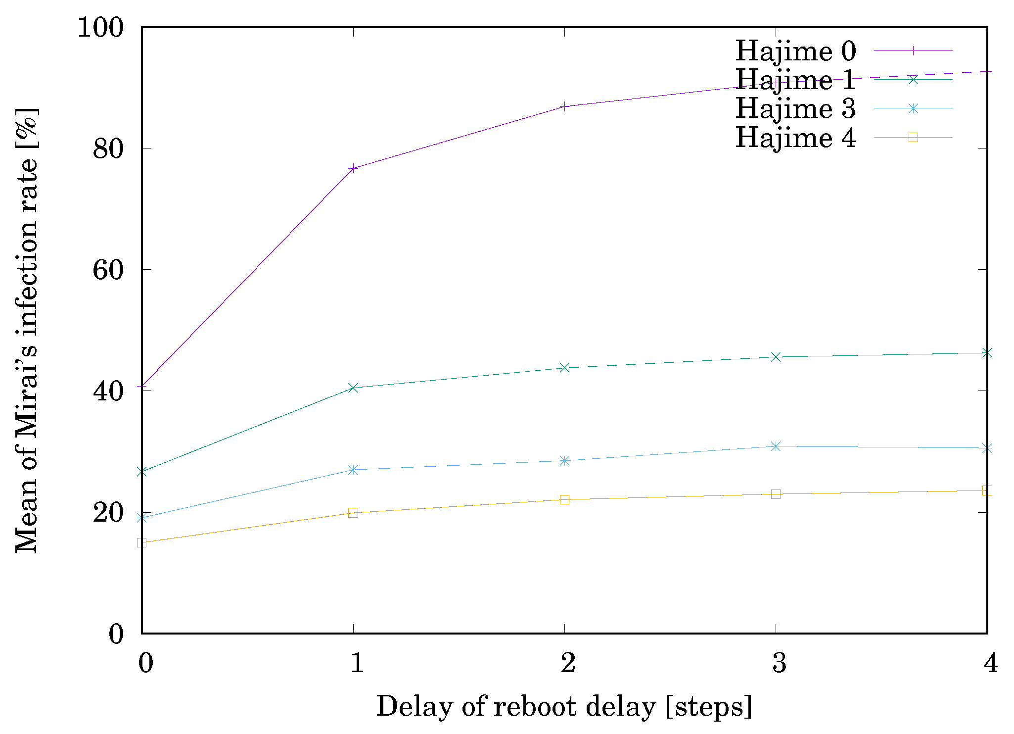
- The delay time until rebooting = 0, 1, 2, 3, or 4 steps.
- The initial number of devices infected by Mirai = 1.
- The initial number of devices infected by Hajime = 0, 1, 2, or 3.
3. White-Hat Worm
3.1. Analysis and Design
3.2. Modeling
3.3. Simulation
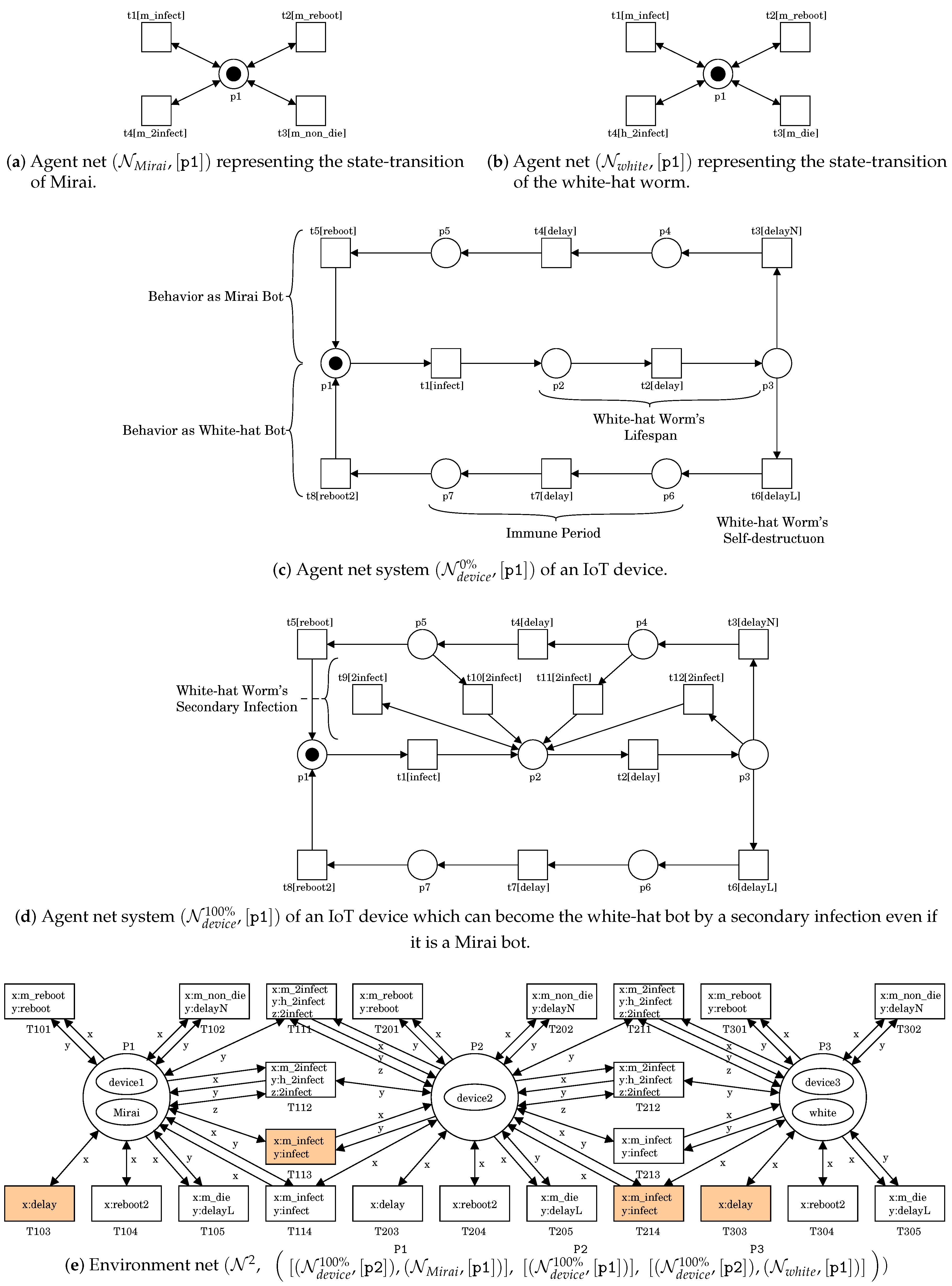
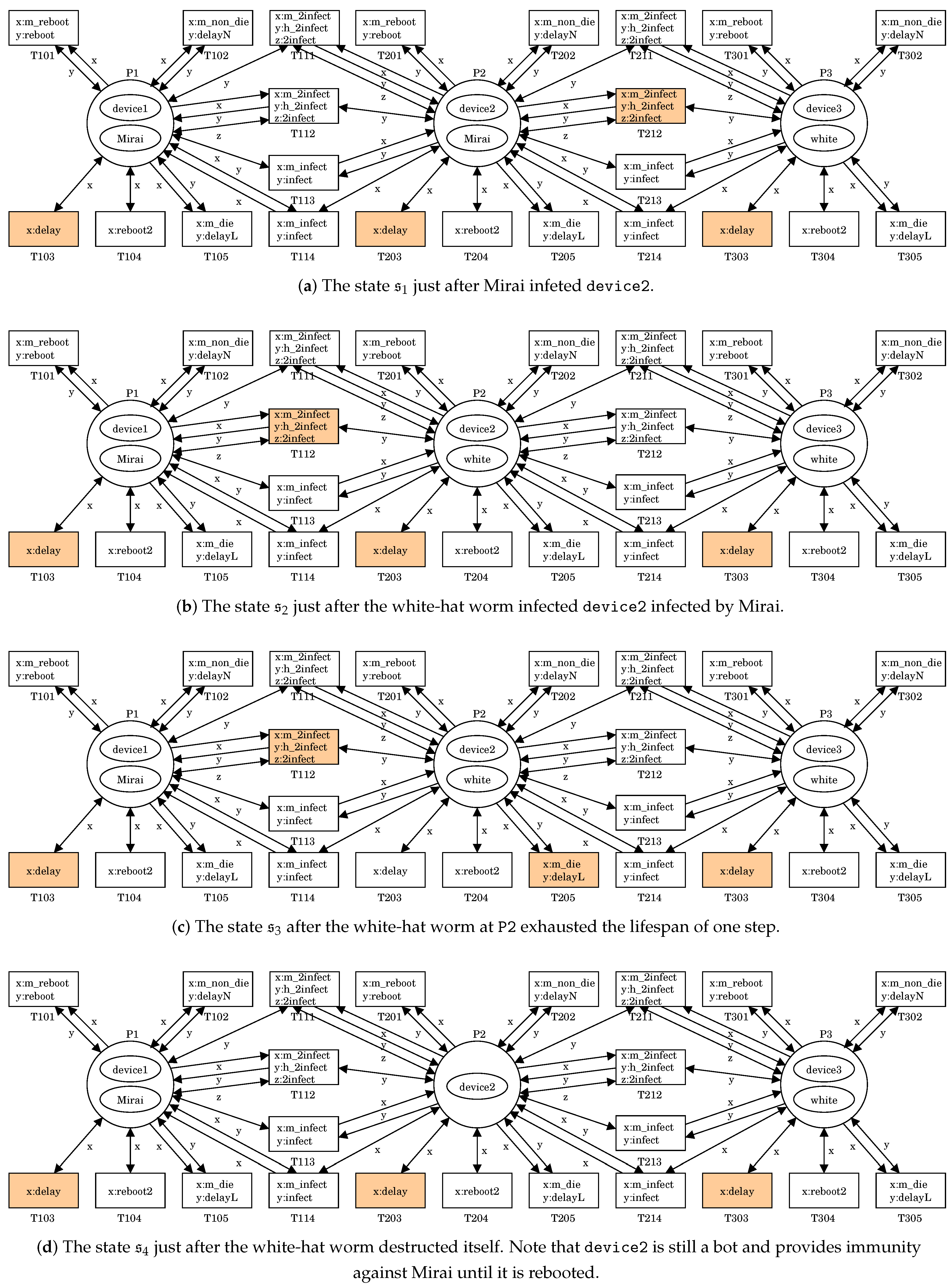
- For T103, T203, or T303, x:delay can be bounded with t2 in .
- For T212, x:m_2infect, y:h_2infect and z:2infect can be respectively bounded with t4 in at P2, t4 in at P3 and t9 in at P2.
- For T103, T203, or T303, x:delay can be bounded with t2 in .
- For T112, x:m_2infect, y:h_2infect and z:2infect can be respectively bounded with t4 in at P1, t4 in at P2 and t9 in at P1.
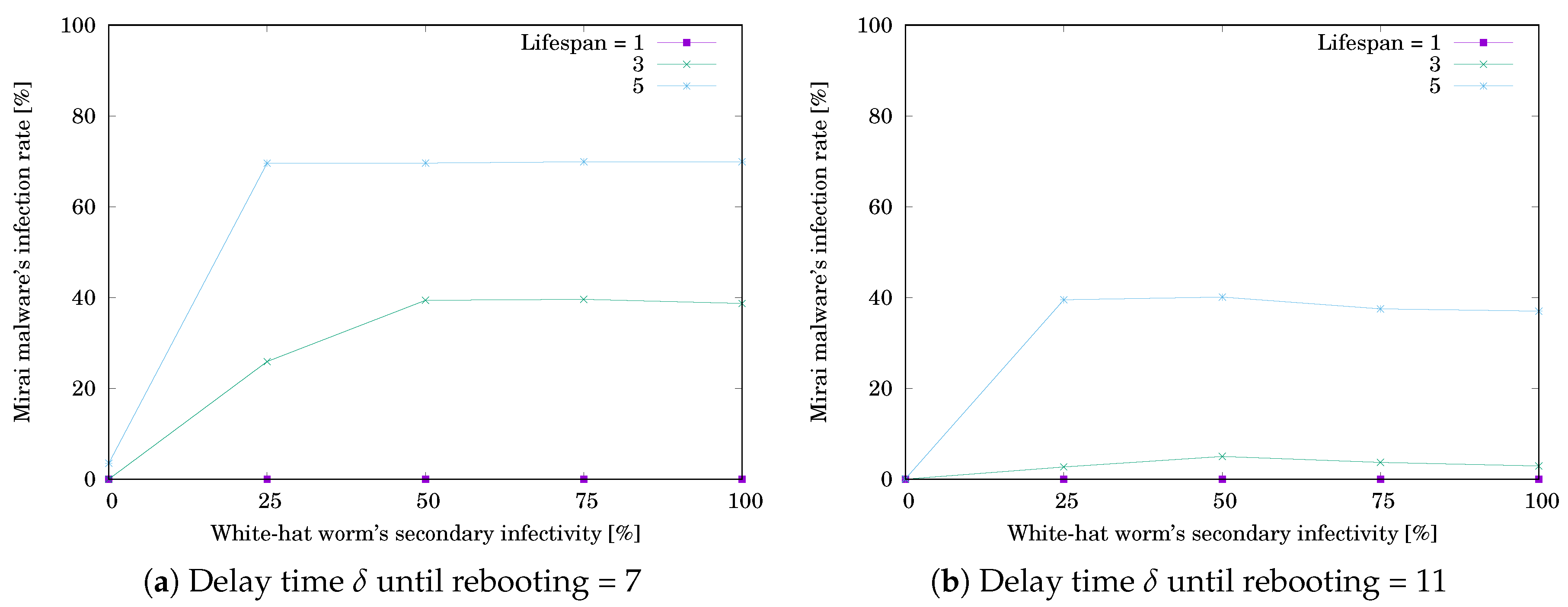
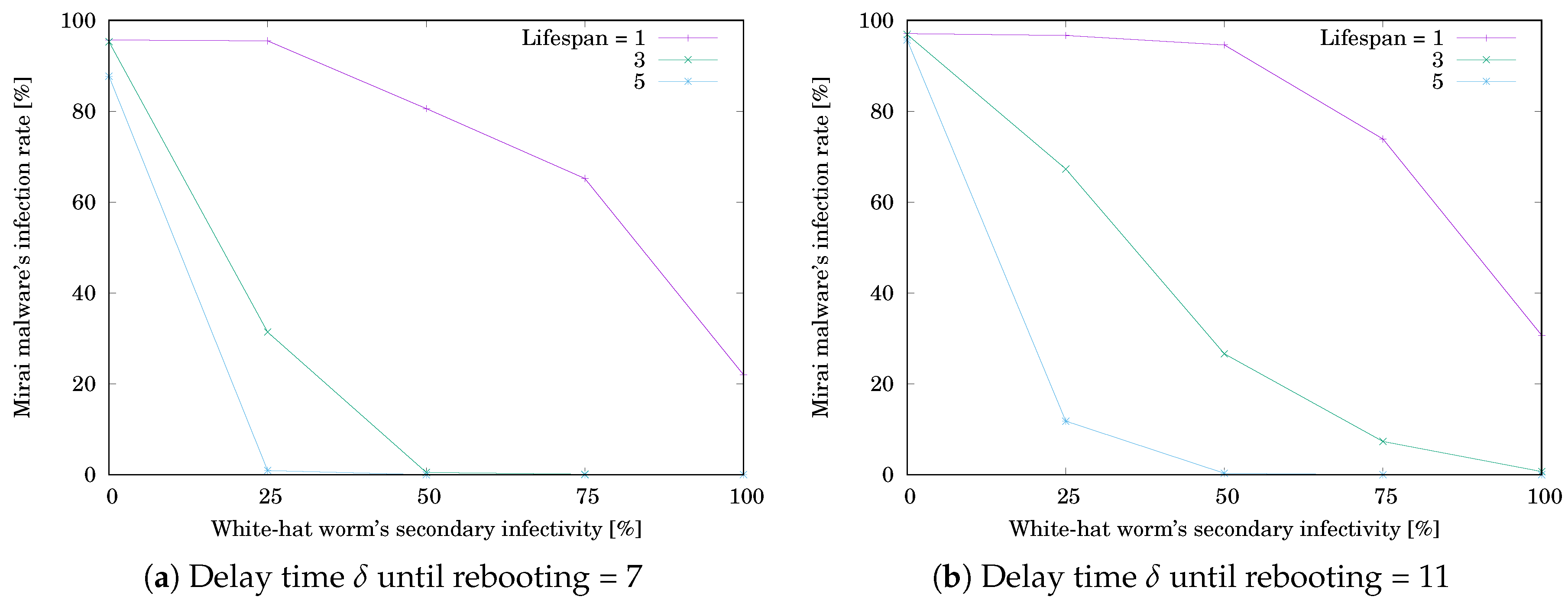
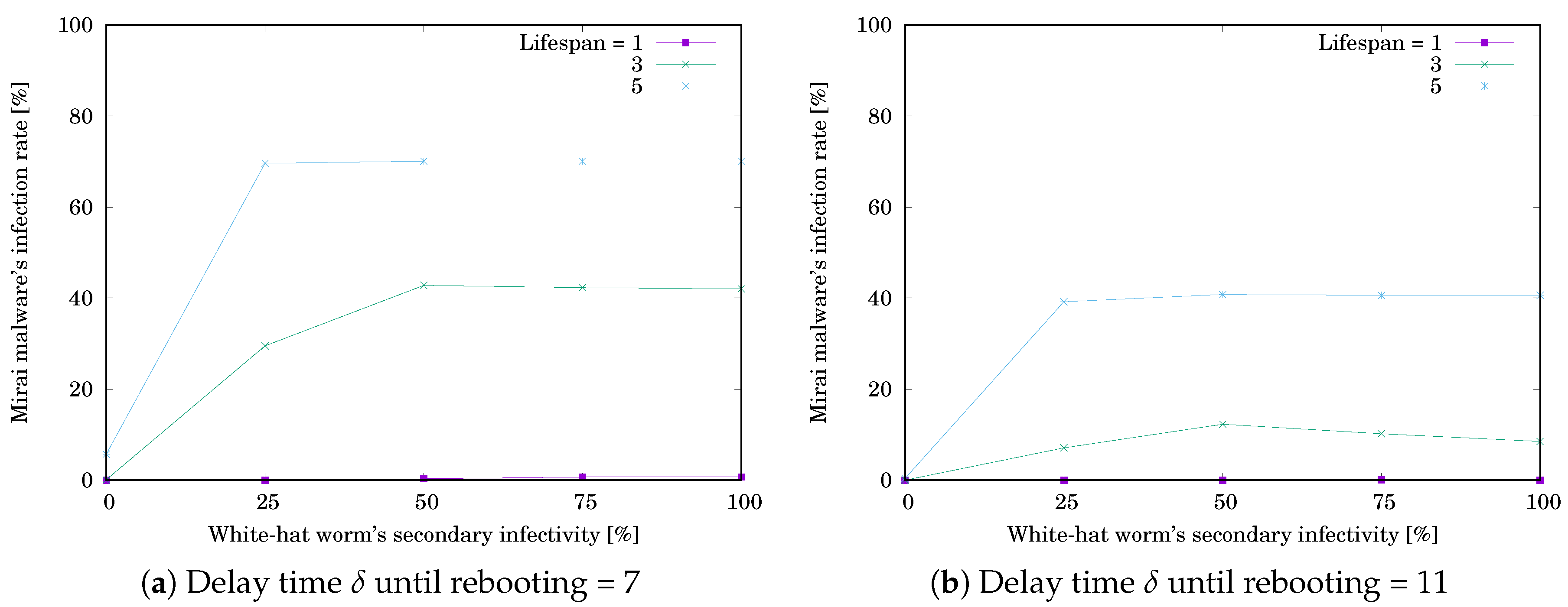
4. Simulation Evaluation
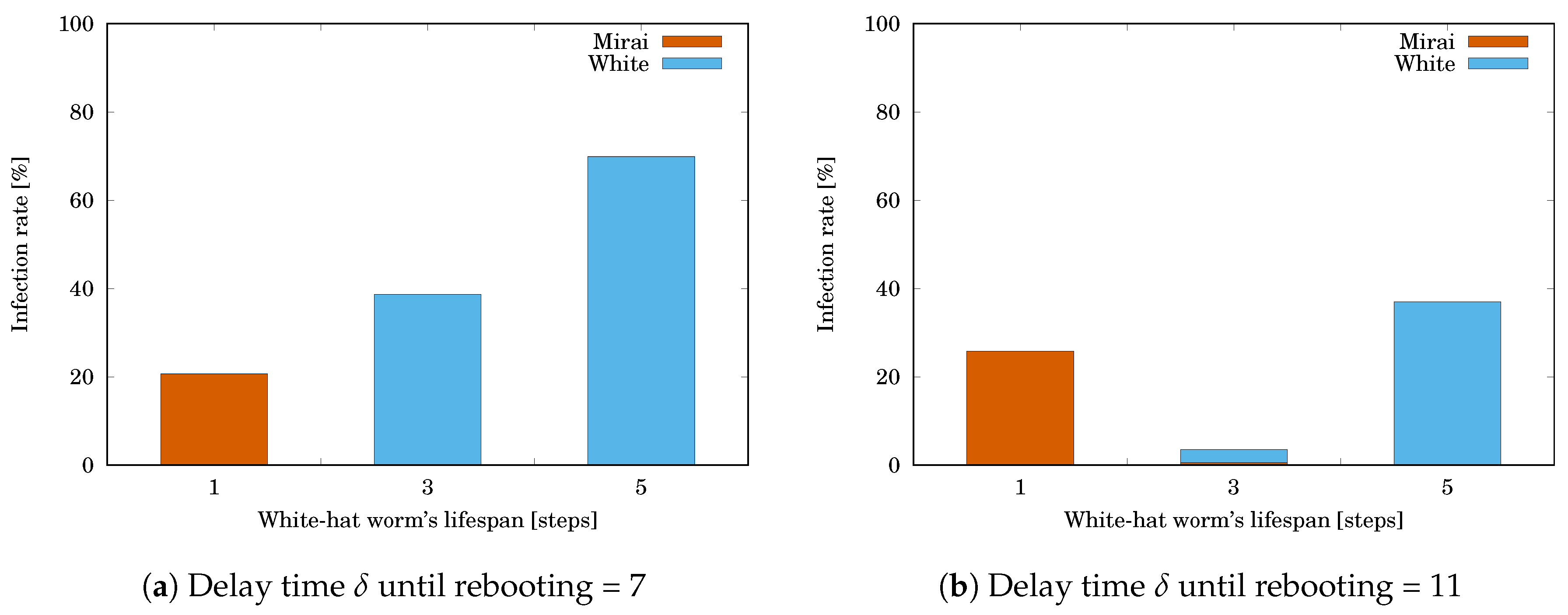
- The delay time until rebooting = 7 or 11 steps,
- The initial number of devices infected by Mirai = 12,
- The initial number of devices infected by the white-hat worm = 5,
- The white-hat worm’s lifespan ℓ = 1, 3, or 5 steps,
- The white-hat worm’s secondary infection possibility = 100%.
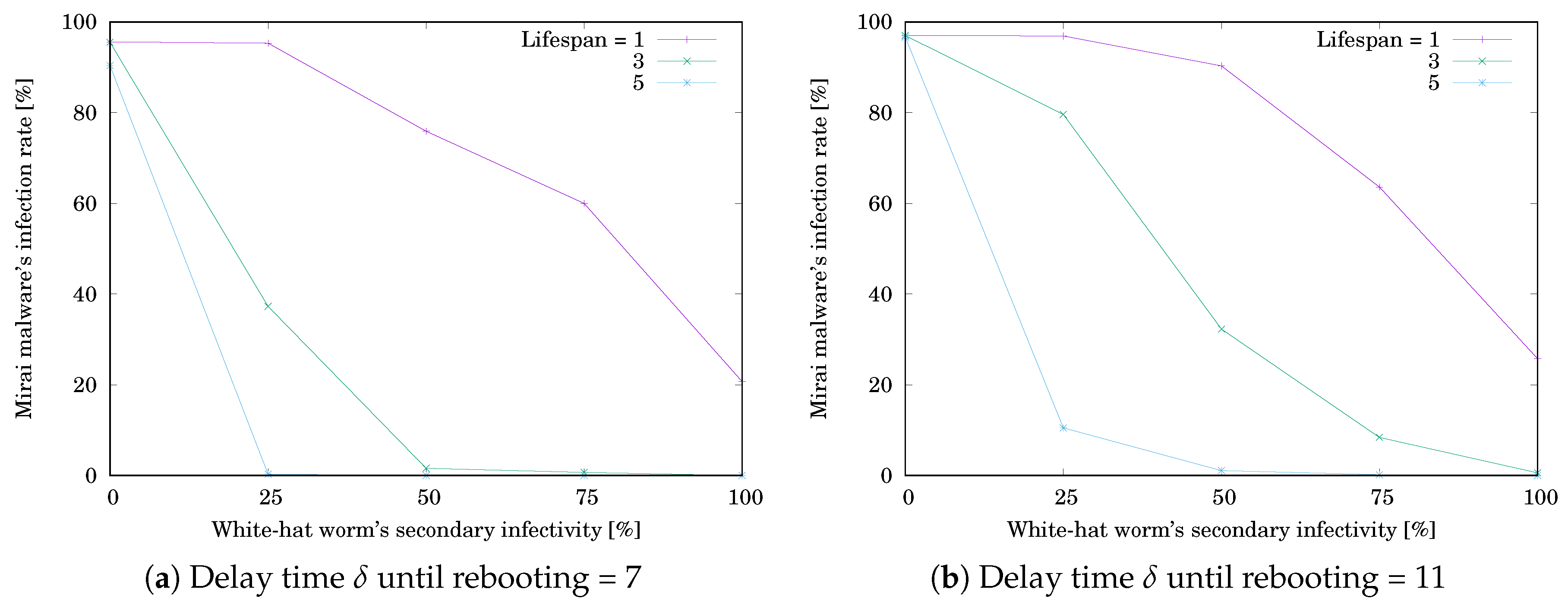
- The white-hat worm’s secondary infection possibility = 0, 25, 50, 75, or 100%
- The initial number of devices infected by Mirai = 18,
- The initial number of devices infected by the white-hat worm = 7.
5. Conclusions
Funding
Conflicts of Interest
References
- Sinaović, H.; Mrdovic, S. Analysis of Mirai malicious software. In Proceedings of the 25th International Conference on Software, Telecommunications and Computer Networks (SoftCOM), Split, Croatia, 21–23 September 2017; pp. 1–5. [Google Scholar]
- Nakao, K. Proactive cyber security response by utilizing passive monitoring technologies. In Proceedings of the 36th IEEE International Conference on Consumer Electronics (ICCE 2018), Las Vegas, NV, USA, 12–14 January 2018. [Google Scholar]
- Kolias, C.; Kambourakis, G.; Stavrou, A.; Voas, J. DDoS in the IoT: Mirai and other botnets. IEEE Comput. 2017, 50, 80–84. [Google Scholar] [CrossRef]
- US Computer Emergency Readiness Team. Heightened DDoS Threat Posed by Mirai and Other Botnets. alert TA16-288A. Available online: Https://www.us-cert.gov/ncas/alerts/TA16-288A (accessed on 29 October 2019).
- Edwards, S.; Profetis, I. Hajime: Analysis of a Decentralized Internet Worm for IoT Devices. Available online: Http://security.rapiditynetworks.com/publications/2016-10-16/Hajime.pdf (accessed on 29 October 2019).
- Tanaka, H.; Yamaguchi, S. On modeling and simulation of the behavior of IoT devices malwares Mirai and Hajime. In Proceedings of the IEEE International Symposium on Consumer Electronics (ISCE), Kuala Lumpur, Malaysia, 14–15 November 2017; pp. 56–60. [Google Scholar]
- Hiraishi, K. A Petri-net-based model for the mathematical analysis of multi-agent systems. IEICE Trans. Fundam. 2001, 84, 2829–2837. [Google Scholar]
- Yamaguchi, S.; Gupta, B.B. Malware Threat in Internet of Things and Its Mitigation Analysis. In Security, Privacy, and Forensics Issues in Big Data; Joshi, R.C., Gupta, B.B., Eds.; Business Science Reference: Hershey, PA, USA, 2019; pp. 363–379. [Google Scholar]
- Bezerra, V.H.; da Costa, V.G.T.; Barbon, J.; Miani, R.S.; Zarpelão, B.B. IoTDS: A One-Class Classification Approach to Detect Botnets in Internet of Things Devices. Sensors 2019, 19, 3188. [Google Scholar] [CrossRef] [PubMed]
- Liu, X.; Du, X.; Zhang, X.; Zhu, Q.; Wang, H.; Guizani, M. Adversarial Samples on Android Malware Detection Systems for IoT Systems. Sensors 2019, 19, 974. [Google Scholar] [CrossRef] [PubMed]
- Ceron, J.M.; Steding-Jessen, K.; Hoepers, C.; Granville, L.Z.; Margi, C.B. Improving IoT Botnet Investigation Using an Adaptive Network Layer. Sensors 2019, 19, 727. [Google Scholar] [CrossRef] [PubMed]
- Grange, W. Hajime Battles Mirai for Control of the Internet of Things. Available online: Https://www.symantec.com/connect/blogs/Hajime-worm-battles-Mirai-control-internet-things (accessed on 29 October 2019).
- Molesky, M.J.; Cameron, E.A. Internet of Things: An Analysis and Proposal of White Worm Technology. In Proceedings of the 37th IEEE International Conference on Consumer Electronics (ICCE 2019), Las Vegas, NV, USA, 11–13 January 2019. [Google Scholar]
- Yamaguchi, S.; Tanaka, H.; Bin Ahmadon, M.A. Modeling and Evaluation of Mitigation Methods against IoT Malware Mirai with Agent-Oriented Petri Net PN2. Int. J. Internet Things Cyber Assur. 2019. [Google Scholar] [CrossRef]
- Nakahori, K.; Yamaguchi, S. A support tool to design IoT services with NuSMV. In Proceedings of the 35th IEEE International Conference on Consumer Electronics (ICCE 2017), Las Vegas, NV, USA, 8–10 January 2017; pp. 84–87. [Google Scholar]
- Yamaguchi, S.; Bin Ahmadon, M.A.; Ge, Q.W. Introduction of Petri Nets: Its Applications and Security Challenges. In Handbook of Research on Modern Cryptographic Solutions for Computer and Cyber Security; Gupta, B.B., Agrawal, D.P., Yamaguchi, S., Eds.; IGI Publishing: Hershey, PA, USA, 2016; pp. 145–179. [Google Scholar]
- García-Magariño, I.; Gómez-Rodríguez, A.; González-Moreno, J.C.; Palacios-Navarro, G. PEABS: A Process for developing Efficient Agent-Based Simulators. Eng. Appl. Artif. Intell. 2015, 46 Pt A, 104–112. [Google Scholar] [CrossRef]
- García-Magariño, I.; Lacuesta, R. ABS-TrustSDN: An Agent-Based Simulator of Trust Strategies in Software-Defined Networks. Secur. Commun. Netw. 2017, 3, 1–9. [Google Scholar] [CrossRef]
- Tanaka, H.; Yamaguchi, S.; Mikami, M. Quantitative Evaluation of Hajime with Secondary Infectivity in Response to Mirai’s Infection Situation. In Proceedings of the 8th IEEE Global Conference on Consumer Electronics (GCCE 2019), Osaka, Japan, 15–18 October 2019; pp. 985–988. [Google Scholar]
- Moffitt, T. Source Code for Mirai IoT Malware Released. Available online: Https://www.webroot.com/blog/2016/10/10/source-code-Mirai-iot-malware-released/ (accessed on 4 November 2019).
- Yamaguchi, S. Botnet Defense System: Concept and Basic Strategy. In Proceedings of the 38th IEEE International Conference on Consumer Electronics (ICCE 2020), Las Vegas, NV, USA, 4–6 January 2020. [Google Scholar]


| The Initial Number | The Delay Time until Rebooting | ||||
|---|---|---|---|---|---|
| of Hajime | 0 | 1 | 2 | 3 | 4 |
| 0 | 40.8% | 76.7% | 86.9% | 90.8% | 92.7% |
| 1 | 26.7% | 40.5% | 43.8% | 45.6% | 46.3% |
| 2 | 19.1% | 27.0% | 28.5% | 30.9% | 30.6% |
| 3 | 15.0% | 19.9% | 22.1% | 23.0% | 23.6% |
| (a) | ||
|---|---|---|
| Lifespan ℓ | ||
| 1 | 20.7% | 0.0% |
| 3 | 0.0% | 38.7% |
| 5 | 0.0% | 69.9% |
| (b) | ||
| Lifespan ℓ | ||
| 1 | 25.8% | 0.0% |
| 3 | 0.6% | 2.9% |
| 5 | 0.0% | 37.0% |
| (a) | |||||
|---|---|---|---|---|---|
| Lifespan ℓ | White-Hat Worm’s Secondary Infectivity | ||||
| 0% | 25% | 50% | 75% | 100% | |
| 1 | 95.6% | 95.3% | 75.9% | 60.0% | 20.7% |
| 3 | 95.5% | 37.3% | 1.6% | 0.7% | 0.0% |
| 5 | 90.4% | 0.3% | 0.0% | 0.0% | 0.0% |
| (b) | |||||
| Lifespan ℓ | White-Hat Worm’s Secondary Infectivity | ||||
| 0% | 25% | 50% | 75% | 100% | |
| 1 | 97.0% | 96.9% | 90.3% | 63.6% | 25.8% |
| 3 | 97.0% | 79.6% | 32.3% | 8.4% | 0.6% |
| 5 | 96.7% | 10.5% | 1.1% | 0.2% | 0.0% |
| (a) | |||||
|---|---|---|---|---|---|
| Lifespan ℓ | White-Hat Worm’s Secondary Infectivity | ||||
| 0% | 25% | 50% | 75% | 100% | |
| 1 | 0.0% | 0.0% | 0.0% | 0.0% | 0.0% |
| 3 | 0.0% | 25.9% | 39.4% | 39.6% | 38.7% |
| 5 | 3.5% | 69.6% | 69.6% | 69.9% | 69.9% |
| (b) | |||||
| Lifespan ℓ | White-Hat Worm’s Secondary Infectivity | ||||
| 0% | 25% | 50% | 75% | 100% | |
| 1 | 0.0% | 0.0% | 0.0% | 0.0% | 0.0% |
| 3 | 0.0% | 2.7% | 5.0% | 3.7% | 2.9% |
| 5 | 0.1% | 39.5% | 40.1% | 37.5% | 37.0% |
| (a) | |||||
|---|---|---|---|---|---|
| Lifespan ℓ | White-Hat Worm’s Secondary Infectivity | ||||
| 0% | 25% | 50% | 75% | 100% | |
| 1 | 95.7% | 95.5% | 80.6% | 65.2% | 22.0% |
| 3 | 95.3% | 31.4% | 0.5% | 0.1% | 0.0% |
| 5 | 87.7% | 0.9% | 0.0% | 0.0% | 0.0% |
| (b) | |||||
| Lifespan ℓ | White-Hat Worm’s Secondary Infectivity | ||||
| 0% | 25% | 50% | 75% | 100% | |
| 1 | 97.1% | 96.7% | 94.6% | 73.9% | 30.7% |
| 3 | 96.9% | 67.3% | 26.6% | 7.3% | 0.7% |
| 5 | 95.7% | 11.8% | 0.3% | 0.0% | 0.0% |
| (a) | |||||
|---|---|---|---|---|---|
| Lifespan ℓ | White-Hat Worm’s Secondary Infectivity | ||||
| 0% | 25% | 50% | 75% | 100% | |
| 1 | 0.0% | 0.0% | 0.3% | 0.7% | 0.7% |
| 3 | 0.1% | 29.5% | 42.8% | 42.3% | 42.0% |
| 5 | 5.7% | 69.6% | 70.1% | 70.1% | 70.1% |
| (b) | |||||
| Lifespan ℓ | White-Hat Worm’s Secondary Infectivity | ||||
| 0% | 25% | 50% | 75% | 100% | |
| 1 | 0.0% | 7.1% | 12.3% | 0.1% | 0.0% |
| 3 | 0.0% | 0.2% | 0.4% | 10.2% | 8.5% |
| 5 | 0.4% | 39.2% | 40.8% | 40.6% | 40.6% |
© 2020 by the author. Licensee MDPI, Basel, Switzerland. This article is an open access article distributed under the terms and conditions of the Creative Commons Attribution (CC BY) license (http://creativecommons.org/licenses/by/4.0/).
Share and Cite
Yamaguchi, S. White-Hat Worm to Fight Malware and Its Evaluation by Agent-Oriented Petri Nets. Sensors 2020, 20, 556. https://doi.org/10.3390/s20020556
Yamaguchi S. White-Hat Worm to Fight Malware and Its Evaluation by Agent-Oriented Petri Nets. Sensors. 2020; 20(2):556. https://doi.org/10.3390/s20020556
Chicago/Turabian StyleYamaguchi, Shingo. 2020. "White-Hat Worm to Fight Malware and Its Evaluation by Agent-Oriented Petri Nets" Sensors 20, no. 2: 556. https://doi.org/10.3390/s20020556
APA StyleYamaguchi, S. (2020). White-Hat Worm to Fight Malware and Its Evaluation by Agent-Oriented Petri Nets. Sensors, 20(2), 556. https://doi.org/10.3390/s20020556