On the Slow-Time k-Space and its Augmentation in Doppler Radar Tomography


Abstract
1. Introduction
2. Background
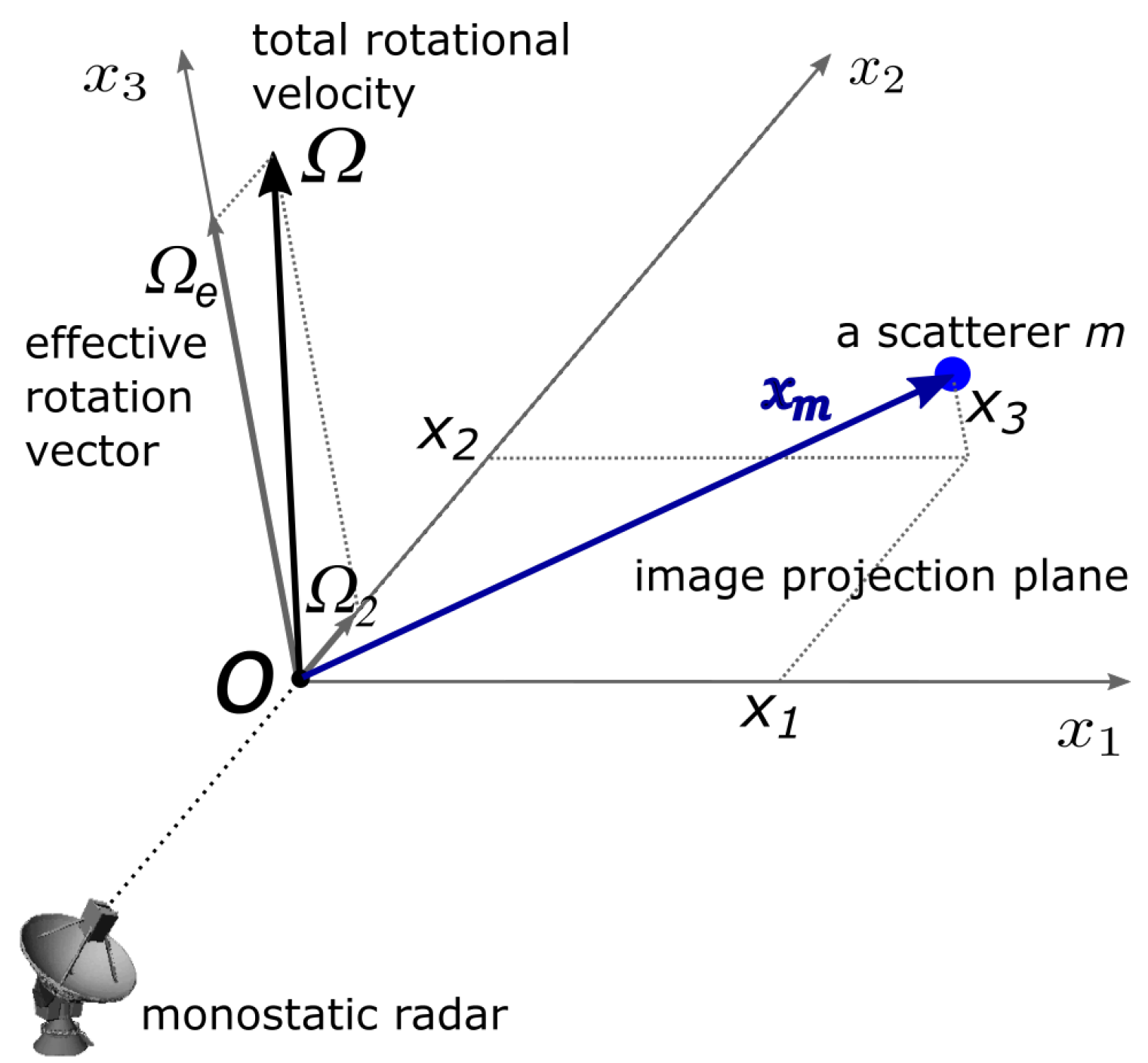
2.1. Signal Model
2.2. Cross-Range Bandwidth and Resolution
2.3. Doppler Radar Tomography (DRT)
2.3.1. The Monostatic DRT Algorithm
- Data segmentation: Partition the N samples of the received signal into L overlapping CPIs of K samples, , ; . These are referred to as ‘segmented CPIs’ below. Denote the overlap factor with . At the midpoint of each segment, the target aspect angle (relative to ) is denoted as ;
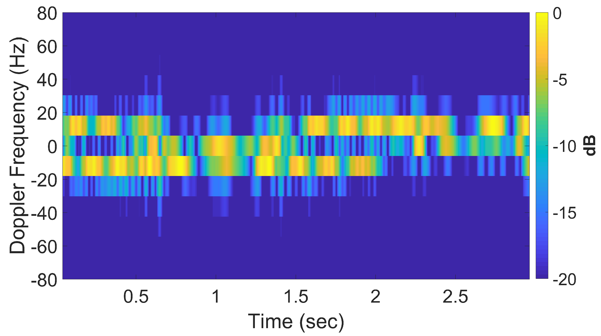
- Translational motion compensation (TMC): this step shifts the Doppler component induced by translational motion to zero Doppler frequency by modulating the segmented CPI by , where is the target’s translational velocity as noted in (5). This quantity is assumed to be known or estimated by other methods. A discrete Fourier transform is then applied to the modulated segments to obtain the Doppler spectrum. The magnitude of the output,is the cross-range (which is proportional to Doppler) profile for the target at an angle from its original orientation. Accumulate all such cross-range profiles for all the corresponding aspect angles , i.e., for all L segmented CPIs.
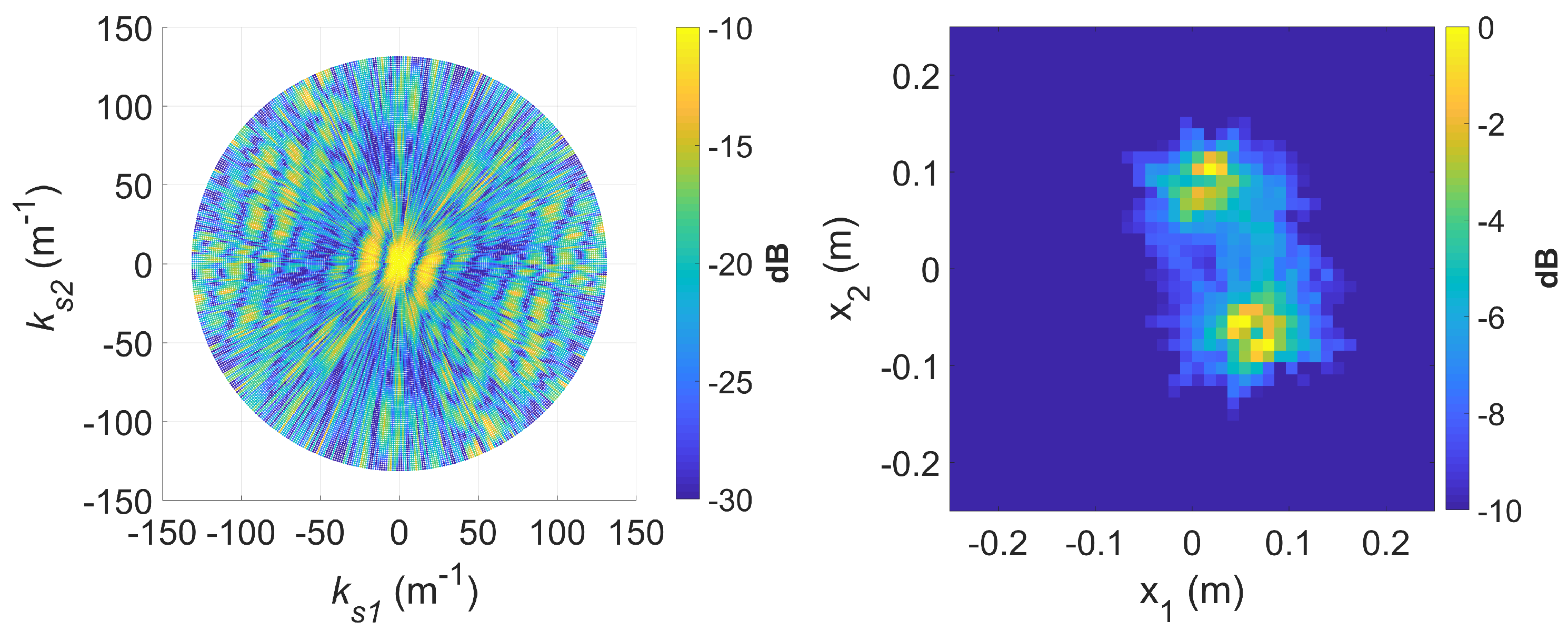
- Populating the k-space: The spatial Fourier transform ofat target aspect angle are then used as the ‘measurement samples’ in the slow-time k-space. As the target rotates, the measurements sweep out a region of support in slow-time k-space as indicated in Figure 2. Due to our choice of reference frames, the measurement population always starts close to the -axis because is the initial cross-range profile.
- Image inversion: An inverse Fourier transform is applied to the populated support of the k-space to yield the target image. Other works have either used filtered back projection, or interpolated the samples onto a rectangular grid to utilise a standard 2D inverse Fourier transform, for this task applied [12,13]. In this paper, we use the non-uniform Fast Fourier transform (NUFFT) [21,22,23,24].
2.3.2. Standard DRT
3. The Slow-Time -Space and Its Augmentation
3.1. The Slow-Time k-Space
3.2. Augmented DRT with Orthogonal Matching Pursuit (OMP)
3.2.1. Sparse Representation
3.2.2. The OMP-Based Augmented DRT Algorithm
- 0.
- Initialize:
- −
- define or select expected intervals of Doppler frequency and chirp rate ;
- −
- define the corresponding chirp atoms and set up the dictionary ;
- −
- input segmented CPI data ;
- 1.
- Compute the OMP-based sparse solution;
- 2.
- Replace all chirp atoms in the sparse solution with single-tone sinusoid functions with Doppler frequency at the mid-point of the segmented CPI;
- 3.
- Compute the focused cross-range profile as given by (24).
- 4.
- Compute NUFFT on the populated slow-time k space to produce the output image.
4. Experimental Results
4.1. Small Target
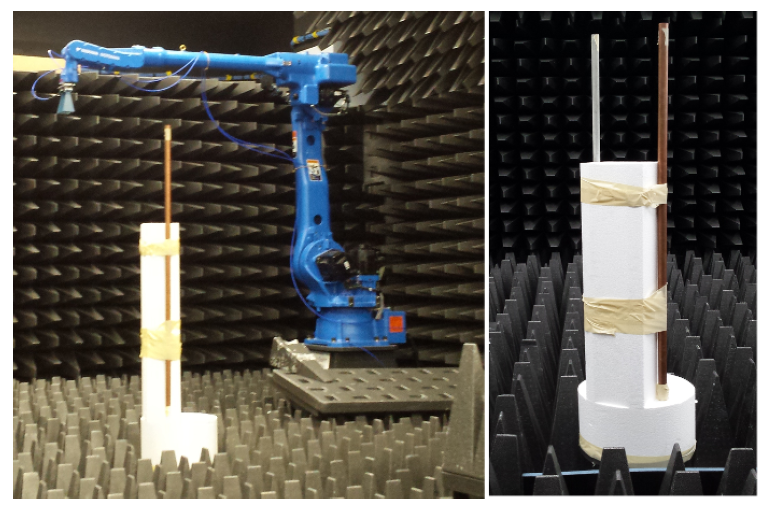
4.1.1. Experimental Setup
4.1.2. System Requirements
- : we choose the lowest and highest frequencies available in this experiment, 8 and 12 GHz, corresponding to or 2.5 cm. With m, or , respectively. We also choose ; the system is thus -limited and poor imaging performance can be expected from standard DRT;
- Inequality (A1) is the Doppler ambiguity free condition; should be designed such that the angular sampling rate (in samp/rad) is greater than (11.7 or 17.6 for this setup), but with as small a margin as possible, to ease hardware requirement.
- The angular sampling interval of per sample in the experiment translates to a samp/rad. Over the chosen value, 100 samples are available. To reduce computational cost while retaining a reasonable FFT length and satisfying the Doppler ambiguity free condition, we use a down sampling ratio of 3:1, leading to samples per CPI, and (samp/rad). This choice also automatically satisfies the constraint in (A8).
4.1.3. Standard DRT Imaging
4.1.4. Augmented DRT Imaging with OMP
4.2. Large Target
4.2.1. Experimental Setup for Large Target
4.2.2. System Requirements
- We choose GHz, corresponding to cm. With m, ; this is well below the typical linear limit of several degrees. The system is thus -limited;
- for this experiment which satisfies inequality (A1) for ambiguity free Doppler frequency.
4.2.3. Standard DRT Imaging
4.2.4. Augmented DRT Imaging with OMP
5. Further Discussion
6. Concluding Remarks
Author Contributions
Funding
Acknowledgments
Conflicts of Interest
Appendix A. Standard DRT: System Parameters and Image Resolution

References
- Kak, A.C.; Slaney, M. Principles of Computerized Tomographic Imaging; Society of Industrial and Applied Mathematics: Philadelphia, PA, USA, 2001. [Google Scholar]
- Tran, H.; Melino, R. The Slow-Time k-Space of Radar Tomography and Applications to High-Resolution Target Imaging. IEEE Trans. Aerosp. Electron. Syst. 2018, 54, 3047–3059. [Google Scholar] [CrossRef]
- Walker, J.L. Range-Doppler Imaging of Rotating Objects. IEEE Trans. Aerosp. Electron. Syst. 1980, AES-16, 23–52. [Google Scholar] [CrossRef]
- Ausherman, D.A.; Kozma, A.; Walker, J.L.; Jones, H.M.; Poggio, E.C. Developments in Radar Imaging. IEEE Trans. Aerosp. Electron. Syst. 1984, AES-20, 363–400. [Google Scholar] [CrossRef]
- Chen, V.C.; Martorella, M. Inverse Synthetic Aperture Radar; Scitech Publishing: Edison, NJ, USA, 2014. [Google Scholar]
- Jakowatz, C.V.; Wahl, D.E.; Eichel, P.H.; Ghiglia, D.C.; Thompson, P. Spotlight-Mode Synthetic Aperture Radar: A Signal Processing Approach; Springer: Berlin/Heidelberg, Germany, 1996. [Google Scholar]
- Soumekh, M. Reconnaissance with slant plane circular SAR imaging. IEEE Trans. Image Process. 1996, 5, 1252–1265. [Google Scholar] [CrossRef] [PubMed]
- Wang, L.; Yazici, B. Bistatic Synthetic Aperture Radar Imaging Using UltraNarrowband Continuous Waveforms. IEEE Trans. Image Process. 2012, 21, 3673–3686. [Google Scholar] [CrossRef] [PubMed]
- Coetzee, S.L.; Baker, C.J.; Griffiths, H.D. Narrow band high resolution radar imaging. In Proceedings of the 2006 IEEE Conference on Radar, Verona, NY, USA, 24–27 April 2006. [Google Scholar]
- Sun, H.; Feng, H.; Lu, Y. High resolution radar tomographic imaging using single-tone CW signals. In Proceedings of the 2010 IEEE Radar Conference, Washington, DC, USA, 10–14 May 2010; pp. 975–980. [Google Scholar]
- Sego, D.J.; Griffiths, H.; Wicks, M.C. Radar tomography using Doppler-based projections. In Proceedings of the 2011 IEEE RadarCon (RADAR), Kansas City, MO, USA, 23–27 May 2011; pp. 403–408. [Google Scholar]
- Mensa, D.L.; Halevy, S.; Wade, G. Coherent Doppler tomography for microwave imaging. Proc. IEEE 1983, 71, 254–261. [Google Scholar] [CrossRef]
- Tran, H.T.; Melino, R. Application of the Fractional Fourier Transform and S-Method in Doppler Radar Tomography; Technical Report DSTO-RR-0357; The Defence Science and Technology Organisation: Edinburgh, Australia, 2010. [Google Scholar]
- Chen, V.; Ling, H. Time-Frequency Transforms for Radar Imaging and Signal Analysis; Artech House: Norwood, MA, USA, 2003. [Google Scholar]
- Potter, L.C.; Ertin, E.; Parker, J.T.; Cetin, M. Sparsity and Compressed Sensing in Radar Imaging. Proc. IEEE 2010, 98, 1006–1020. [Google Scholar] [CrossRef]
- Kodituwakku, S.; Melino, R.; Berry, P.; Tran, H. Tilted-wire scatterer model for narrowband radar imaging of rotating blades. IET Radar Sonar Navig. 2017, 11, 640–645. [Google Scholar] [CrossRef]
- Melino, R.; Kodituwakku, S.; Tran, H. Orthogonal matching pursuit and matched filter techniques for the imaging of rotating blades. In Proceedings of the 2015 IEEE Radar Conference, Johannesburg, South Africa, 27–30 October 2015; pp. 1–6. [Google Scholar]
- Tran, H.; Heading, E.; Melino, R. OMP-based translational motion estimation for a rotating target by narrowband radar. IET Radar Sonar Navig. 2017, 11, 854–860. [Google Scholar] [CrossRef]
- Baker, C.J.; Griffiths, H.D. Bistatic and Multistatic Radar Sensors for Homeland Security. In Advances in Sensing with Security Applications; Springer: Dordrecht, The Netherlands, 2006; pp. 1–22. [Google Scholar]
- Cilliers, A.; Nel, W.A.J. Helicopter parameter extraction using joint time-frequency and tomographic techniques. In Proceedings of the 2008 International Conference on Radar, Adelaide, SA, Australia, 2–5 September 2008; pp. 598–603. [Google Scholar]
- Dutt, A.; Rokhlin, V. Fast Fourier Transforms for Nonequispaced Data, II. Appl. Comput. Harmon. Anal. 1995, 2, 85–100. [Google Scholar] [CrossRef]
- Nguyen, N.; Liu, Q.H. The Regular Fourier Matrices and Nonuniform Fast Fourier Transform. SIAM J. Sci. Comput. 1999, 21, 283–293. [Google Scholar] [CrossRef]
- Greengard, L.; Lee, J. Accelerating the Nonuniform Fast Fourier Transform. SIAM Rev. 2004, 46, 443–454. [Google Scholar] [CrossRef]
- Ferrara, M. AFOSR Lab Task ‘Moving-Target Radar Feature Extraction’. 2009. Available online: https://au.mathworks.com/matlabcentral/fileexchange/25135-nufft--nfft--usfft/all_files (accessed on 7 November 2010).
- Tran, H.; Heading, E.; Ng, B. Multi-Bistatic Doppler Radar Tomography for Non-Cooperative Target Imaging. In Proceedings of the 2018 International Conference on Radar (RADAR), Brisbane, Australia, 27–30 August 2018; pp. 1–6. [Google Scholar]
- Elad, M. Sparse and Redundant Representations: From Theory to Applications in Signal and Image Processing; Springer: Berlin/Heidelberg, Germany, 2010. [Google Scholar]
- Fliss, F. Tomographic Radar Imaging of Rotating Structures. In Synthetic Aperture Radar; International Society for Optics and Photonics: Los Angeles, CA, USA, 1992; Volume 1630. [Google Scholar]
- Munson, D.C.; O’Brien, J.D.; Jenkins, W.K. A tomographic formulation of spotlight-mode synthetic aperture radar. Proc. IEEE 1983, 71, 917–925. [Google Scholar] [CrossRef]
- Knott, E.F.; Shaeffer, J.F.; Tuley, M.T. Radar Cross Section, 2nd ed.; SciTech Publishing Inc: Rayleigh, NC, USA, 2004. [Google Scholar]
- Nguyen, N.H.; Dogancay, K.; Tran, H.; Berry, P.E. Parameter-Refined OMP for Compressive Radar Imaging of Rotating Targets. IEEE Trans. Aerosp. Electron. Syst. 2019, 55, 3561–3577. [Google Scholar] [CrossRef]


| Cylinder | (m) | Diameter (m) | Height (m) |
|---|---|---|---|
| 1 | 2.5 | 0.15 | 0.30 |
| 2 | 5 | 0.38 | 0.18 |
| 3 | 8 | 0.21 | 0.46 |
© 2020 Commonwealth of Australia. Licensee MDPI, Basel, Switzerland. This article is an open access article distributed under the terms and conditions of the Creative Commons Attribution (CC BY) license (http://creativecommons.org/licenses/by/4.0/).
Share and Cite
Tran, H.-T.; Heading, E.; Ng, B.W.-H. On the Slow-Time k-Space and its Augmentation in Doppler Radar Tomography. Sensors 2020, 20, 513. https://doi.org/10.3390/s20020513
Tran H-T, Heading E, Ng BW-H. On the Slow-Time k-Space and its Augmentation in Doppler Radar Tomography. Sensors. 2020; 20(2):513. https://doi.org/10.3390/s20020513
Chicago/Turabian StyleTran, Hai-Tan, Emma Heading, and Brian W.-H. Ng. 2020. "On the Slow-Time k-Space and its Augmentation in Doppler Radar Tomography" Sensors 20, no. 2: 513. https://doi.org/10.3390/s20020513
APA StyleTran, H.-T., Heading, E., & Ng, B. W.-H. (2020). On the Slow-Time k-Space and its Augmentation in Doppler Radar Tomography. Sensors, 20(2), 513. https://doi.org/10.3390/s20020513