Application of UAV in Topographic Modelling and Structural Geological Mapping of Quarries and Their Surroundings—Delineation of Fault-Bordered Raw Material Reserves


Abstract

1. Introduction
2. Study Area
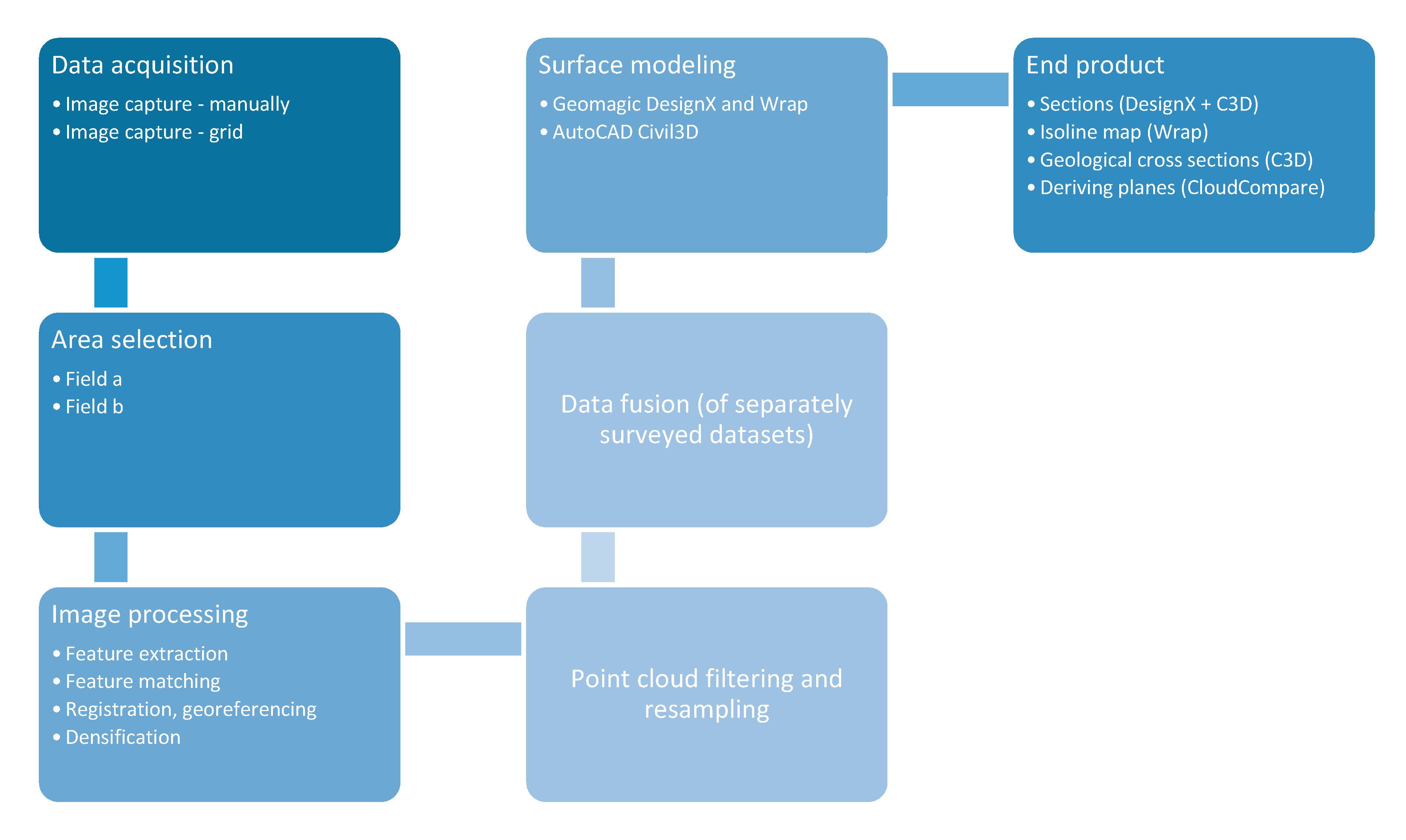
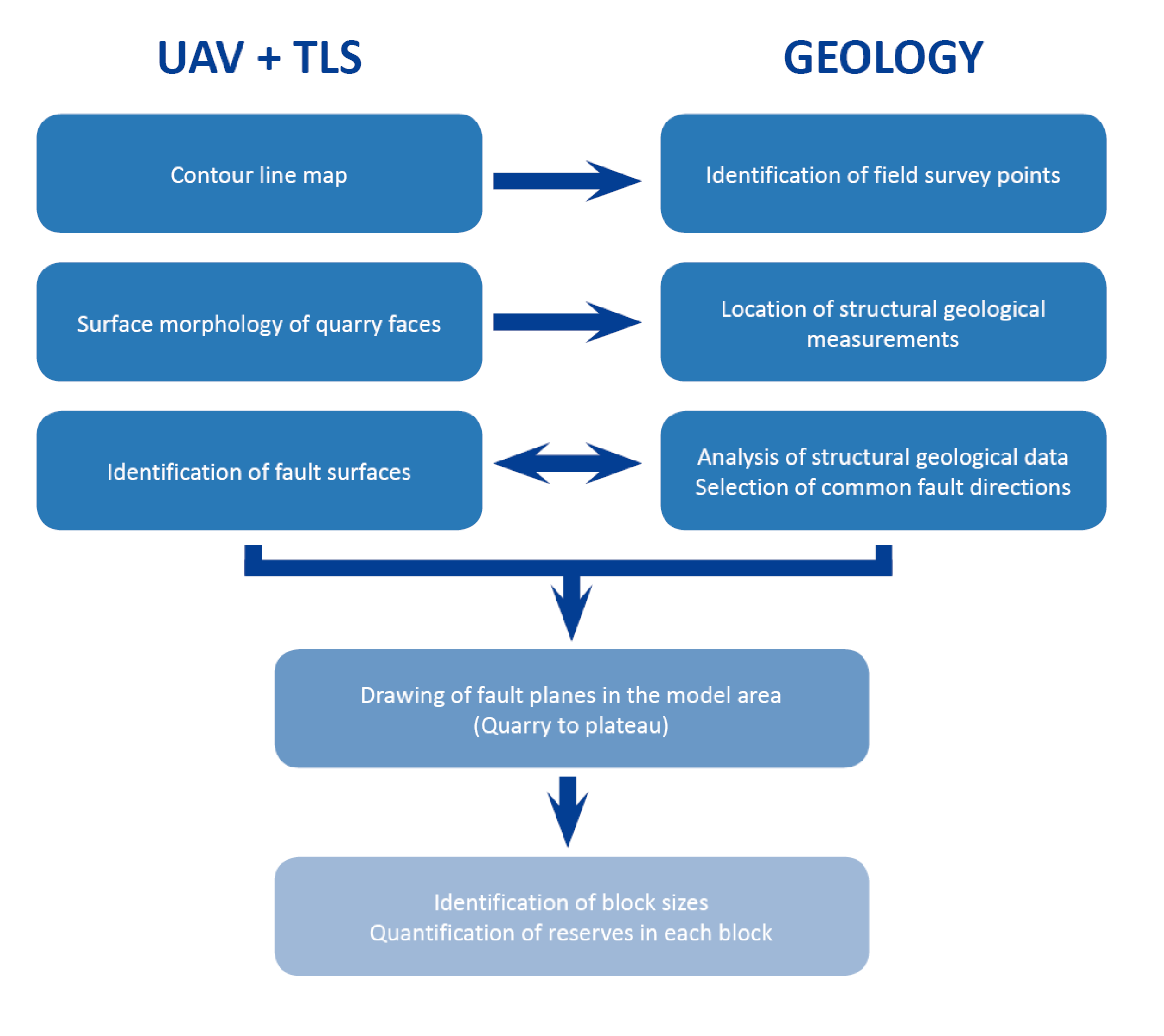
3. Methods
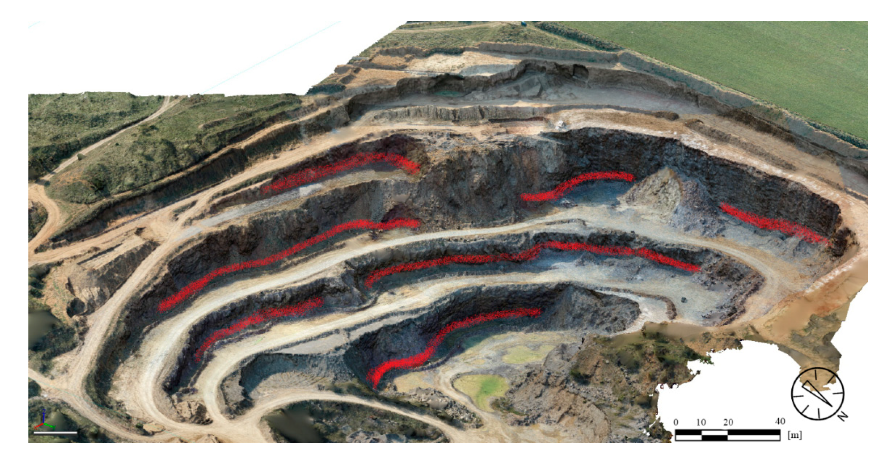
4. Results
5. Discussion
6. Conclusions
Author Contributions
Funding
Acknowledgments
Conflicts of Interest
References
- Chen, J.; Dowman, I.; Li, S.; Li, Z.; Madden, M.; Mills, J.; Paparoditis, N.; Rottensteiner, F.; Sester, M.; Toth, C.; et al. Information from imagery: ISPRS scientific vision and research agenda. ISPRS J. Photogramm. Remote Sens. 2016, 115, 3–21. [Google Scholar] [CrossRef]
- Scholtz, A.; Kaschwich, C.; Krüger, A.; Kufieta, K.; Schnetter, P.; Wilkens, C.-S.; Krüger, T.; Vörsmann, P. Developement of a new multi-purpose UAS for scientific application. ISPRS Int. Arch. Photogramm. Remote Sens. Spat. Inf. Sci. 2012, XXXVIII-1/C22, 149–154. [Google Scholar] [CrossRef]
- Colomina, I.; Molina, P. Unmanned aerial systems for photogrammetry and remote sensing: A review. ISPRS J. Photogramm. Remote Sens. 2014, 92, 79–97. [Google Scholar] [CrossRef]
- Fritz, A.; Kattenborn, T.; Koch, B. UAV-based photogrammetric point clouds-tree stem mapping in open stands in comparison to terrestrial laser scanner point clouds. ISPRS Int. Arch. Photogramm. Remote Sens. Spat. Inf. Sci. 2013, XL-1/W2, 141–146. [Google Scholar] [CrossRef]
- Campana, S. Drones in Archaeology. State-of-the-art and Future Perspectives: Drones in Archaeology. Archaeol. Prospect. 2017, 24, 275–296. [Google Scholar] [CrossRef]
- Margottini, C.; Antidze, N.; Corominas, J.; Crosta, G.B.; Frattini, P.; Gigli, G.; Giordan, D.; Iwasaky, I.; Lollino, G.; Manconi, A.; et al. Landslide hazard, monitoring and conservation strategy for the safeguard of Vardzia Byzantine monastery complex, Georgia. Landslides 2015, 12, 193–204. [Google Scholar] [CrossRef][Green Version]
- Boccardo, P.; Chiabrando, F.; Dutto, F.; Tonolo, F.; Lingua, A. UAV Deployment Exercise for Mapping Purposes: Evaluation of Emergency Response Applications. Sensors 2015, 15, 15717–15737. [Google Scholar] [CrossRef]
- Wierzbicki, D. Multi-Camera Imaging System for UAV Photogrammetry. Sensors 2018, 18, 2433. [Google Scholar] [CrossRef]
- Agüera-Vega, F.; Carvajal-Ramírez, F.; Martínez-Carricondo, P.; Sánchez-Hermosilla López, J.; Mesas-Carrascosa, F.J.; García-Ferrer, A.; Pérez-Porras, F.J. Reconstruction of extreme topography from UAV structure from motion photogrammetry. Measurement 2018, 121, 127–138. [Google Scholar] [CrossRef]
- Cappelletti, C.; Boniardi, M.; Casaroli, A.; De Gaetani, C.I.; Passoni, D.; Pinto, L. Forensic engineering surverys with UAV photogrammetry and laser scanning techniques. ISPRS Int. Arch. Photogramm. Remote Sens. Spat. Inf. Sci. 2019, XLII-2/W9, 227–234. [Google Scholar] [CrossRef]
- He, H.; Chen, T.; Zeng, H.; Huang, S. Ground Control Point-Free Unmanned Aerial Vehicle-Based Photogrammetry for Volume Estimation of Stockpiles Carried on Barges. Sensors 2019, 19, 3534. [Google Scholar] [CrossRef] [PubMed]
- Escobar Villanueva, J.R.; Iglesias Martínez, L.; Pérez Montiel, J.I. DEM Generation from Fixed-Wing UAV Imaging and LiDAR-Derived Ground Control Points for Flood Estimations. Sensors 2019, 19, 3205. [Google Scholar] [CrossRef] [PubMed]
- Niedzielski, T.; Witek, M.; Spallek, W. Observing river stages using unmanned aerial vehicles. Hydrol. Earth Syst. Sci. 2016, 20, 3193–3205. [Google Scholar] [CrossRef]
- Langhammer, J.; Lendzioch, T.; Miřijovský, J.; Hartvich, F. UAV-Based Optical Granulometry as Tool for Detecting Changes in Structure of Flood Depositions. Remote Sens. 2017, 9, 240. [Google Scholar] [CrossRef]
- Neugirg, F.; Stark, M.; Kaiser, A.; Vlacilova, M.; Della Seta, M.; Vergari, F.; Schmidt, J.; Becht, M.; Haas, F. Erosion processes in calanchi in the Upper Orcia Valley, Southern Tuscany, Italy based on multitemporal high-resolution terrestrial LiDAR and UAV surveys. Geomorphology 2016, 269, 8–22. [Google Scholar] [CrossRef]
- Langhammer, J. UAV Monitoring of Stream Restorations. Hydrology 2019, 6, 29. [Google Scholar] [CrossRef]
- Ong, W.; Chiu, W.; Kuen, T.; Kodikara, J. Determination of the State of Strain of Large Floating Covers Using Unmanned Aerial Vehicle (UAV) Aided Photogrammetry. Sensors 2017, 17, 1731. [Google Scholar] [CrossRef]
- Shahbazi, M.; Sohn, G.; Théau, J.; Menard, P. Development and Evaluation of a UAV-Photogrammetry System for Precise 3D Environmental Modeling. Sensors 2015, 15, 27493–27524. [Google Scholar] [CrossRef]
- Nex, F.; Rupnik, E.; Toschi, I.; Remondino, F. Automated processing of high resolution airborne images for earthquake damage assessment. ISPRS Int. Arch. Photogramm. Remote Sens. Spat. Inf. Sci. 2014, XL–1, 315–321. [Google Scholar] [CrossRef]
- Achille, C.; Adami, A.; Chiarini, S.; Cremonesi, S.; Fassi, F.; Fregonese, L.; Taffurelli, L. UAV-Based Photogrammetry and Integrated Technologies for Architectural Applications—Methodological Strategies for the After-Quake Survey of Vertical Structures in Mantua (Italy). Sensors 2015, 15, 15520–15539. [Google Scholar] [CrossRef]
- Comba, L.; Biglia, A.; Ricauda Aimonino, D.; Gay, P. Unsupervised detection of vineyards by 3D point-cloud UAV photogrammetry for precision agriculture. Comput. Electron. Agric. 2018, 155, 84–95. [Google Scholar] [CrossRef]
- Dering, G.M.; Micklethwaite, S.; Thiele, S.T.; Vollgger, S.A.; Cruden, A.R. Review of drones, photogrammetry and emerging sensor technology for the study of dykes: Best practises and future potential. J. Volcanol. Geotherm. Res. 2019, 373, 148–166. [Google Scholar] [CrossRef]
- Giordan, D.; Allasia, P.; Dematteis, N.; Dell’Anese, F.; Vagliasindi, M.; Motta, E. A Low-Cost Optical Remote Sensing Application for Glacier Deformation Monitoring in an Alpine Environment. Sensors 2016, 16, 1750. [Google Scholar] [CrossRef] [PubMed]
- Chudley, T.R.; Christoffersen, P.; Doyle, S.H.; Abellan, A.; Snooke, N. High accuracy UAV photogrammetry of ice sheet dynamics with no ground control. Cryosphere Discuss. 2018, 1–22. [Google Scholar] [CrossRef]
- Rossini, M.; Di Mauro, B.; Garzonio, R.; Baccolo, G.; Cavallini, G.; Mattavelli, M.; De Amicis, M.; Colombo, R. Rapid melting dynamics of an alpine glacier with repeated UAV photogrammetry. Geomorphology 2018, 304, 159–172. [Google Scholar] [CrossRef]
- Miziński, B.; Niedzielski, T. Fully-automated estimation of snow depth in near real time with the use of unmanned aerial vehicles without utilizing ground control points. Cold Reg. Sci. Technol. 2017, 138, 63–72. [Google Scholar] [CrossRef]
- Niedzielski, T.; Szymanowski, M.; Miziński, B.; Spallek, W.; Witek-Kasprzak, M.; Ślopek, J.; Kasprzak, M.; Błaś, M.; Sobik, M.; Jancewicz, K.; et al. Estimating snow water equivalent using unmanned aerial vehicles for determining snow-melt runoff. J. Hydrol. 2019, 578, 124046. [Google Scholar] [CrossRef]
- Zekkos, D.; Greenwood, W.; Lynch, J.; Manousakis, J.; Athanasopoulos-Zekkos, A.; Clark, M.; Saroglou, C. Lessons Learned from The Application of UAV-Enabled Structure-From-Motion Photogrammetry in Geotechnical Engineering. Int. J. Geoeng. Case Hist. 2018, 4, 254–274. [Google Scholar] [CrossRef]
- Török, Á.; Barsi, Á.; Bögöly, G.; Lovas, T.; Somogyi, Á.; Görög, P. Slope stability and rockfall assessment of volcanic tuffs using RPAS with 2-D FEM slope modelling. Nat. Hazards Earth Syst. Sci. 2018, 18, 583–597. [Google Scholar] [CrossRef]
- Tannant, D. Review of Photogrammetry-Based Techniques for Characterization and Hazard Assessment of Rock Faces. Int. J. Geohazards Environ. 2015, 76–87. [Google Scholar] [CrossRef]
- Tannant, D.D.; Giordan, D.; Morgenroth, J. Characterization and analysis of a translational rockslide on a stepped-planar slip surface. Eng. Geol. 2017, 220, 144–151. [Google Scholar] [CrossRef]
- Francioni, M.; Salvini, R.; Stead, D.; Litrico, S. A case study integrating remote sensing and distinct element analysis to quarry slope stability assessment in the Monte Altissimo area, Italy. Eng. Geol. 2014, 183, 290–302. [Google Scholar] [CrossRef]
- Bartolo, S.D.; Salvini, R. Multitemporal Terrestrial Laser Scanning for Marble Extraction Assessment in an Underground Quarry of the Apuan Alps (Italy). Sensors 2019, 19, 450. [Google Scholar] [CrossRef] [PubMed]
- Giordan, D.; Hayakawa, Y.; Nex, F.; Remondino, F.; Tarolli, P. Review article: The use of remotely piloted aircraft systems (RPASs) for natural hazards monitoring and management. Nat. Hazards Earth Syst. Sci. 2018, 18, 1079–1096. [Google Scholar] [CrossRef]
- Mancini, F.; Dubbini, M.; Gattelli, M.; Stecchi, F.; Fabbri, S.; Gabbianelli, G. Using Unmanned Aerial Vehicles (UAV) for High-Resolution Reconstruction of Topography: The Structure from Motion Approach on Coastal Environments. Remote Sens. 2013, 5, 6880–6898. [Google Scholar] [CrossRef]
- Saroglou, C.; Kallimogiannis, V.; Bar, N.; Manousakis, G.; Zekkos, D. Analysis of slope instabilities in the Corinth Canal using UAV-enabled mapping. In Proceedings of the ICONHIC 2nd International Conference on Natural Hazards & Infrastructure, Chania, Greece, 23–26 June 2019. [Google Scholar]
- Salvini, R.; Mastrorocco, G.; Seddaiu, M.; Rossi, D.; Vanneschi, C. The use of an unmanned aerial vehicle for fracture mapping within a marble quarry (Carrara, Italy): Photogrammetry and discrete fracture network modelling. Geomat. Nat. Hazards Risk 2017, 8, 34–52. [Google Scholar] [CrossRef]
- Martin, P.G.; Payton, O.D.; Fardoulis, J.S.; Richards, D.A.; Scott, T.B. The use of unmanned aerial systems for the mapping of legacy uranium mines. J. Environ. Radioact. 2015, 143, 135–140. [Google Scholar] [CrossRef]
- Török, Á. Controls on development of Mid-Triassic ramps: Examples from southern Hungary. Geol. Soc. Lond. Spec. Publ. 1998, 149, 339–367. [Google Scholar] [CrossRef]
- Götz, A.E.; Török, Á. Correlation of Tethyan and Peri-Tethyan long-term and high-frequency eustatic signals (Anisian, Middle Triassic). Geol. Carpathica 2008, 59, 307–317. [Google Scholar]
- Götz, A.E.; Török, Á. Muschelkalk Ramp Cycles Revisited. In Stratigraphy & Timescales; Elsevier: Amsterdam, The Netherlands, 2018; Volume 3, pp. 265–284. ISBN 978-0-12-815098-6. [Google Scholar] [CrossRef]
- Gao, M.; Xu, X.; Klinger, Y.; van der Woerd, J.; Tapponnier, P. High-resolution mapping based on an Unmanned Aerial Vehicle (UAV) to capture paleoseismic offsets along the Altyn-Tagh fault, China. Sci. Rep. 2017, 7, 8281. [Google Scholar] [CrossRef]
- Menegoni, N.; Meisina, C.; Perotti, C.; Crozi, M. Analysis by UAV Digital Photogrammetry of Folds and Related Fractures in the Monte Antola Flysch Formation (Ponte Organasco, Italy). Geosciences 2018, 8, 299. [Google Scholar] [CrossRef]
- Sayab, M.; Aerden, D.; Paananen, M.; Saarela, P. Virtual Structural Analysis of Jokisivu Open Pit Using ‘Structure-from-Motion’ Unmanned Aerial Vehicles (UAV) Photogrammetry: Implications for Structurally-Controlled Gold Deposits in Southwest Finland. Remote Sens. 2018, 10, 1296. [Google Scholar] [CrossRef]
- Haas, F.; Hilger, L.; Neugirg, F.; Umstädter, K.; Breitung, C.; Fischer, P.; Hilger, P.; Heckmann, T.; Dusik, J.; Kaiser, A.; et al. Quantification and analysis of geomorphic processes on a recultivated iron ore mine on the Italian island of Elba using long-term ground-based lidar and photogrammetric SfM data by a UAV. Nat. Hazards Earth Syst. Sci. 2016, 16, 1269–1288. [Google Scholar] [CrossRef]
- Vanneschi, C.; Di Camillo, M.; Aiello, E.; Bonciani, F.; Salvini, R. SfM-MVS Photogrammetry for Rockfall Analysis and Hazard Assessment Along the Ancient Roman Via Flaminia Road at the Furlo Gorge (Italy). ISPRS Int. J. Geo-Inf. 2019, 8, 325. [Google Scholar] [CrossRef]
- Pappalardo, G.; Mineo, S.; Rapisarda, F. Rockfall hazard assessment along a road on the Peloritani Mountains (northeastern Sicily, Italy). Nat. Hazards Earth Syst. Sci. 2014, 14, 2735–2748. [Google Scholar] [CrossRef]
- Mazzanti, P.; Schilirò, L.; Martino, S.; Antonielli, B.; Brizi, E.; Brunetti, A.; Margottini, C.; Scarascia Mugnozza, G. The Contribution of Terrestrial Laser Scanning to the Analysis of Cliff Slope Stability in Sugano (Central Italy). Remote Sens. 2018, 10, 1475. [Google Scholar] [CrossRef]
- Geological Map Hungary, Scale 1:100000. Magyarország 1:100,000 Méretarányú Fedett Földtani Térképe; Geological Institute of Hungary: Budapest, Hungary, 2005. Available online: https://map.mbfsz.gov.hu/ (accessed on 14 January 2020). (In Hungarian)
- DJI. Available online: https://www.dji.com/hu/phantom-4-pro (accessed on 30 September 2019).
- Flylitchi. Available online: https://flylitchi.com/ (accessed on 30 September 2019).
- Cawood, A.J.; Bond, C.E.; Howell, J.A.; Butler, R.W.H.; Totake, Y. LiDAR, UAV or compass-clinometer? Accuracy, coverage and the effects on structural models. J. Struct. Geol. 2017, 98, 67–82. [Google Scholar] [CrossRef]
- Jordá Bordehore, L.; Riquelme, A.; Cano, M.; Tomás, R. Comparing manual and remote sensing field discontinuity collection used in kinematic stability assessment of failed rock slopes. Int. J. Rock Mech. Min. Sci. 2017, 97, 24–32. [Google Scholar] [CrossRef]


| - | Faro Focus 120 Parameters |
|---|---|
| ranging technique | phase-based |
| ranging accuracy | +/− 2 mm |
| applied point spacing | 6 mm @ 10 m |
| number of scan positions | 98 |
| number of scanned points | 588 M |
| quarry area covered | 0.15 km2 |
| - | X [mm] | Y [mm] | Z [mm] |
|---|---|---|---|
| GCP 1 | –0.5 | –20.1 | 0.1 |
| GCP 2 | 8.0 | –19.5 | 22.1 |
| GCP 3 | –22.6 | –19.5 | 28.7 |
| GCP 4 | –22.5 | 18.8 | –13.1 |
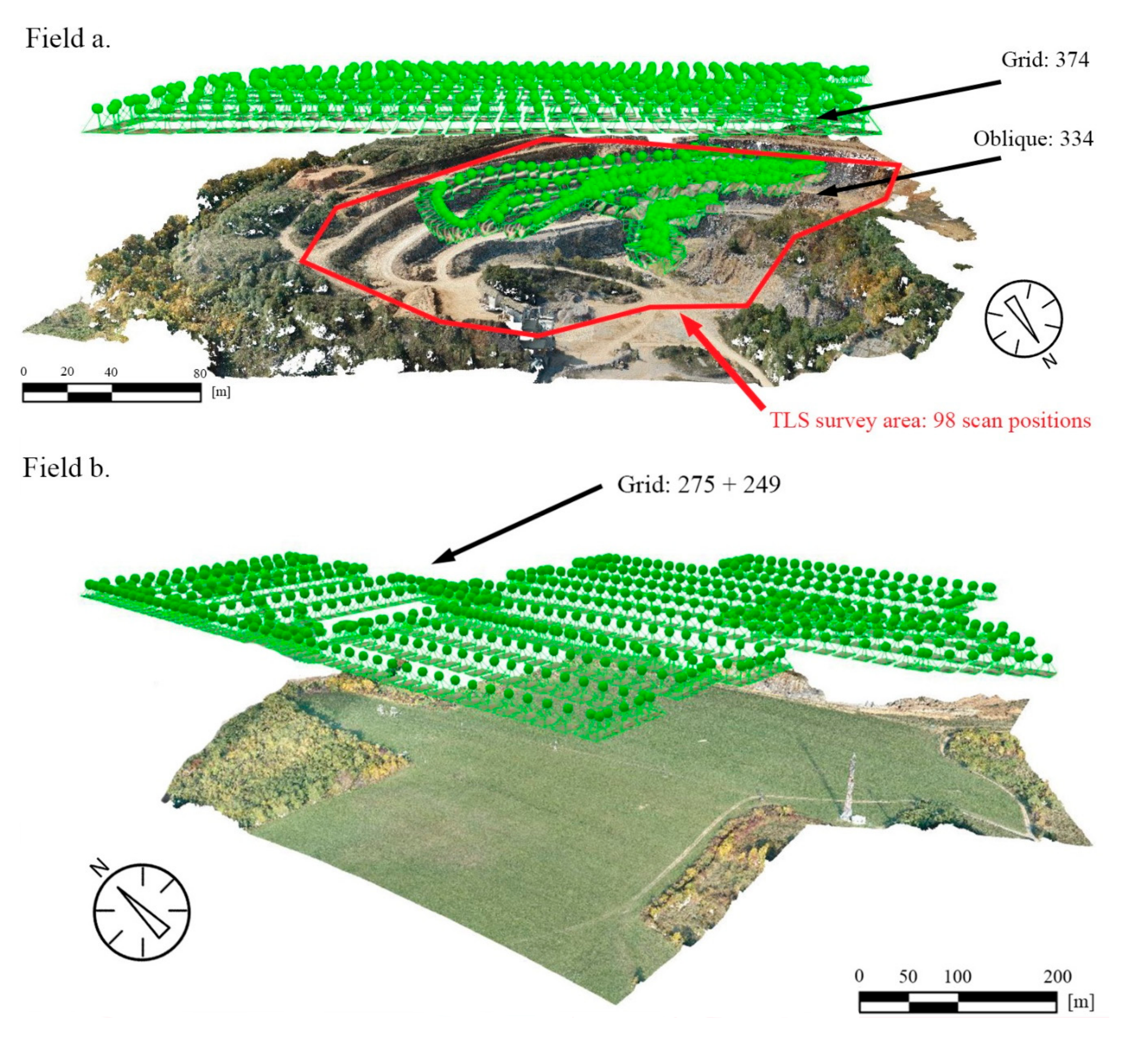
| - | Field a (Quarry Area) | Field b (Plateau Area) | ||
|---|---|---|---|---|
| Sensor Parameters | focal length: 8.8 mm, sensor size: 12.833 × 8.556 mm | |||
| Image Size | 5472 × 3648 (RGB) | |||
| Flight | I | II | III | IV |
| Flight Mode | Oblique | Grid | Grid | Grid |
| Height | Various | 140.5 | 120.9 m | 120.9 m |
| Length | - | 5.1 km | 4.4 km | 3.3 km |
| Image Count | 334 | 374 | 275 | 249 |
| Overlap between Images | various | >75% (between rows), >80% (between consecutive images) | ||
| Area Covered | 0.256 km2 | 0.654 km2 | ||
| Average GSD | 2.57 cm | 3.15 cm | ||
| Used GCP | 14 | 14 | ||
| GCP’s RMS (x,y,z) | 2.0, 1.9, 2.7 cm | 1.2, 1.1, 7.0 cm | ||
| Mean Number of 2D Keypoint | 23,058 | 29,480 | ||
| Mean Number of 3D Tiepoint | 6,462 | 7,557 | ||
| Mean Reprojection Error | 0.12 pixel | 0.13 pixel | ||
| Image Scale for Densification | 1/1 | ½ | ||
| Number of 3D Densified Points | 320,727,823 | 58,551,776 | ||
| Average Density | 970.47 | 129.22 | ||
© 2020 by the authors. Licensee MDPI, Basel, Switzerland. This article is an open access article distributed under the terms and conditions of the Creative Commons Attribution (CC BY) license (http://creativecommons.org/licenses/by/4.0/).
Share and Cite
Török, Á.; Bögöly, G.; Somogyi, Á.; Lovas, T. Application of UAV in Topographic Modelling and Structural Geological Mapping of Quarries and Their Surroundings—Delineation of Fault-Bordered Raw Material Reserves. Sensors 2020, 20, 489. https://doi.org/10.3390/s20020489
Török Á, Bögöly G, Somogyi Á, Lovas T. Application of UAV in Topographic Modelling and Structural Geological Mapping of Quarries and Their Surroundings—Delineation of Fault-Bordered Raw Material Reserves. Sensors. 2020; 20(2):489. https://doi.org/10.3390/s20020489
Chicago/Turabian StyleTörök, Ákos, Gyula Bögöly, Árpád Somogyi, and Tamás Lovas. 2020. "Application of UAV in Topographic Modelling and Structural Geological Mapping of Quarries and Their Surroundings—Delineation of Fault-Bordered Raw Material Reserves" Sensors 20, no. 2: 489. https://doi.org/10.3390/s20020489
APA StyleTörök, Á., Bögöly, G., Somogyi, Á., & Lovas, T. (2020). Application of UAV in Topographic Modelling and Structural Geological Mapping of Quarries and Their Surroundings—Delineation of Fault-Bordered Raw Material Reserves. Sensors, 20(2), 489. https://doi.org/10.3390/s20020489