Evaluation of Recent Advanced Soft Computing Techniques for Gully Erosion Susceptibility Mapping: A Comparative Study

 ,
,  ,
,  ,
,  ,
,  and
and
Abstract
1. Introduction
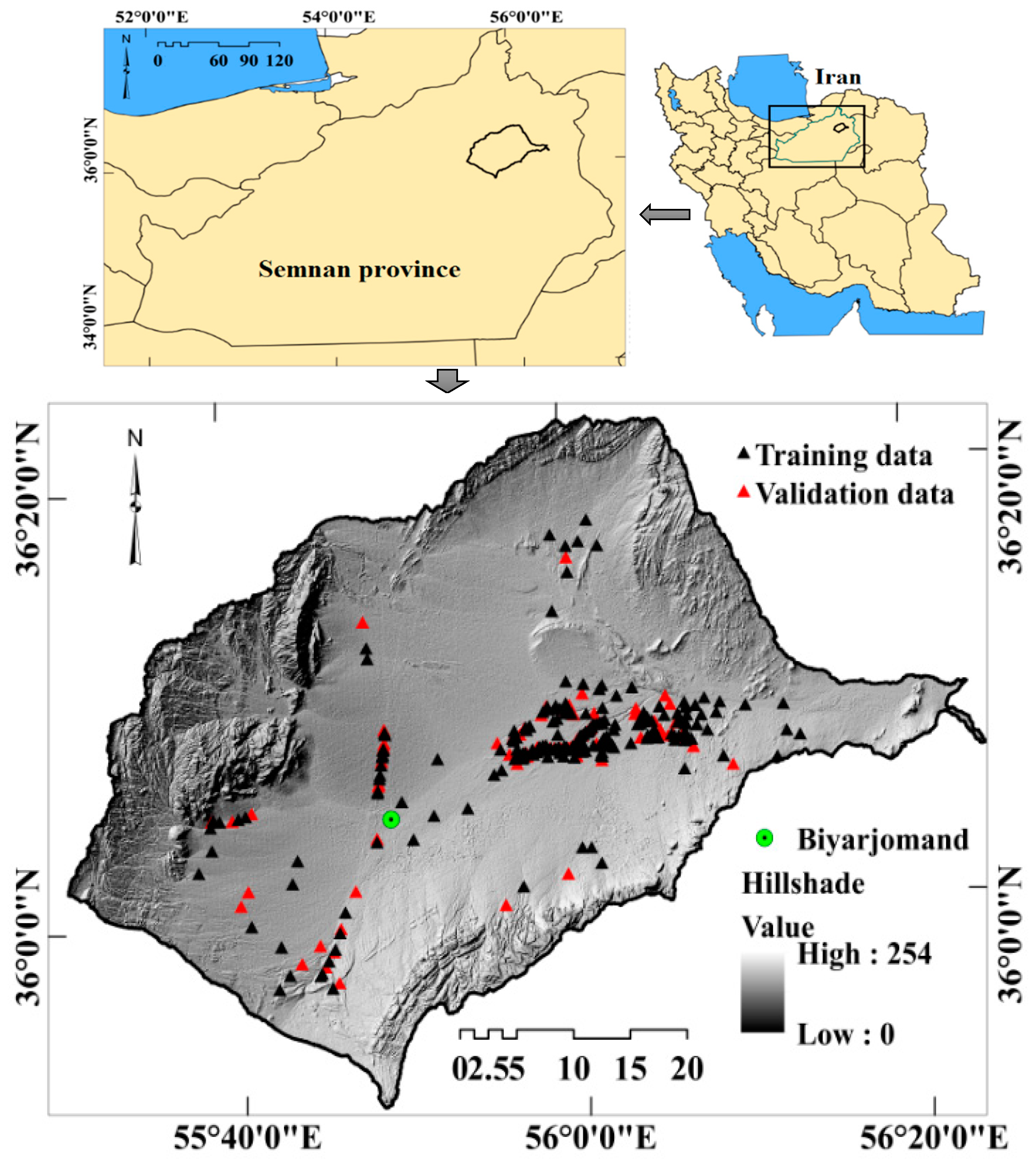
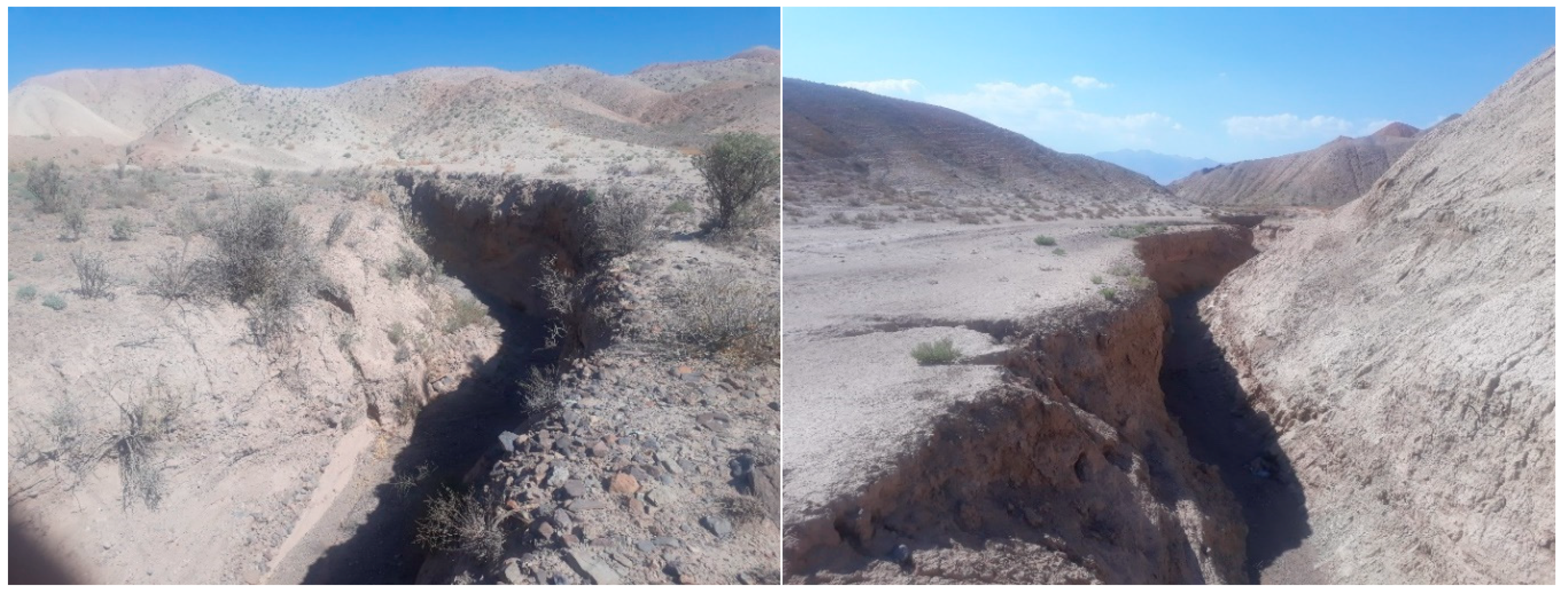
2. Description of the Study Area
3. Materials and Methods
3.1. Data Used
3.2. Background of the Methods Used
3.2.1. Frequency Ratio (FR) and Statistical Index (SI)
3.2.2. Random Forest (RF)
3.2.3. Maximum Entropy (ME)
3.2.4. Generalized Linear Model (GLM)
3.2.5. Functional Data Analysis (FDA)
3.2.6. Technique for Order Preference by Similarity to Ideal Solution (TOPSIS)
3.2.7. Ensemble Approaches (GLM–FDA, FR–RF and SI–RF)
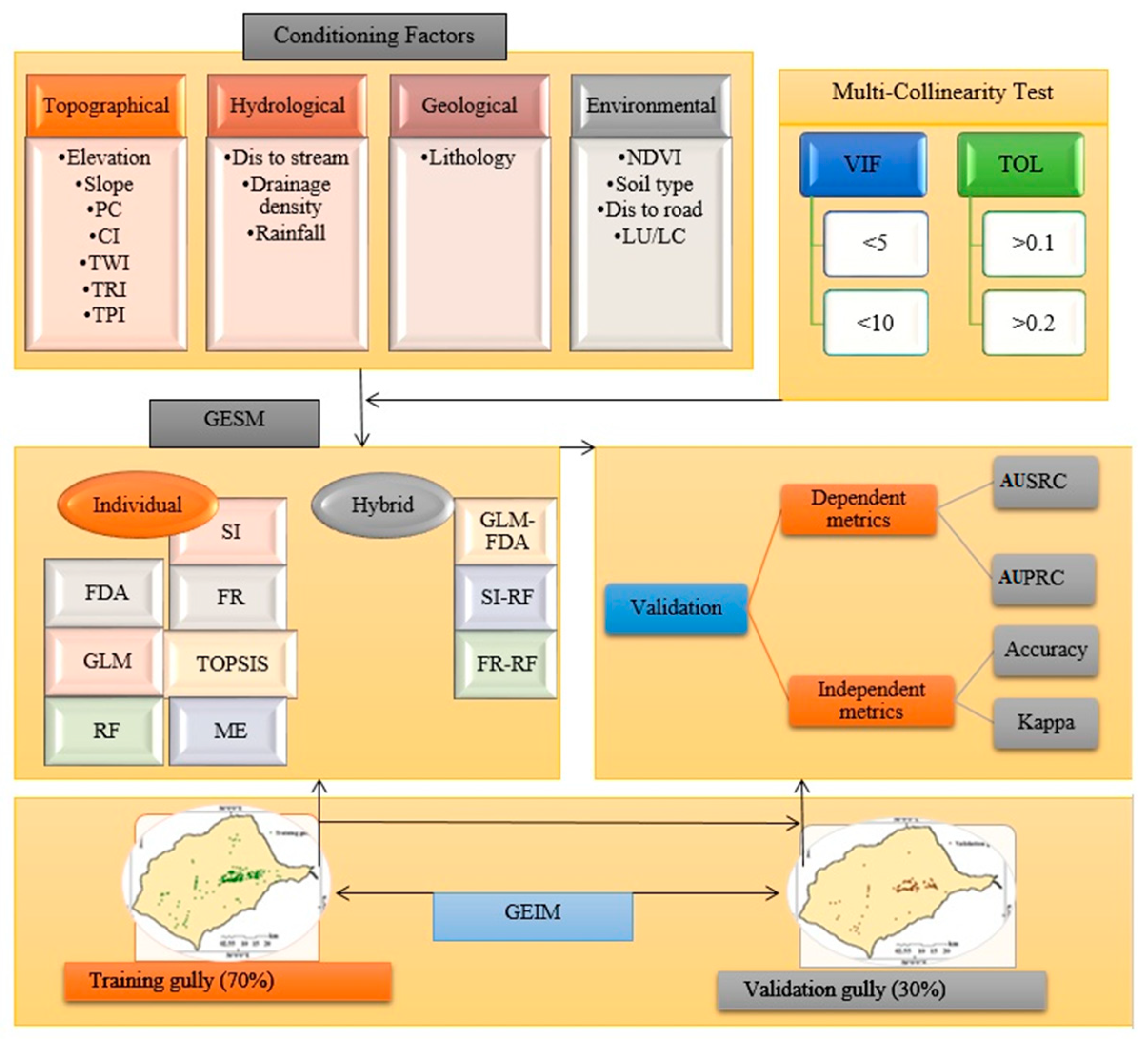
3.3. Methodology
- Step 1:
- Database preparation.
- Step 2:
- Multicollinearity analysis. If collinearity occurs among the parameters, the prediction accuracy of a model will decrease [3]. Indices of tolerance (TOL) and variance inflation factor (VIF) were used to evaluate collinearity [70]. If VIF ≤ 5 or 10 and TOL≤ 0.1 or 0.2, then no collinearity exists between factors [71].
- Step 3:
- Configuring and training the GE models.
- Step 4:
- Performance assessment using cutoff dependence (Area under prediction rate curve [AUPRC] and area under success rate curve [AUSRC]) and cutoff independence (accuracy and kappa).
- Step 5:
- GESM generation.
4. Results
4.1. Multicollinearity Test (MT)
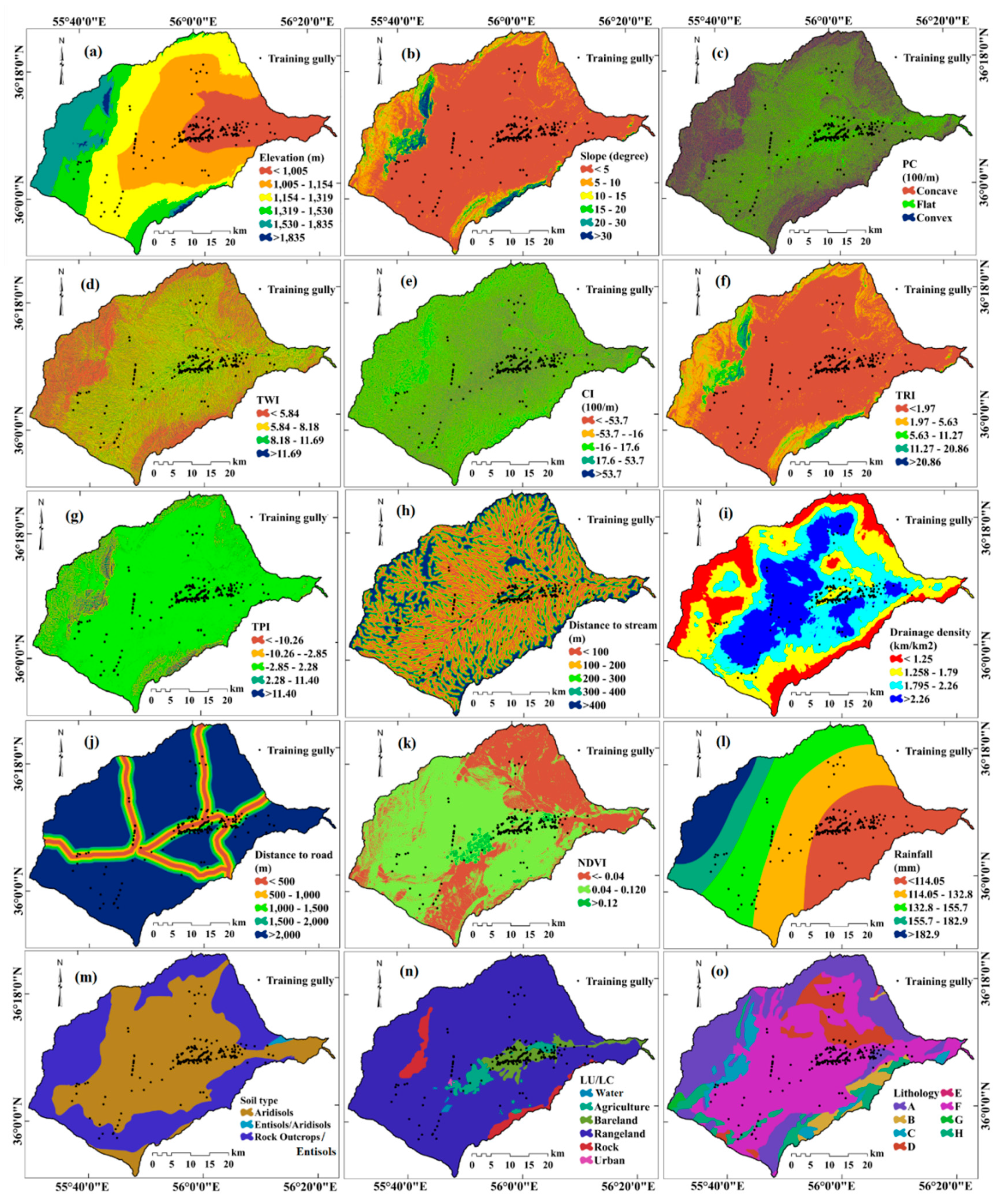
4.2. Spatial Relationship between Conditioning Factors and Gully Locations
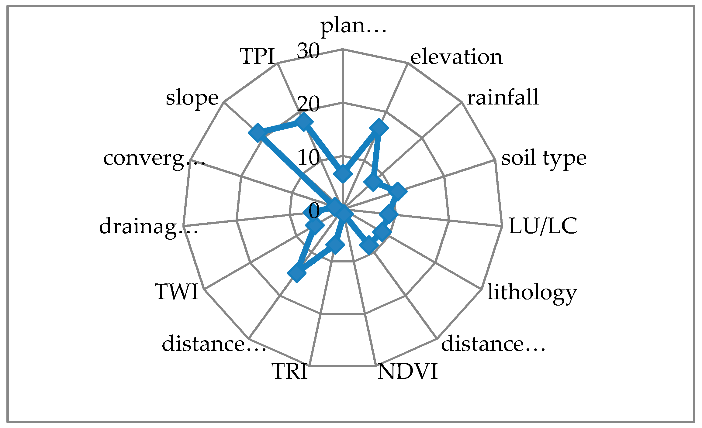
4.3. Relative Importance of Conditioning Factors Using the RF Model
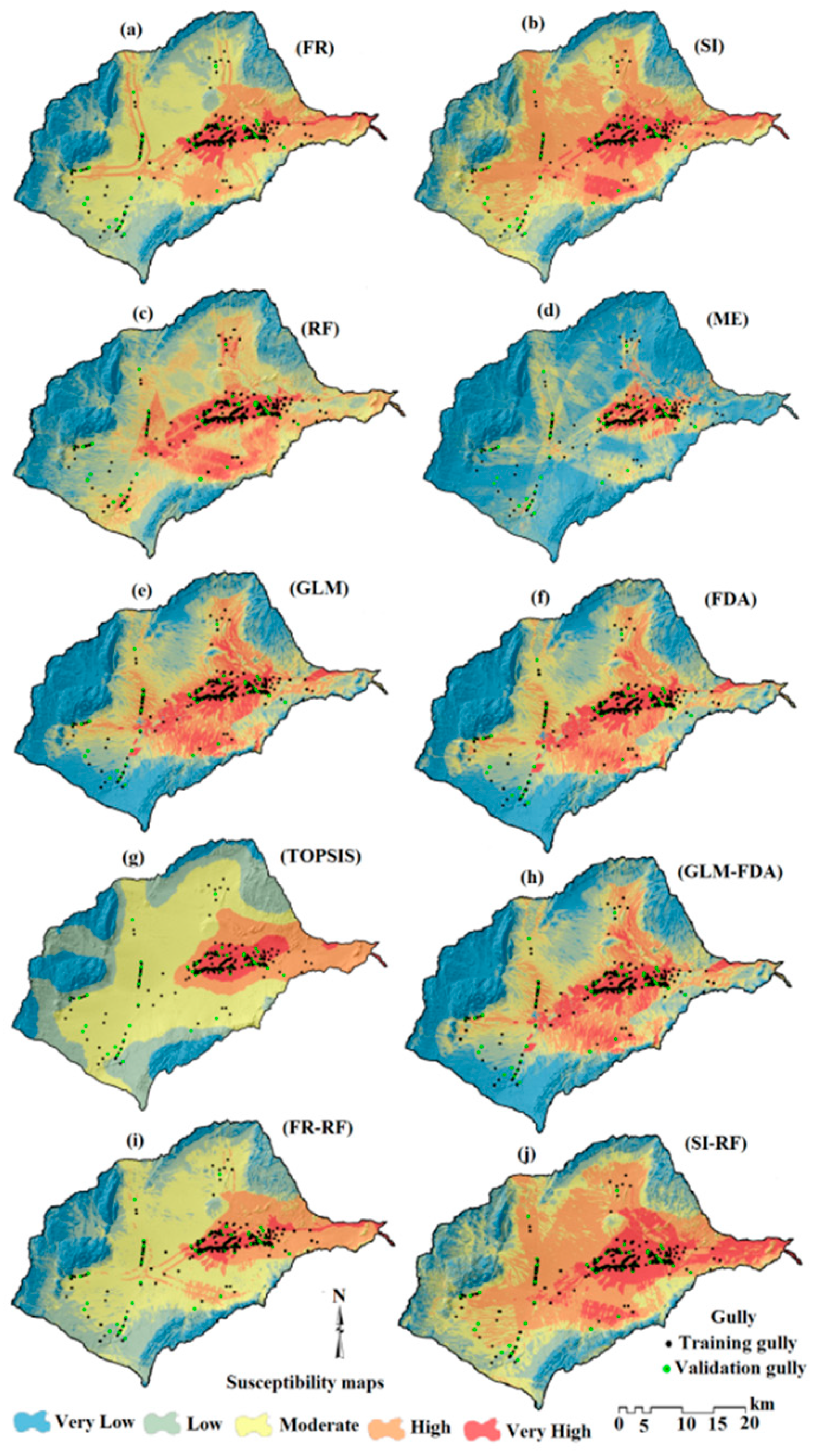
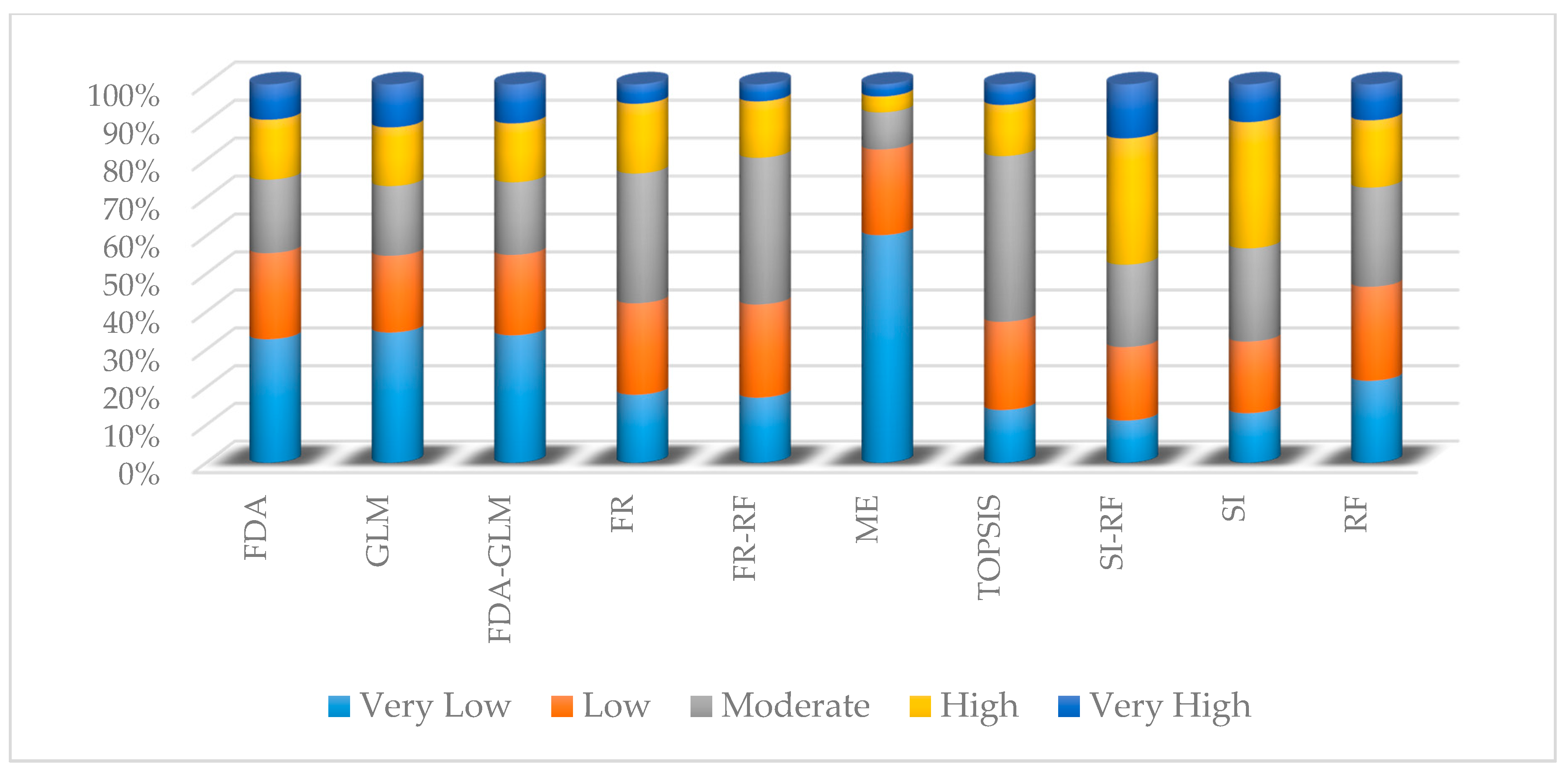
4.4. Gully Erosion Susceptibility Mapping (GESM)
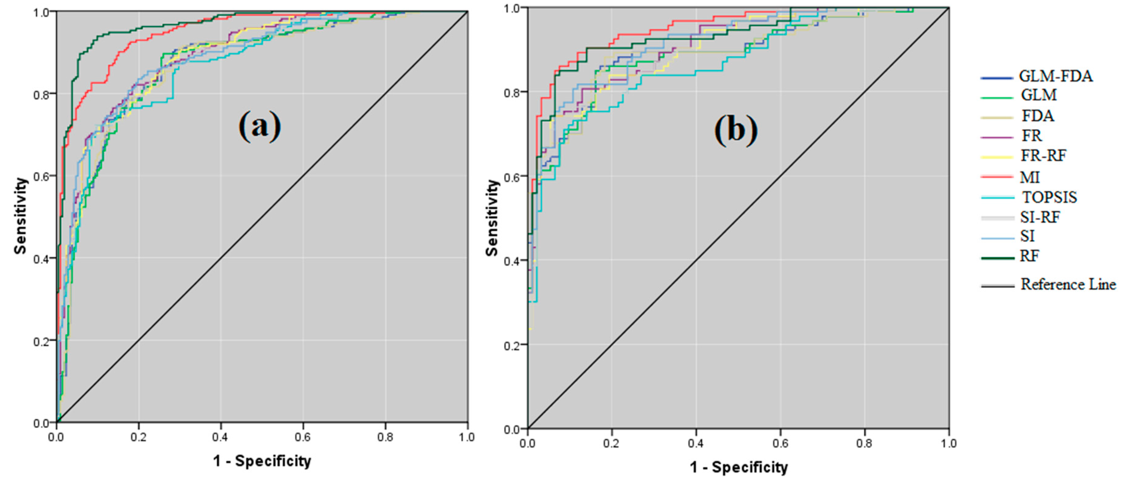
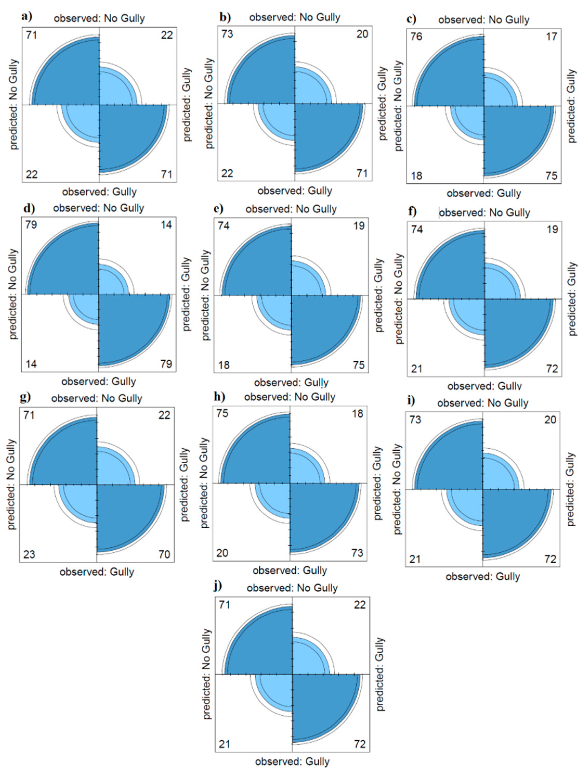
4.5. Validation of Results
5. Discussion
6. Conclusions
Supplementary Materials
Author Contributions
Funding
Conflicts of Interest
References
- Keesstra, S.; Mol, G.; de Leeuw, J.; Okx, J.; de Cleen, M.; Visser, S. Soil-related sustainable development goals: Four concepts to make land degradation neutrality and restoration work. Land 2018, 7, 133. [Google Scholar] [CrossRef]
- Arabameri, A.; Cerda, A.; Rodrigo-Comino, J.; Pradhan, B.; Sohrabi, M.; Blaschke, T.; Tien Bui, D. Proposing a Novel Predictive Technique for Gully Erosion Susceptibility Mapping in Arid and Semi-arid Regions (Iran). Remote Sens. 2019, 11, 2577. [Google Scholar] [CrossRef]
- Arabameri, A.; Pradhan, B.; Rezaei, K.; Yamani, M.; Pourghasemi, H.R.; Lombardo, L. Spatial modelling of gully erosion using Evidential Belief Function, Logistic Regression and a new ensemble EBF–LR algorithm. Land Degrad. Dev. 2018, 29, 4035–4049. [Google Scholar] [CrossRef]
- Arabameri, A.; Chen, W.; Lombardo, L.; Blaschke, T.; Tien Bui, D. Hybrid Computational Intelligence Models for Improvement Gully Erosion Assessment. Remote Sens. 2020, 12, 140. [Google Scholar] [CrossRef]
- Conforti, M.; Aucelli, P.P.; Robustelli, G.; Scarciglia, F. Geomorphology and GIS analysis for mapping gully erosion susceptibility in the Turbolo stream catchment (Northern Calabria, Italy). Nat. Hazards 2011, 56, 881–898. [Google Scholar] [CrossRef]
- Arabameri, A. Application of the Analytic Hierarchy Process (AHP) for locating fire stations: Case Study Maku City. Merit Res. J. Art Soc. Sci. Humanit. 2014, 2, 001–010. [Google Scholar]
- Arabameri, A. Zoning Mashhad Watershed for Artificial Recharge of Underground Aquifers Using TOPSIS Model and GIS Technique. Global Journal of human-social science: B Geography, Geo-Sciences. Environ. Disaster Manag. 2014, 14, 45–53. [Google Scholar]
- Arabameri, A.; Rezaei, K.; Cerda, A.; Conoscenti, C.; Kalantari, Z. A comparison of statistical methods and multi-criteria decision making to map flood hazard susceptibility in Northern Iran. Sci. Total Environ. 2019, 660, 443–458. [Google Scholar] [CrossRef]
- Arabameri, A.; Rezaei, K.; Cerda, A.; Lombardo, L.; Rodrigo-Comino, J. GIS-based groundwater potential mapping in Shahroud plain, Iran. A comparison among statistical (bivariate and multivariate), data mining and MCDM approaches. Sci. Total Environ. 2019, 658, 160–177. [Google Scholar] [CrossRef]
- Yamani, M.; Arabameri, A. Comparison and evaluation of three methods of multi attribute decision making methods in choosing the best plant species for environmental management (Case study: Chah Jam Erg). Nat. Environ. Chang. 2015, 1, 49–62. [Google Scholar]
- Rahmati, O.; Tahmasebipour, N.; Haghizadeh, A.; Pourghasemi, H.R.; Feizizadeh, B. Evaluating the influence of geo-environmental factors on gully erosion in a semi-arid region of Iran: An integrated framework. Sci. Total Environ. 2017, 579, 913–927. [Google Scholar] [CrossRef] [PubMed]
- Meliho, M.; Khattabi, A.; Mhammdi, N. A GIS-based approach for gully erosion susceptibility modelling using bivariate statistics methods in the Ourika watershed, Morocco. Environ. Earth Sci. 2018, 77, 655. [Google Scholar] [CrossRef]
- Zabihi, M.; Mirchooli, F.; Motevalli, A.; Darvishan, A.K.; Pourghasemi, H.R.; Zakeri, M.A.; Sadighi, F. Spatial modelling of gully erosion in Mazandaran Province, northern Iran. Catena 2018, 161, 1–13. [Google Scholar] [CrossRef]
- Hosseinalizadeh, M.; Kariminejad, N.; Rahmati, O.; Keesstra, S.; Alinejad, M.; Behbahani, A.M. How can statistical and artificial intelligence approaches predict piping erosion susceptibility? Sci. Total Environ. 2019, 646, 1554–1566. [Google Scholar] [CrossRef] [PubMed]
- Dube, F.; Nhapi, I.; Murwira, A.; Gumindoga, W.; Goldin, J.; Mashauri, D.A. Potential of weight of evidence modelling for gully erosion hazard assessment in Mbire District—Zimbabwe. Phys. Chem. Earth 2014, 67, 145–152. [Google Scholar] [CrossRef]
- Kornejady, A.; Heidari, K.; Nakhavali, M. Assessment of landslide susceptibility, semi-quantitative risk and management in the Ilam dam basin, Ilam. Iran. Environ. Resour. Res. 2015, 3, 85–109. [Google Scholar]
- Azareh, A.; Rahmati, O.; Rafiei-Sardooi, E.; Sankey, J.B.; Lee, S.; Shahabi, H.; BinAhmad, B. Modelling gully-erosion susceptibility in a semi-arid region, Iran: Investigation of applicability of certainty factor and maximum entropy models. Sci. Total Environ. 2019, 655, 684–696. [Google Scholar] [CrossRef]
- Amiri, M.; Pourghasemi, H.R.; Ghanbarian, G.A.; Afzali, S.F. Assessment of the importance of gully erosion effective factors using Boruta algorithm and its spatial modeling and mapping using three machine learning algorithms. Geoderma 2019, 340, 55–69. [Google Scholar] [CrossRef]
- Rahmati, O.; Tahmasebipour, N.; Haghizadeh, A.; Pourghasemi, H.R.; Feizizadeh, B. Evaluation of different machine learning models for predicting and mapping the susceptibility of gully erosion. Geomorphology 2017, 298, 118–137. [Google Scholar] [CrossRef]
- Gómez-Gutiérrez, Á.; Conoscenti, C.; Angileri, S.E.; Rotigliano, E.; Schnabel, S. Using topographical attributes to evaluate gully erosion proneness (susceptibility) in two mediterranean basins: Advantages and limitations. Natural Hazards 2015, 79, 291–314. [Google Scholar] [CrossRef]
- Hosseinalizadeh, M.; Kariminejad, N.; Chen, W.; Pourghasemi, H.R.; Alinejad, M.; Behbahani, A.M.; Tiefenbacher, J.P. Gully headcut susceptibility modeling using functional trees, naïve Bayes tree, and random forest models. Geoderma 2019, 342, 1–11. [Google Scholar] [CrossRef]
- Arabameri, A.; Pourghasemi, H.R. Spatial Modeling of Gully Erosion Using Linear and Quadratic Discriminant Analyses in GIS and R. In Spatial Modeling in GIS and R for Earth and Environmental Sciences, 1st ed.; Pourghasemi, H.R., Gokceoglu, C., Eds.; Elsevier Publication: Amsterdam, The Netherlands, 2019; 796p. [Google Scholar]
- Hosseinalizadeh, M.; Kariminejad, N.; Chen, W.; Pourghasemi, H.R.; Alinejad, M.; Behbahani, A.M.; Tiefenbacher, J.P. Spatial modelling of gully headcuts using UAV data and four best-first decision classifier ensembles (BFTree, Bag-BFTree, RS-BFTree, and RF-BFTree). Geomorphology 2019, 329, 184–193. [Google Scholar] [CrossRef]
- Pourghasemi, H.R.; Yousefi, S.; Kornejady, A.; Cerdà, A. Performance assessment of individual and ensemble data-mining techniques for gully erosion modeling. Sci. Total Environ. 2017, 609, 764–775. [Google Scholar] [CrossRef] [PubMed]
- Gayen, A.; Pourghasemi, H.R. Spatial Modeling of Gully Erosion: A New Ensemble of CART and GLM Data-Mining Algorithms. In Spatial Modeling in GIS and R for Earth and Environmental Science; Elsevier: Amsterdam, The Netherlands, 2019; pp. 653–669. [Google Scholar]
- Gayen, A.; Pourghasemi, H.R.; Saha, S.; Keesstra, S.; Bai, S. Gully erosion susceptibility assessment and management of hazard-prone areas in India using different machine learning algorithms. Sci. Total Environ. 2019, 668, 124–138. [Google Scholar] [CrossRef]
- Arabameri, A.; Pradhan, B.; Rezaei, K.; Conoscenti, C. Gully erosion susceptibility mapping using GIS-based multi-criteria decision analysis techniques. Catena 2019, 180, 282–297. [Google Scholar] [CrossRef]
- Regmi, A.D.; Devkota, K.C.; Yoshida, K.; Pradhan, B.; Pourghasemi, H.R.; Kumamoto, T.; Akgun, A. Application of frequency ratio, statistical index, and weights-of-evidence models and their comparison in landslide susceptibility mapping in Central Nepal Himalaya. Arab. J. Geosci. 2014, 7, 725–742. [Google Scholar] [CrossRef]
- Van Westen, C.J. Statistical landslide hazard analysis. ILWIS 1997, 2, 73–84. [Google Scholar]
- Chen, W.; Panahi, M.; Khosravi, K.; Pourghasemi, H.R.; Rezaie, F.; Parvinnezhad, D. Spatial prediction of groundwater potentiality using ANFIS ensembled with teaching-learning-based and biogeography-based optimization. J. Hydrol. 2019, 572, 435–448. [Google Scholar] [CrossRef]
- Chen, W.; Pradhan, B.; Li, S.; Shahabi, H.; Rizeei, H.M.; Hou, E.; Wang, S. Novel Hybrid Integration Approach of Bagging-Based Fisher’s Linear Discriminant Function for Groundwater Potential Analysis. Nat. Resour. Res. 2019, 28, 1239–1258. [Google Scholar] [CrossRef]
- Bui, D.T.; Ho, T.C.; Pradhan, B.; Pham, B.T.; Nhu, V.H.; Revhaug, I. GIS-based modeling of rainfall-induced landslides using data mining-based functional trees classifier with AdaBoost, Bagging, and MultiBoost ensemble frameworks. Environ. Earth Sci. 2016, 75, 1101. [Google Scholar]
- Water Resources Company of Semnan (WRCS). Precipitation and Temperature Reports. Available online: http://www.Semnanrw.ir/index.aspx?siteid=1&fkeyid=&siteid=1&pageid=183 (accessed on 21 August 2018).
- Geological Survey Department of Iran (GSDI). 1997. Available online: http://www.gsi.ir/Main/Lang_en/index.html (accessed on 21 August 2018).
- USDA. Keys to soil taxonomy, USDA (United States Department of Agriculture), Soil Survey Staff, 10th ed.; Natural Resources Conservation Service: Washington, DC, USA, 2006; p. 333.
- Arabameri, A.; Chen, W.; Loche, M.; Zhao, X.; Li, Y.; Lombardo, L.; Cerda, A.; Pradhan, B.; Bui, D.T. Comparison of machine learning models for gully erosion susceptibility mapping. Geosci. Front. 2019, in press. [Google Scholar] [CrossRef]
- Ghorbani Nejad, S.; Falah, F.; Daneshfar, M.; Haghizadeh, A.; Rahmati, O. Delineation of groundwater potential zones using remote sensing and GIS-based data-driven models. Geocarto Int. 2016, 32, 167–187. [Google Scholar] [CrossRef]
- Claps, P.; Fiorentino, M.; Oliveto, G. Informational entropy of fractal river networks. J. Hydrol. 1994, 187, 145–156. [Google Scholar] [CrossRef]
- Althuwaynee, O.F.; Pradhan, B.; Park, H.J.; Lee, J.H. A novel ensemble bivariate statistical evidential belief function with knowledge-based analytical hierarchy process and multivariate statistical logistic regression for landslide susceptibility mapping. Catena 2014, 114, 21–36. [Google Scholar] [CrossRef]
- Oh, H.J.; Pradhan, B. Application of a neuro-fuzzy model to landslide-susceptibility mapping for shallow landslides in a tropical hilly area. Comput. Geosci. 2011, 37, 1264–1276. [Google Scholar] [CrossRef]
- Moore, I.D.; Grayson, R.B.; Ladson, A.R. Digital terrain modelling: A review of hydrological, geomorphological, and biological applications. Hydrol. Process 1991, 5, 3–30. [Google Scholar] [CrossRef]
- De Reu, J.; Bourgeois, J.; Bats, M.; Zwertvaegher, A.; Gelorini, V.; De Smedt, P.; Chu, W.; Antrop, M.; De Maeyer, P.; Finke, P.; et al. Application of the topographic position index to heterogeneous landscapes. Geomorphology 2013, 186, 39–49. [Google Scholar] [CrossRef]
- Stotle, J.; Liu, B.; Ritsema, C.J.; Van Den Elsen, H.G.M.; Hessel, R. Modeling water flow and sediment processes in a small gully system on the Loess Plateau in China. Catena 2003, 54, 117–130. [Google Scholar]
- Zinck, J.A.; Lópezb, J.; Metternichtc, G.I.; Shresthaa, D.P.; Vázquez-Selemd, L. Mapping and modelling mass movements and gullies in mountainous areas using remote sensing and GIS techniques. Int. J. Appl. Earth Obs. 2001, 3, 43–53. [Google Scholar] [CrossRef]
- Zakerinejad, R.; Maerker, M. An integrated assessment of soil erosion dynamics with special emphasis on gully erosion in the Mazayjan basin, southwestern Iran. Nat. Hazards 2015, 79, S25–S50. [Google Scholar] [CrossRef]
- Choi, Y.; Park, H.; Sunwoo, C. Flood and gully erosion problems at the Pasir open pit coal mine, Indonesia: A case study of the hydrology using GIS. Bull. Eng. Geol. Environ. 2008, 67, 251–258. [Google Scholar] [CrossRef]
- Nyssen, J.; Poesen, J.; Moeyersons, J.; Luyten, E.; Veyret Picot, M.; Deckers, J.; Mitiku, H.; Govers, G. Impact of road building on gully erosion risk, a case study from the northern Ethiopian highlands. Earth Surf. Process. Landf. 2002, 27, 1267–1283. [Google Scholar] [CrossRef]
- Arabameri, A.; Pradhan, B.; Rezaei, K. Spatial prediction of gully erosion using ALOS PALSAR data and ensemble bivariate and data mining models. Geosci. J. 2019, 23, 669–686. [Google Scholar] [CrossRef]
- Lucà, F.; Conforti, M.; Robustelli, G. Comparison of GIS-based gullying susceptibility mapping using bivariate and multivariate statistics: Northern Calabria, South Italy. Geomorphology 2011, 134, 297–308. [Google Scholar] [CrossRef]
- Arabameri, A.; Cerda, A.; Tiefenbacher, J.P. Spatial pattern analysis and prediction of gully erosion using novel hybrid model of entropy-weight of evidence. Water 2019, 11, 1129. [Google Scholar] [CrossRef]
- Rahmati, O.; Haghizadeh, A.; Pourghasemi, H.R.; Noormohamadi, F. Gully erosion susceptibility mapping: The role of GIS based bivariate statistical models and their comparison. Nat. Hazards 2016, 82, 1231–1258. [Google Scholar] [CrossRef]
- Arabameri, A.; Pradhan, B.; Rezaei, K. Gully erosion zonation mapping using integrated geographically weighted regression with certainty factor and random forest models in GIS. J. Environ. Manag. 2019, 232, 928–942. [Google Scholar] [CrossRef]
- Hong, H.; Kornejady, A.; Soltani, A.; Termeh, S.V.R.; Liu, J.; Zhu, A.X.; Hesar, A.Y.; Ahmad, B.B.; Wang, Y.C. Landslide susceptibility assessment in the Anfu County, China: Comparing different statistical and probabilistic models considering the new topo-hydrological factor (HAND). Earth Sci. Inf. 2018, 11, 605–622. [Google Scholar] [CrossRef]
- Mandal, S.; Mandal, K. Bivariate statistical index for landslide susceptibility mapping in the Rorachu river basin of eastern Sikkim Himalaya, India. Spat. Inf. Res. 2018, 26, 59–75. [Google Scholar] [CrossRef]
- Nicu, I.C. Application of analytic hierarchy process, frequency ratio, and statistical index to landslide susceptibility: An approach to endangered cultural heritage. Environ. Earth Sci. 2018, 77, 79. [Google Scholar] [CrossRef]
- Aditian, A.; Kubota, T.; Shinohara, Y. Comparison of GIS-based landslide susceptibility models using frequency ratio, logistic regression, and artificial neural network in a tertiary region of Ambon, Indonesia. Geomorphology 2018, 318, 101–111. [Google Scholar] [CrossRef]
- Breiman, L. Random Forests; Statistics Department, University of California: Berkeley, CA USA, 2011. [Google Scholar]
- Cutler, D.R.; Edwards, T.C.; Beard, K.H.; Cutler, A.; Hess, K.T.; Gibson, J.; Lawler, J.J. Random forests for classification in ecology. Ecology 2007, 88, 2783–2792. [Google Scholar] [CrossRef] [PubMed]
- Breiman, L.; Cutler, A. Breiman and Cutler’s Random Forests for Classification and Regression, 1st ed. 2018. Available online: https://www.stat.berkeley.edu/~breiman/RandomForests/ (accessed on 25 August 2018).
- Pourghasemi, H.R.; Kerle, N. Random forests and evidential belief function-based landslide susceptibility assessment in Western Mazandaran Province, Iran. Environ. Earth Sci. 2016, 75, 185. [Google Scholar] [CrossRef]
- Woodbury, A.; Render, F.; Ulrych, T. Practical probabilistic groundwater modeling. Groundwater 1995, 33, 532–538. [Google Scholar] [CrossRef]
- Phillips, S.; Anderson, R.; Schapire, R. Maximum entropy modelling of species geo- graphic distributions. Ecol. Model. 2006, 190, 231–259. [Google Scholar] [CrossRef]
- Harremoës, P.; Topsøe, F. Maximum entropy fundamentals. Entropy 2001, 3, 191–226. [Google Scholar] [CrossRef]
- Ahmedou, A.; Marion, J.-M.; Pumo, B. Generalized linear model with functional predictors and their derivatives. J. Multivar. Anal. 2016, 146, 313–324. [Google Scholar] [CrossRef]
- Naimi, B.; Araújo, M.B. sdm: A reproducible and extensible R platform for species distribution modelling. Ecography 2016, 39, 368375. [Google Scholar] [CrossRef]
- Ramsay, J.; Dalzell, C.J. Some tools for functional data analysis (with discussion). J. R. Statist. Soc. B 1991, 53, 539–572. [Google Scholar]
- Seifi Majdar, R.; Ghassemian, H. Spectral-spatial classification of hyperspectral images using functional data analysis. Remote Sens. Lett. 2017, 8, 488–497. [Google Scholar] [CrossRef]
- Hwang, C.L.; Yoon, N. Multiple Attributes Decision Making Methods and Application, 1st ed.; Springer: Berlin, Germany, 1981. [Google Scholar] [CrossRef]
- Olson, D.L. Comparison of weights in TOPSIS models. Math. Comput. Model 2004, 40, 21–727. [Google Scholar] [CrossRef]
- Pourghasemi, H.R.; Rossi, M. Landslide susceptibility modeling in a landslide prone area in Mazandarn Province, north of Iran: A comparison between GLM, GAM, MARS, and M-AHP methods. Theor. Appl. Climatol. 2017, 130, 609–633. [Google Scholar] [CrossRef]
- Cama, M.; Lombardo, L.; Conoscenti, C.; Rotigliano, E. Improving transferability strategies for debris flow susceptibility assessment: Application to the Saponara and Itala catchments (Messina, Italy). Geomorphology 2017, 288, 52–65. [Google Scholar] [CrossRef]
- Arabameri, A.; Pradhan, B.; Lombardo, L. Comparative assessment using boosted regression trees, binary logistic regression, frequency ratio and numerical risk factor for gully erosion susceptibility modelling. Catena 2019, 183, 104223. [Google Scholar] [CrossRef]
- Razavizadeh, S.; Solaimani, K.; Massironi, M.; Kavian, A. Mapping landslide susceptibility with frequency ratio, statistical index, and weights of evidence models: A case study in Northern Iran. Environ. Earth Sci. 2017, 76, 499. [Google Scholar] [CrossRef]
- Liu, J.; Duan, Z. Quantitative Assessment of Landslide Susceptibility Comparing Statistical Index, Index of Entropy, andWeights of Evidence in the Shangnan Area, China. Entropy 2018, 20, 868. [Google Scholar] [CrossRef]
- Arabameri, A.; Abbasi, S.; Eftekhari, S.M.; Amouniya, H. Selection the Most Suitable Species type for stabiliting sand dunes in dealing with the spread of desertification for environmental sustainability using TOPSIS method (Case study: Chah Jam Erg in South of Haj Ali Gholi Playa in Central part of Semnan Province, Iran). Petroleum Geosci. 2014, 70, 23793–23798. [Google Scholar]
- Arabameri, A.; Pourghasemi, H.R.; Cerda, A. Erodibility prioritization of sub-watersheds using morphometric parameters analysis and its mapping: A comparison among TOPSIS, VIKOR, SAW, and CF multi-criteria decision making models. Sci. Total Environ. 2017, 613–614, 1385–1400. [Google Scholar]
- Beullens, J.; Van de Velde, D.; Nyssen, J. Impact of slope aspect on hydrological rain-fall and on the magnitude of rill erosion in Belgium and northern France. Catena 2014, 114, 129–139. [Google Scholar] [CrossRef]
- Pelletier, J.D.; Barron-Gafford, G.A.; Breshears, D.D.; Brooks, P.D.; Chorover, J.; Durcik, M.; Wagner-Muns, I.M.; Guardiola, I.G.; Samaranayke, V.A.; Kayani, W.I. A Functional data analysis approach to traffic volume forecasting. IEEE Trans. Intell. Transp. Syst. 2018, 19, 878888. [Google Scholar]
- Agnesi, V.; Angileri, S.; Cappadonia, C.; Conoscenti, C.; Rotigliano, E. Multi-parametric GIS analysis to assess gully erosion susceptibility: A test in southern Sicily, Italy. Landf. Anal. 2011, 7, 15–20. [Google Scholar]
- Harvey, A.M. The role of piping in the development of badlands and gully systems in south-east Spain. In Badland Geomorphology and Piping; Bryan, R., Yair, A., Eds.; Geobooks: Norwich, UK, 1982; pp. 317–335. [Google Scholar]
- Valentin, C.; Poesen, J.; Li, Y. Gully erosion: Impacts, factors and control. Catena 2005, 63, 132–153. [Google Scholar] [CrossRef]
- Arabameri, A.; Pradhan, B.; Pourghasemi, H.R.; Rezaei, K.; Kerle, N. Spatial Modelling of Gully Erosion Using GIS and R Programing: A Comparison among Three Data Mining Algorithms. Appl. Sci. 2018, 8, 1369. [Google Scholar] [CrossRef]
- Conoscenti, C.; Angileri, S.; Cappadonia, C.; Rotigliano, E.; Agnesi, V.; Märker, M. Gully erosion susceptibility assessment by means of GIS-based logistic regression: A case of Sicily (Italy). Geomorphology 2014, 204, 399–411. [Google Scholar] [CrossRef]
- Belayneh, L.; Bantider, A.; Moges, A. Road construction and gully development in Hadero Tunto-Durgi road project, Southern Ethopia. Ethiop. J. Environ. Stud. Manag. 2014, 7, 720–730. [Google Scholar] [CrossRef]
- Shellberg, J.G.; Spencer, J.; Brooks, A.P.; Pietsch, T.J. Degradation of the Mitchell Riverfluvialmegafan by alluvial gully erosion increased by post-European land use change, Queensland, Australia. Geomorphology 2016, 266, 105–120. [Google Scholar] [CrossRef]
- Nyssen, J.; Poesen, J.; Moeyersons, J.; Luyten, E.; Veyret-Picot, M.; Deckers, J.; Haile, M.; Svoray, T.; Markovitch, H. Catchment scale analysis of the effect of topography, tillage direction and unpaved roads on ephemeral gully incision. Earth Surf. Process Landf. 2009, 34, 1970–1984. [Google Scholar]
- Cevik, E.; Topal, T. GIS-based landslide susceptibility mapping for a problematic segment of the natural gas pipeline, Hendek (Turkey). Environ. Geol. 2003, 44, 949–962. [Google Scholar] [CrossRef]
- Arabameri, A.; Rezaei, K.; Pourghasemi, H.R.; Lee, S.; Yamani, M. GIS-based gully erosion susceptibility mapping: A comparison among three data-driven models and AHP knowledge-based technique. Environ. Earth Sci. 2018, 77, 628. [Google Scholar] [CrossRef]
- Dickie, J.A.; Parsons, A.J. Eco-geomorphological processes within grasslands, shrub lands and badlands in the semi-arid Karoo, South Africa. Land Degrad. Dev. 2012, 23, 534–547. [Google Scholar] [CrossRef]
- Zucca, C.; Canu, A.; Della Peruta, R. Effects of land use and landscape on spatial distribution and morphological features of gullies in an agropastoral area in Sardinia (Italy). Catena 2006, 68, 87–95. [Google Scholar] [CrossRef]
- Arabameri, A.; Chen, W.; Blaschke, T.; Tiefenbacher, J.P.; Pradhan, B.; Tien Bui, D. Gully Head-Cut Distribution Modeling Using Machine Learning Methods—A Case Study of N.W. Iran. Water 2020, 12, 16. [Google Scholar] [CrossRef]
- Zhang, G.S.; Chan, K.Y.; Oates, A.; Heenan, D.P.; Huang, G.B. Relationship between soil structure and runoff/soil loss after 24 years of conservation tillage. Soil Tillage Res. 2007, 92, 122–128. [Google Scholar] [CrossRef]
- García-Ruiz, J.M. The effects of land uses on soil erosion in Spain: A review. Catena 2010, 81, 1–11. [Google Scholar] [CrossRef]
- Poesen, J.; Nachtergaele, J.; Verstraeten, G.; Valentin, C. Gully erosion and environmental change: Importance and research needs. Catena 2003, 50, 91–133. [Google Scholar] [CrossRef]
- Garosi, Y.; Sheklabadi, M.; Pourghasemi, H.R.; Besalatpour, A.A.; Conoscenti, C.; Van Oost, K. Comparison of differences in resolution and sources of controlling factors for gully erosion susceptibility mapping. Geoderma 2018, 330, 65–78. [Google Scholar] [CrossRef]
- Kim, J.C.; Lee, S.; Jung, H.S.; Lee, S. Landslide susceptibility mapping using random forest and boosted tree models in Pyeong-Chang, Korea. Geocato Int. 2018, 33, 1000–1015. [Google Scholar] [CrossRef]
- Kantardzic, M. Data Mining: Concepts, Models, Methods, and Algorithms, 2nd ed.; John Wiley & Sons, Inc.: Hoboken, NJ, USA, 2004. [Google Scholar]
- Lombardo, L.; Bachofer, F.; Cama, M.; Märker, M.; Rotigliano, E. Exploiting Maximum Entropy method and ASTER data for assessing debris flow and debris slide suscepti- bility for the Giampilieri catchment (north-eastern Sicily, Italy). Earth Surf. Process. Landf. 2016, 41, 1776–1789. [Google Scholar] [CrossRef]
- Pandey, V.K.; Pourghasemi, H.R.; Sharma, M.C. Landslide susceptibilitymappingusing maximum entropy and support vector machine models along the Highway Corridor, Garhwal Himalaya. Geocarto Int. 2018. [Google Scholar] [CrossRef]
- Siahkamari, S.; Haghizadeh, A.; Zeinivand, H.; Tahmasebipour, N.; Rahmati, O. Spatial prediction of flood-susceptible areas using frequency ratio and maximum en- tropy models. Geocarto Int. 2018, 33, 927–941. [Google Scholar] [CrossRef]
- Tan, L.; Taniar, D. Adaptive estimated maximum-entropy distribution model. Inf. Sci. 2007, 177, 3110–3128. [Google Scholar] [CrossRef]
- Genuer, R.; Poggi, J.-M.; Tuleau-Malot, C.; Villa-Vialaneix, N. Random forests for big data. Big Data Res. 2017, 9, 28–46. [Google Scholar] [CrossRef]
- Kornejady, A.; Pourghasemi, H.R.; Afzali, S.F. Presentation of RFFR New Ensemble Model for Landslide Susceptibility Assessment in Iran. In Landslides: Theory, Practice and Modelling. Advances in Natural and Technological Hazards Research; Pradhan, S., Vishal, V., Singh, T., Eds.; Springer: Cham, Switzerland, 2019; Volume 50. [Google Scholar]


| No. | Factor | Classes | Classification Method | References |
|---|---|---|---|---|
| 1 | Elevation (m) | 1. <1005, 2. 1005–1154, 33. 1154–1319, 4. 1319–1530, 5. 1530–1835, 6. >1835 | Natural break | [48] |
| 2 | Slope (°) | 1. <5, 2. 5–10, 3. 10–15, 4. 15–20, 5. 20–30, 6. >30 | Manual | [49] |
| 3 | Plan curvature (m−1) | 1. Concave, 2. Flat, 3. Convex | Manual | [48] |
| 4 | TWI | 1. <5.84, 2. 5.84–8.18, 3. 8.18–11.69, 4. >11.69 | Natural break | [48] |
| 5 | CI | 1. <–53.7, 2. −53.7–−16, 3. −16–17.6, 4. 17.6–53.7, 5. >53.7 | Natural break | [48] |
| 6 | TRI (m) | 1. <1.97, 2. 1.97–5.63, 3. 5.63–11.27, 4. 11.27–20.86, 5. >20.86 | Natural break | [50] |
| 7 | TPI | 1. <−10.26, 2. −10.26–−2.85, 3. −2.85–2.28, 4. 2.28–11.4, 5. > 11.4 | Natural break | [50] |
| 8 | Distance to river (m) | 1. <100, 2. 100–200, 3. 200–300, 4. 300–400, 5. >400 | Manual | [48] |
| 9 | Drainage density (km/km2) | 1. < 1.25, 2. 1.25–1.79, 3. 1.79–2.26, 4. >2.26 | Natural break | [51] |
| 10 | Distance to road (m) | 1. <500, 2. 500–1000, 3. 1000–1500, 4. 1500–2000, 5. >2000 | Manual | [52] |
| 11 | NDVI | 1. <−0.04, 2. −0.04–0.12, 3. >0.12 | Natural break | [48] |
| 12 | Rainfall | 1. <114.05, 2.114.05–132.8, 3. 132.8–155.7, 4. 155.7–182.9, 5. <182.9 | Natural break | [48] |
| 13 | Soil | 1. Rock Outcrops/Entisols, 2. Aridisols, 3. Entisols/Aridisols | Soil type | |
| 14 | LULC | 1. Abkhan, 2. Agriculture, 3. Bareland, 4. Rangeland, 5. Rock, 6. Urban | Land use type | |
| 15 | Lithology | 1. A, 2. B, 3. C, 4. D, 5. E, 6. F, 7. G, 8. H | Lithology type |
| * Factors | Unstandardized Coefficients | Standardized Coefficients | t | Sig. | Collinearity Statistics | ||
|---|---|---|---|---|---|---|---|
| B | Std. Error | Beta | Tolerance | VIF | |||
| (Constant) | −0.272 | 0.164 | −1.666 | 0.096 | |||
| lithology | −0.006 | 0.038 | −0.007 | −0.159 | 0.874 | 0.554 | 1.805 |
| LU/LC | 0.016 | 0.005 | 0.164 | 3.033 | 0.003 | 0.415 | 2.412 |
| Soil type | 0.083 | 0.037 | 0.104 | 2.205 | 0.028 | 0.546 | 1.831 |
| Drainage density | 0.073 | 0.029 | 0.107 | 2.517 | 0.012 | 0.672 | 1.489 |
| Rainfall | 0.002 | 0.029 | 0.005 | 0.076 | 0.939 | 0.245 | 4.078 |
| Slope | 0.143 | 0.110 | 0.092 | 1.296 | 0.196 | 0.241 | 4.153 |
| TRI | −0.079 | 0.108 | −0.055 | −0.729 | 0.466 | 0.214 | 4.668 |
| TPI | 0.048 | 0.079 | 0.027 | 0.601 | 0.548 | 0.586 | 1.706 |
| TWI | −0.082 | 0.059 | −0.055 | −1.404 | 0.161 | 0.784 | 1.276 |
| PC | 0.054 | 0.106 | 0.019 | 0.506 | 0.613 | 0.903 | 1.108 |
| NDVI | 0.102 | 0.040 | 0.107 | 2.526 | 0.012 | 0.685 | 1.459 |
| Dis to stream | 0.126 | 0.041 | 0.116 | 3.084 | 0.002 | 0.863 | 1.158 |
| Dis to road | 0.080 | 0.013 | 0.263 | 6.148 | 0.000 | 0.666 | 1.501 |
| elevation | 0.055 | 0.020 | 0.202 | 2.815 | 0.005 | 0.237 | 4.224 |
| CI | −0.070 | 0.085 | −0.029 | −0.818 | 0.414 | 0.940 | 1.063 |
| * Factor | Class | Pixels in Domain | Gullies | FR | SI | ||
|---|---|---|---|---|---|---|---|
| No | % | No | % | ||||
| Elevation (m) | <1005 | 409583 | 16.47 | 143 | 67.45 | 4.09 | 1.41 |
| 1005–1154 | 778,768 | 31.32 | 45 | 21.23 | 0.68 | −0.39 | |
| 1154–1319 | 675,092 | 27.15 | 17 | 8.02 | 0.30 | −1.22 | |
| 1319–1530 | 314,348 | 12.64 | 7 | 3.30 | 0.26 | −1.34 | |
| 1530–1835 | 290,378 | 11.68 | 0 | 0.00 | 0.00 | None | |
| >1835 | 18,056 | 0.73 | 0 | 0.00 | 0.00 | None | |
| Slope (°) | <5 | 2,018,483 | 81.19 | 205 | 96.70 | 1.19 | 0.17 |
| 5–10 | 235,497 | 9.47 | 7 | 3.30 | 0.35 | −1.05 | |
| 10–15 | 98,979 | 3.98 | 0 | 0.00 | 0.00 | None | |
| 15–20 | 46,006 | 1.85 | 0 | 0.00 | 0.00 | None | |
| 20–30 | 44,839 | 1.80 | 0 | 0.00 | 0.00 | None | |
| >30 | 42,421 | 1.71 | 0 | 0.00 | 0.00 | None | |
| PC (100/m) | Concave | 792,994 | 31.90 | 55 | 25.94 | 0.81 | −0.21 |
| Flat | 907,578 | 36.50 | 94 | 44.34 | 1.21 | 0.19 | |
| Convex | 785,652 | 31.60 | 63 | 29.72 | 0.94 | −0.06 | |
| TWI | <5.84 | 805,518 | 32.40 | 33 | 15.57 | 0.48 | −0.73 |
| 5.84–8.18 | 1,120,812 | 45.08 | 123 | 58.02 | 1.29 | 0.25 | |
| 8.18–11.69 | 408,848 | 16.44 | 38 | 17.92 | 1.09 | 0.09 | |
| >11.69 | 151,046 | 6.08 | 18 | 8.49 | 1.40 | 0.33 | |
| CI (100/m) | <−53.7 | 170,770 | 6.98 | 16 | 7.55 | 1.08 | 0.08 |
| −53.7–−16 | 614,268 | 25.10 | 44 | 20.75 | 0.83 | −0.19 | |
| −16–17.6 | 994,363 | 40.63 | 83 | 39.15 | 0.96 | −0.04 | |
| 17.6–53.7 | 535,208 | 21.87 | 54 | 25.47 | 1.16 | 0.15 | |
| >53.7 | 133,049 | 5.44 | 15 | 7.08 | 1.30 | 0.26 | |
| TRI | <1.97 | 1,995,829 | 80.28 | 207 | 97.64 | 1.22 | 0.20 |
| 1.97–5.63 | 314,118 | 12.63 | 5 | 2.36 | 0.19 | −1.68 | |
| 5.63–11.27 | 120,287 | 4.84 | 0 | 0.00 | 0.00 | None | |
| 11.27–20.86 | 45,815 | 1.84 | 0 | 0.00 | 0.00 | None | |
| >20.86 | 10,176 | 0.41 | 0 | 0.00 | 0.00 | None | |
| TPI | <−10.26 | 27,479 | 1.11 | 0 | 0.00 | 0.00 | None |
| −10.26–−2.85 | 202,970 | 8.16 | 5 | 2.36 | 0.29 | −1.24 | |
| −2.85–2.28 | 2,103,205 | 84.59 | 207 | 97.64 | 1.15 | 0.14 | |
| 2.28–11.4 | 130,891 | 5.26 | 0 | 0.00 | 0.00 | None | |
| >11.4 | 21,679 | 0.87 | 0 | 0.00 | 0.00 | None | |
| Dis to stream (m) | <100 | 881,433 | 35.45 | 117 | 55.19 | 1.56 | 0.44 |
| 100–200 | 625,868 | 25.17 | 54 | 25.47 | 1.01 | 0.01 | |
| 200–300 | 443,260 | 17.83 | 25 | 11.79 | 0.66 | −0.41 | |
| 300–400 > 400 | 224,458 311,205 | 9.03 12.52 | 10 6 | 4.72 2.83 | 0.52 0.23 | −0.65 −1.49 | |
| Drainage density (km/km2) | <1.25 | 461689 | 18.57 | 2 | 0.94 | 0.05 | −2.98 |
| 1.25–1.79 | 746549 | 30.03 | 55 | 25.94 | 0.86 | −0.15 | |
| 1.79–2.26 | 712235 | 28.65 | 124 | 58.49 | 2.04 | 0.71 | |
| >2.26 | 565752 | 22.76 | 31 | 14.62 | 0.64 | −0.44 | |
| Dis to road (m) | <500 | 177023 | 7.12 | 32 | 15.09 | 2.12 | 0.75 |
| 500–1000 | 168791 | 6.79 | 68 | 32.08 | 4.72 | 1.55 | |
| 1000–1500 | 159125 | 6.40 | 31 | 14.62 | 2.28 | 0.83 | |
| 1500–2000 | 151080 | 6.08 | 26 | 12.26 | 2.02 | 0.70 | |
| > 2000 | 1830206 | 73.61 | 55 | 25.94 | 0.35 | −1.04 | |
| NDVI | <−0.04 | 918021 | 36.92 | 17 | 8.02 | 0.22 | −1.53 |
| −0.04–0.12 | 1541694 | 62.01 | 192 | 90.57 | 1.46 | 0.38 | |
| >0.12 | 26510 | 1.07 | 3 | 1.42 | 1.33 | 0.28 | |
| Rainfall (mm) | <114.05 | 688309 | 27.68 | 161 | 75.94 | 2.74 | 1.01 |
| 114.05–132.8 | 694011 | 27.91 | 21 | 9.91 | 0.35 | −1.04 | |
| 132.8–155.7 | 619724 | 24.93 | 23 | 10.85 | 0.44 | −0.83 | |
| 155.7–182.9 | 259107 | 10.42 | 7 | 3.30 | 0.32 | −1.15 | |
| <182.9 | 225074 | 9.05 | 0 | 0.00 | 0.00 | None | |
| Soil type | Rock Outcrops/Entisols | 1035170 | 41.64 | 12 | 5.66 | 0.14 | −2.00 |
| Aridisols | 1443591 | 58.06 | 199 | 93.87 | 1.62 | 0.48 | |
| Entisols/Aridisols | 7464 | 0.30 | 1 | 0.47 | 1.57 | 0.45 | |
| LU/LC | Abkhan | 5419 | 0.22 | 0 | 0.00 | 0.00 | None |
| Agriculture | 73837 | 2.97 | 11 | 5.19 | 1.75 | 0.56 | |
| Bareland | 124293 | 5.00 | 124 | 58.49 | 11.70 | 2.46 | |
| Rangeland | 2182822 | 87.80 | 76 | 35.85 | 0.41 | −0.90 | |
| Rock | 98132 | 3.95 | 1 | 0.47 | 0.12 | −2.12 | |
| Urban | 1722 | 0.07 | 0 | 0.00 | 0.00 | None | |
| Lithology | A | 697041 | 28.04 | 20 | 9.43 | 0.34 | −1.09 |
| B | 79375 | 3.19 | 1 | 0.47 | 0.15 | −1.91 | |
| C | 114582 | 4.61 | 3 | 1.42 | 0.31 | −1.18 | |
| D | 190539 | 7.66 | 10 | 4.72 | 0.62 | −0.49 | |
| E | 2747 | 0.11 | 0 | 0.00 | 0.00 | None | |
| F | 153705 | 6.18 | 4 | 1.89 | 0.31 | −1.19 | |
| G | 1236071 | 49.72 | 174 | 82.08 | 1.65 | 0.50 | |
| H | 12165 | 0.49 | 0 | 0.00 | 0.00 | None | |
| * Models | Classification with a Natural Break Model | ||||
|---|---|---|---|---|---|
| Very Low | Low | Moderate | High | Very High | |
| FR | 3.66–9.63 | 9.63–13.79 | 13.79–17.96 | 17.96–26.57 | 26.57–39.06 |
| SI | −19.3–−10.5 | −10.5–−6 | −6–−2.27 | −2.27–2.25 | 2.25–10.25 |
| RF | 0.01–0.21 | 0.21–0.37 | 0.37–0.53 | 0.53–0.72 | 0.72–1 |
| ME | 0.00–0.06 | 0.06–0.17 | 0.17–0.34 | 0.34–0.57 | 0.57–0.97 |
| GLM | 0.00–0.12 | 0.12–0.3 | 0.3–0.49 | 0.49–0.69 | 0.69–0.98 |
| FDA | 0.00–0.13 | 0.13–0.31 | 0.31–0.51 | 0.51–0.73 | 0.73–0.99 |
| TOPSIS | 0.15–0.29 | 0.29–0.38 | 0.38–0.48 | 0.48–0.61 | 0.61–0.78 |
| GLM-FDA | 0.00–0.13 | 0.13–0.31 | 0.31–0.5 | 0.5–0.71 | 0.71–0.99 |
| FR-RF | 21.72–84.7 | 84.7–131.2 | 131.2–183.2 | 183.2–268.1 | 268.1–370.8 |
| SI-RF | −190–−99.9 | −99.9–−59.3 | −59.3–−23.2 | −23.2–18.4 | 18.4–97.4 |
| * Criteria | TN | FP | FN | TP | TPR | TNR | FPR | Cutoff-Dependent Criteria | Cutoff Independent Criteria | |||
|---|---|---|---|---|---|---|---|---|---|---|---|---|
| * Models | AUSRC | AUPRC | Aaccuracy | Kappa | ||||||||
| FR | 71 | 22 | 22 | 71 | 0.76 | 0.76 | 0.23 | 0.890 | 0.900 | 0.763 | 0.527 | |
| SI | 73 | 20 | 22 | 71 | 0.76 | 0.78 | 0.21 | 0.884 | 0.897 | 0.774 | 0.548 | |
| RF | 76 | 17 | 18 | 75 | 0.80 | 0.81 | 0.18 | 0.965 | 0.932 | 0.812 | 0.624 | |
| ME | 79 | 14 | 14 | 79 | 0.84 | 0.84 | 0.15 | 0.947 | 0.948 | 0.849 | 0.699 | |
| GLM | 74 | 19 | 18 | 75 | 0.80 | 0.79 | 0.20 | 0.869 | 0.887 | 0.801 | 0.602 | |
| FDA | 74 | 19 | 21 | 72 | 0.77 | 0.79 | 0.20 | 0.868 | 0.894 | 0.785 | 0.570 | |
| TOPSIS | 71 | 22 | 23 | 70 | 0.75 | 0.76 | 0.23 | 0.871 | 0.867 | 0.758 | 0.516 | |
| GLM-FDA | 75 | 18 | 20 | 73 | 0.78 | 0.80 | 0.19 | 0.870 | 0.891 | 0.796 | 0.591 | |
| FR-RF | 73 | 20 | 21 | 72 | 0.77 | 0.78 | 0.21 | 0.893 | 0.908 | 0.780 | 0.559 | |
| SI-RF | 71 | 22 | 21 | 72 | 0.77 | 0.76 | 0.237 | 0.889 | 0.914 | 0.769 | 0.538 | |
© 2020 by the authors. Licensee MDPI, Basel, Switzerland. This article is an open access article distributed under the terms and conditions of the Creative Commons Attribution (CC BY) license (http://creativecommons.org/licenses/by/4.0/).
Share and Cite
Arabameri, A.; Blaschke, T.; Pradhan, B.; Pourghasemi, H.R.; Tiefenbacher, J.P.; Bui, D.T. Evaluation of Recent Advanced Soft Computing Techniques for Gully Erosion Susceptibility Mapping: A Comparative Study. Sensors 2020, 20, 335. https://doi.org/10.3390/s20020335
Arabameri A, Blaschke T, Pradhan B, Pourghasemi HR, Tiefenbacher JP, Bui DT. Evaluation of Recent Advanced Soft Computing Techniques for Gully Erosion Susceptibility Mapping: A Comparative Study. Sensors. 2020; 20(2):335. https://doi.org/10.3390/s20020335
Chicago/Turabian StyleArabameri, Alireza, Thomas Blaschke, Biswajeet Pradhan, Hamid Reza Pourghasemi, John P. Tiefenbacher, and Dieu Tien Bui. 2020. "Evaluation of Recent Advanced Soft Computing Techniques for Gully Erosion Susceptibility Mapping: A Comparative Study" Sensors 20, no. 2: 335. https://doi.org/10.3390/s20020335
APA StyleArabameri, A., Blaschke, T., Pradhan, B., Pourghasemi, H. R., Tiefenbacher, J. P., & Bui, D. T. (2020). Evaluation of Recent Advanced Soft Computing Techniques for Gully Erosion Susceptibility Mapping: A Comparative Study. Sensors, 20(2), 335. https://doi.org/10.3390/s20020335