Variational Bayesian Pansharpening with Super-Gaussian Sparse Image Priors

Abstract

Pansharpening is a technique that fuses a low spatial resolution multispectral image and a high spatial resolution panchromatic one to obtain a multispectral image with the spatial resolution of the latter while preserving the spectral information of the multispectral image. In this paper we propose a variational Bayesian methodology for pansharpening. The proposed methodology uses the sensor characteristics to model the observation process and Super-Gaussian sparse image priors on the expected characteristics of the pansharpened image. The pansharpened image, as well as all model and variational parameters, are estimated within the proposed methodology. Using real and synthetic data, the quality of the pansharpened images is assessed both visually and quantitatively and compared with other pansharpening methods. Theoretical and experimental results demonstrate the effectiveness, efficiency, and flexibility of the proposed formulation.

1. Introduction

Remote sensing sensors simultaneously capture a Multispectral (MS) low resolution image along with a single-band high resolution image of the same area, referred to as Panchromatic (PAN) image. However, MS high-resolution images are needed by many applications, such as land use and land cover analyses or change detection. Pansharpening is a technique that fuses the MS and PAN images into an MS high resolution image that has the spatial resolution of the PAN image and the spectral resolution of the MS one.

In this paper we formulate the pansharpening problem following the Bayesian framework. Within this framework, we use the sensor characteristics to model the observation process as a conditional probability distribution. The observation process describes both the MS high resolution image to MS low resolution image relationship and how the PAN image is obtained from the MS high resolution one. This probability distributions provides fidelity to the observed data in the pansharpened image reconstruction process. together with from fidelity to the data, Bayesian methods incorporate prior knowledge on the MS high resolution image in the form of prior probability distributions. Crisp images, such as high resolution MS images, are expected to have Super-Gaussian (SG) statistics, while upsampled images suffer from blur that smooths out sharp gradients, making them more Gaussian in their statistics [1]. Our goal is to integrate the sharp edges of the PAN image into the pansharpened image, leading to less Gaussian statistics which makes SG priors a suitable choice. SG priors have been successfully applied to other image processing tasks, such as compressed sensing [2], blind deconvolution [1,3] and blind color deconvolution [4] and so it is also expected to produce good results in pansharpening. However, the form of the SG prior does not allow us to obtain the posterior distribution in an analytical way, making full Bayesian inference intractable. Hence, in this paper, we use the variational Bayesian inference to estimate the distribution of the pansharpened image as well as the model parameters from the MS low resolution and PAN images.

The rest of the paper is organized as follows: a categorization and short review of related pansharpening methods is presented in Section 2. In Section 3 the pansharpening problem is mathematically formulated. Following the Bayesian modelling and inference, in Section 4 we propose a fully Bayesian method for the estimation of all the problem unknowns and model parameters. In Section 5, the quality of the pansharpened images is assessed both visually and quantitatively and compared with other classic and state-of-the-art pansharpening methods. In Section 6 we discuss the obtained results and finally, Section 7 concludes the paper.

2. Related Work

Early pansharpening techniques, such as in the Brovey method [5], substituted some bands for image visualization or performed simple arithmetic transformations. Other classical methods included the transformation of the MS image and the substitution of one of its components by the high spatial resolution PAN image. Examples of this strategy are Principal Components Analysis PCA substitution [6], Brovey Transform [7] and Intensity-Hue-Saturation (IHS) [8] methods. A review of those early methods, among others, can be found in [9].

Over the past 20 years, numerous methods have been presented and, in an attempt to bring some order to the diversity of approaches, different reviews, comparisons and classifications have been proposed in the literature (see, for instance, [10,11,12,13,14,15,16,17]) each one with different criteria and, therefore, with a different categorization. Nevertheless, in the last years, there seems to be a consensus in three main categories, namely Component Substitution (CS), Multi-Resolution Analysis (MRA) and Variational Optimization (VO) [15,16,17]. Additionally, the increasing number of Deep Learning (DL)-based pansharpening methods proposed in recent years can be regarded as a new category.

The Component Substitution (CS) category includes the most widely used pansharpening methods. CS methods [12] usually upsample the MS image to the size of the PAN image and transform it to another space that separates the spatial and spectral image components. Then, the transformed component containing the spatial information is substituted by the PAN image (possibly, after histogram matching). Finally, the backward transform is applied to obtain the pansharpened image. Examples of these methods include the already mentioned PCA substitution [6], IHS methods [8,18,19], the Gram–Schmidt (GS) methods [20] and Brovey transform [7]. In [21], the transformation is replaced by any weighted average of the MS bands. It is shown that this approach generalizes any CS image fusion method. Determination of the weights has been carried out in different ways. For instance, in [22] the weights are optimally estimated to minimize the mean squared error while in [23] they are set to the correlation coefficient between a single band low resolution image (obtained from the MS image) and each MS band. A local criterion, based on the belonging of a given pixel to a fuzzy cluster, was applied in [24] to estimate weights that are different for each pixel of the image. To obtain a crisper MS high-resolution image, in [25] a Wiener deconvolution of the upsampled MS bands was performed before fusion.

In general, CS-based methods produce spectral distortions due to the different statistics of the PAN image and the transformed component containing the spatial details. To tackle this issue, Multi-Resolution Analysis (MRA) methods decompose the MS and PAN images to different levels, extract spatial details from the decomposed PAN image, and inject them into the finer scales of the MS image. This principle is also known as the ARSIS concept [10]. The High-Pass Filtering (HPF) algorithm in [11,18], can be considered to be the first approach in this category where only two levels are considered. Multi-scale decompositons, such as the wavelet transform (WT) [26,27,28], the Generalized Laplacian Pyramid (GLP) [29,30,31] or the Non-Subsampled Contourlet Transform (NSCT) [32,33,34], were used to bring more precision to the methods. The “a trous” wavelet transform (AWT) was the preferred decomposition technique [26,28] until the publication of [31] showed the advantages of GLP over AWT. This was later corroborated in [14] where a comparison of different methods based on decimated and undecimated WT, AWT, GLP and NSCT concluded that GLP outperforms AWT because it better removes aliasing. MRA category also includes the Smoothing Filter Based Intensity Modulation (SFIM) method [35,36], which first upsamples the MS image to the size of the PAN one and then uses a simplified solar radiation and land surface reflection model to increase its quality, and the Indusion method [37] in which upscaling and fusion steps are carried out together.

Deep Learning (DL) techniques have gained prominence in the past years and several methods have been proposed for pansharpening. As far as we know, the use of Deep Neural Networks (DNN) for pansharpening were first introduced in [38] where a Modified Sparse Denoising Autoencoder  (MSDA) algorithm was proposed. For the same task, a Coupled Sparse Denoising Autoencoder (CSDA) was used in [39]. Convolutional neural networks were introduced in [40] and also used, for instance, in [41]. Instead of facing the difficult task of learning the whole image, residual networks [42,43] learn, from upsampled MS and PAN patches, only the details of the MS high-resolution image that are not already in the upsampled MS image and add them to it to obtain the pansharpened image. To adjust the size of the MS image to the size of the PAN one in a coarse-to-fine manner, two residual networks in cascade were set in the so called Progressive Cascade Deep Residual Network (PCDRN)  [44]. In [45] a multi-scale approach is followed by learning a DNN to upsample each NSCT directional sub-band from the MS and PAN images. In general, the main weaknesses of the DL techniques are the high computational resources needed for training, the need of a huge amount of training data, which, in the case of pansharpening, might not be available, and the poor generalization to satellite images not used during training. The absence of ground-truth MS high-resolution images, needed for training these DL methods, is a problem pointed-out by [46] where a non-supervised generative adversarial network (Pan-GAN) was proposed. The GAN aims to generate pansharpened images that are consistent with the spectral information of the MS image while maintaining the spatial information of the PAN image. However, the generalization of this technique to satellite images different from the ones used for training is not clear. The adaptation of general image fusion methods, like the U2Fusion method in [47], to the pansharpening problem is a promising research area.

From a practical perspective, Variational Optimization (VO)-based methods present advantages both from a theoretical as well as computational points of view [48]. VO-based methods mathematically model the relation between the observed images and the original MS high resolution image, building an energy functional based on some desired properties of the original image. The pansharpened image is obtained as the image that minimizes this energy functional [49]. This mathematical formulation allows to rigorously introduce and process features that are visually important into the energy functional. Variational optimization can be considered as a particular case of the Bayesian approach [50], where the estimated image is obtained by maximizing the posterior probability distribution of the MS high resolution image. Bayesian methods for pansharpening formulate the relations between the observed images and the original MS high resolution image as probability distributions, model the desired properties as prior distributions and use Bayes’ theory to estimate the pansharpened image based on the posterior distribution of the original MS high resolution  image.

Following the seminal P+Xs method [51], the PAN image is usually modelled as a combination of the bands of the original high resolution mutispectral image. However, in [49] this model was generalized by substituting the intensity images by their gradients. Note that while the P+Xs method [51] preserves spectral information, it produces blurring artifacts. To remove blur while preserving spectral similarity, other restrictions are introduced as reasonable assumptions or prior knowledge about the original image such as Laplacian prior [52], total variation [53,54], sparse representations [55], band correlations [56,57], non-local priors [58,59], etc. Spectral information is also preserved by enforcing the pansharpened image to be close to the observed MS one when downsampled to the size of the latter [52,60,61]. A special class of VO-based methods are the super-resolution methods which model pansharpening as the inverse problem of recovering the original high-resolution image by fusing the MS image and the PAN (see [52,62] for a recent review and [63] for a recent work). Deconvolution methods, such as [64], also try to solve the inverse problem but the upsampling of the MS image to the size of the PAN one is performed prior to the pansharpening procedure. Registration and fusion are carried out simultaneously in [65].

Note that the variational Bayesian approach, also followed in this paper, is more general than variational optimization. While VO-based methods aim at obtaining a single estimate of the pansharpened image, the variational Bayesian approach estimates the whole posterior distribution of the pansharpened images and the model parameters, given the observations. When a single image is needed, the mode of the distribution is usually selected, but other solutions can be obtained, for instance, by sampling the estimated distribution. Even more, the proposed approach allows us to simultaneously estimate the model parameters along with the pansharpened image using the same framework.

3. Problem Formulation

Let us denote by $\mathbf{y}$ the MS high-resolution image hypothetically captured with an ideal high-resolution sensor with B bands ${\mathbf{y}}_b$, $b=1,\dots ,B$, of size $p=m\times n$ pixels, that is, $\mathbf{y}={[{\mathbf{y}}_1^{\mathrm{T}},\dots ,{\mathbf{y}}_B^{\mathrm{T}}]}^{\mathrm{T}}$, where the superscript $\mathrm{T}$ denotes the transpose of a vector or matrix. Note that each band of the image is flattened into a column vector containing its pixels in lexicographical order. Unfortunately, this high-resolution image is not available in real applications. Instead, we observe an MS low-resolution image $\mathbf{Y}={[{\mathbf{Y}}_1^{\mathrm{T}},\dots ,{\mathbf{Y}}_B^{\mathrm{T}}]}^{\mathrm{T}}$ with B bands ${\mathbf{Y}}_b$ of size $P=M\times N$ pixels with $M<m$, $N<n$.

The bands in this image are flattened as well to express them as a column vector. The relation between each low-resolution band, ${\mathbf{Y}}_b$, and its corresponding high-resolution one, ${\mathbf{y}}_b$, is defined by

$$\begin{array}{c}\hfill {\mathbf{Y}}_b=\mathbf{D}\mathbf{H}{\mathbf{y}}_b+{\mathbf{n}}_b=\mathbf{B}{\mathbf{y}}_b+{\mathbf{n}}_b,\end{array}$$

(1)

where $\mathbf{D}$ is $P\times p$ decimation operator, $\mathbf{H}$ is a $p\times p$ blurring matrix, $\mathbf{B}=\mathbf{D}\mathbf{H}$, and the capture noise ${\mathbf{n}}_b$ is modeled as additive white Gaussian noise with variance ${\beta }_b^{-1}$.

A single band high-resolution PAN image covering a wide range of frequencies is also provided by the sensor. This PAN image $\mathbf{x}$ of size $p=m\times n$ is modelled as an spectral average of the unknown high-resolution bands ${\mathbf{y}}_b$, as 

$$\begin{array}{c}\hfill \mathbf{x}=\sum _{b=1}^B{\lambda }_b{\mathbf{y}}_b+\mathbf{v},\end{array}$$

(2)

where ${\lambda }_b>0$ are known quantities that depend on each particular satellite sensor, and the capture noise $\mathbf{v}$ is modeled as additive white Gaussian noise with variance ${\gamma }^{-1}$.

Once the image formation is formulated, let us use the Bayesian formulation to tackle the problem of recovering $\mathbf{y}$, the MS high resolution image, using the observed $\mathbf{Y}$, its degraded MS low resolution and PAN $\mathbf{x}$.

4. Bayesian Modelling and Inference

We model the distribution of each low resolution image ${\mathbf{Y}}_b$, $b=1,\dots ,B$, following the degradation model in Equation (1) as a Gaussian distribution with mean $\mathbf{B}{\mathbf{y}}_b$ and covariance matrix ${\beta }_b^{-1}\mathbf{I}$. Then, the distribution of the observed image $\mathbf{Y}$ is modelled by

$$\begin{array}{c}\hfill \mathrm{p}(\mathbf{Y}|\mathbf{y},\beta )=\prod _{b=1}^B\mathcal{N}({\mathbf{Y}}_b|\mathbf{B}{\mathbf{y}}_b,{\beta }_b^{-1}\mathbf{I}),\end{array}$$

(3)

with $\beta =\{{\beta }_1,\dots ,{\beta }_b\}$.

Analogously, using the degradation model in Equation (2), the distribution of the PAN image $\mathbf{x}$ is given by

$$\begin{array}{c}\hfill \mathrm{p}(\mathbf{x}|\mathbf{y},\gamma )=\mathcal{N}(\mathbf{x}|\sum _{b=1}^B{\lambda }_b{\mathbf{y}}_b,{\gamma }^{-1}\mathbf{I}).\end{array}$$

(4)

The starting point for Bayesian methods is to choose a prior distribution for the unknowns. In this paper, we use SG distributions as priors for the MS high resolution image as

$$\begin{array}{c}\hfill \mathrm{p}(\mathbf{y}|\alpha )=\prod _{b=1}^B\prod _{\nu =1}^J\mathrm{p}({\mathbf{y}}_{b\nu }|{\alpha }_{b\nu })=\prod _{b=1}^B\prod _{\nu =1}^J\prod _{i=1}^{p}Z({\alpha }_{b\nu })exp[-{\alpha }_{b\nu }\rho (y_{b\nu }(i))],\end{array}$$

(5)

with ${\alpha }_{b\nu }>0$ and $\alpha =\{{\alpha }_{11}\dots ,{\alpha }_{LB}\}$ and $Z({\alpha }_{b\nu })$ is a partition function. In Equation (5), ${\mathbf{y}}_{b\nu }={\mathbf{F}}_{\nu }{\mathbf{y}}_b$ is a filtered version of the b-th band, ${\mathbf{y}}_b$, where ${\left\{{\mathbf{F}}_{\nu }\right\}}_{\nu =1}^J$ is a set of J high-pass filters, $y_{b\nu }(i)$ is the i-th pixel value of ${\mathbf{y}}_{b\nu }$, and $\rho (·)$ is a penalty function. The image priors are placed on the filtered image ${\mathbf{y}}_{b\nu }$. It is well-known that the application of high-pass filters to natural images returns sparse coefficients. Most of the coefficients are zero or close to zero while only the edge related coefficients remain large. Sparse priors enjoy SG properties, heavier tails, more peaked and positive excess kurtosis compared to the Gaussian distribution. The distribution mass is located around zero, but large values have a higher probability than in a Gaussian distribution. For $\mathrm{p}({\mathbf{y}}_{b\nu }|{\alpha }_{b\nu })$ in Equation (5) to be SG, $\rho (·)$ has to be symmetric around zero and the function $\rho (\sqrt{s})$ increasing and concave for $s\in (0,\infty )$. This condition is equivalent to ${\rho }^{\prime }(s)/\left|s\right|$ being decreasing on $(0,\infty )$, and allows $\rho$ to be represented as

$$\begin{array}{c}\hfill \rho \left(y_{b\nu }(i)\right)=\underset{{\eta }_{b\nu }(i)>0}{inf}\frac{1}{2}{\eta }_{b\nu }(i)y_{b\nu }^2(i)-{\rho }^{*}\left(\frac{1}{2}{\eta }_{b\nu }(i)\right)\end{array}$$

(6)

$$\begin{array}{c}\hfill \Rightarrow \rho \left(y_{b\nu }(i)\right)\le L\left(y_{b\nu }(i),{\eta }_{b\nu }(i)\right)=\frac{1}{2}{\eta }_{b\nu }(i)y_{b\nu }^2(i)-{\rho }^{*}\left(\frac{1}{2}{\eta }_{b\nu }(i)\right),\end{array}$$

(7)

where inf denotes the infimum, ${\rho }^{*}(·)$ is the concave conjugate of $\rho (·)$ and ${\eta }_{b\nu }={\left\{{\eta }_{b\nu }(i)\right\}}_{i=1}^p$ are a set of positive parameters. The relationship dual to Equation (6) is given by [66]

$$\begin{array}{c}\hfill {\rho }^{*}\left(\frac{1}{2}{\eta }_{b\nu }(i)\right)=\underset{y_{b\nu }(i)}{inf}\frac{1}{2}{\eta }_{b\nu }(i)y_{b\nu }^2(i)-\rho \left(y_{b\nu }(i)\right).\end{array}$$

(8)

To achieve sparsity, the function $\rho$ should suppress most of the coefficients in ${\mathbf{y}}_{b\nu }$ and preserve a small number of key features. Table 1 shows some penalty functions, corresponding to SG distributions (see [1]).

Table 1. Some possible penalty functions.

Label	$\mathit{\rho }(\mathit{s})$	${\mathit{\rho }}^{\prime }(\mathit{s})/\left|\mathit{s}\right|$
${\ell }_p$, $0<p\le 1$	$\frac{1}{p}{\left|s\right|}^p$	${\left|s\right|}^{p-2}$
log	$log(ϵ+|s|)$	${(ϵ+|s|)}^{-1}{\left|s\right|}^{-1}$

From Equations (3)–(5), the joint probability distribution $\mathrm{p}(\mathrm{\Theta },\mathbf{Y},\mathbf{x})$, with $\mathrm{\Theta }=\{\mathbf{y},\beta ,\gamma ,\alpha \}$ the set of all unknowns, is given by

$$\begin{array}{c}\hfill \mathrm{p}(\mathrm{\Theta },\mathbf{Y},\mathbf{x})=\mathrm{p}(\mathbf{Y}|\mathbf{y},\beta )\mathrm{p}(\mathbf{x}|\mathbf{y},\gamma )\mathrm{p}(\mathbf{y}|\alpha )\mathrm{p}(\beta )\mathrm{p}(\gamma )\mathrm{p}(\alpha ),\end{array}$$

(9)

where flat hyperpriors $\mathrm{p}(\beta )$, $\mathrm{p}(\gamma )$ and $\mathrm{p}(\alpha )$ on the model hyperparameters have been included.

Following the Bayesian paradigm, inference will be based on $\mathrm{p}(\mathrm{\Theta }|\mathbf{Y},\mathbf{x})$. Since this posterior distribution cannot be analytically calculated due to the form of the SG distribution, in this paper we use the mean-field variational Bayesian model [67] to approximate $\mathrm{p}(\mathrm{\Theta }|\mathbf{Y},\mathbf{x})$ by the distribution $\mathrm{q}(\mathrm{\Theta })$ of the form $\mathrm{q}(\mathrm{\Theta })={\prod }_{\theta \in \mathrm{\Theta }}\mathrm{q}(\theta )$, that minimizes the Kullback–Leibler divergence [68] defined as

$$\begin{array}{cc}\hfill \mathbf{KL}\left(\mathrm{q}(\mathrm{\Theta })\left|\right|\mathrm{p}(\mathrm{\Theta }|\mathbf{Y},\mathbf{x})\right)& =\int \mathrm{q}(\mathrm{\Theta })log\frac{\mathrm{q}(\mathrm{\Theta })}{\mathrm{p}(\mathrm{\Theta },\mathbf{Y},\mathbf{x})}\mathrm{d}\mathrm{\Theta }+log\mathrm{p}(\mathbf{Y})+log\mathrm{p}(\mathbf{x}).\hfill \end{array}$$

(10)

The Kullback–Leibler divergence is always non-negative and it is equal to zero if and only if $\mathrm{q}(\mathrm{\Theta })=\mathrm{p}(\mathrm{\Theta }|\mathbf{Y},\mathbf{x})$.

Even with this factorization, the SG prior for $\mathbf{y}$ hampers the evaluation of this divergence, but the quadratic bound for $\rho$ in Equation (7) allows us to bound the prior in Equation (5) with a Gaussian form such that

$$\begin{array}{cc}\hfill & \mathrm{p}\left(y_{b\nu }(i)|{\alpha }_{b\nu }\right)\ge Z({\alpha }_{b\nu })exp[-{\alpha }_{b\nu }L\left(y_{b\nu }(i),{\eta }_{b\nu }(i)\right)],\forall {\eta }_{b\nu }(i)>0.\hfill \end{array}$$

(11)

We then define the lower bound of the prior ${\mathcal{M}}_{\nu }({\mathbf{y}}_{\nu },{\eta }_{\nu }|{\alpha }_{\nu })={\prod }_b{{\mathcal{M}}_{\nu }}_b({\mathbf{y}}_{b\nu },{\eta }_{b\nu }|{\alpha }_{b\nu })$ where

$$\begin{array}{c}\hfill {{\mathcal{M}}_{\nu }}_b({\mathbf{y}}_{b\nu },{\eta }_{b\nu }|{\alpha }_{b\nu })=\prod _{i=1}^{p}Z({\alpha }_{b\nu })exp[-{\alpha }_{b\nu }L\left(y_{b\nu }(i),{\eta }_{b\nu }(i)\right)]\end{array}$$

(12)

and obtain the lower bound of the joint probability distribution

$$\begin{array}{c}\hfill \mathrm{F}(\mathrm{\Theta },\mathbf{Y},\mathbf{x},\eta )=\mathrm{p}(\mathbf{Y}|\mathbf{y},\beta )\mathrm{p}(\mathbf{x}|\mathbf{y},\gamma )\prod _{\nu =1}^J{\mathcal{M}}_{\nu }({\mathbf{y}}_{\nu },{\eta }_{\nu }|{\alpha }_{\nu })\end{array}$$

(13)

to obtain the inequality $log\mathrm{p}(\mathrm{\Theta },\mathbf{Y},\mathbf{x})\ge log\mathrm{F}(\mathrm{\Theta },\mathbf{Y},\mathbf{x},\eta )$.

Utilizing the lower bound $\mathrm{F}(\mathrm{\Theta },\mathbf{Y},\mathbf{x},\eta )$ for the posterior probability distribution in Equation (10) we minimize $\mathbf{KL}\left(\mathrm{q}(\mathrm{\Theta })\left|\right|\mathrm{F}(\mathrm{\Theta },\mathbf{Y},\mathbf{x},\eta )\right)$ instead of $\mathbf{KL}\left(\mathrm{q}(\mathrm{\Theta })\left|\right|\mathrm{p}(\mathrm{\Theta }|\mathbf{Y},\mathbf{x})\right)$.

As shown in [67], for each unknown $\theta \in \mathrm{\Theta }$, the estimated $\mathrm{q}(\theta )$ will have the form

$$\mathrm{q}(\theta )\propto exp{⟨log\mathrm{F}(\mathrm{\Theta },\mathbf{Y},\mathbf{x},\eta )⟩}_{\mathrm{q}(\mathrm{\Theta }\setminus \theta )},$$

(14)

where $\mathrm{\Theta }\setminus \theta$ represents all the variables in $\mathrm{\Theta }$ except $\theta$ and ${⟨·⟩}_{\mathrm{q}(\mathrm{\Theta }\setminus \theta )}$ denotes the expected value calculated using the distribution $\mathrm{q}(\mathrm{\Theta }\setminus \theta )$. When point estimates are required $\widehat{\theta }={⟨\theta ⟩}_{\mathrm{q}(\theta )}$ is used.

For variables with a degenerate posterior approximation, that is, for $\theta \in \{\beta ,\gamma ,\alpha \}$, the value where the posterior degenerates is given by [67]

$$\begin{array}{c}\hfill \widehat{\theta }=arg\underset{\theta }{max}{⟨log\mathrm{F}(\mathrm{\Theta },\mathbf{Y},\mathbf{x},\eta )⟩}_{\mathrm{q}(\mathrm{\Theta }\setminus \theta )}.\end{array}$$

(15)

Let us now obtain the analytic expressions for each unknown posterior approximation.

4.1. High Resolution Multispectral Image Update

Using Equation (14) we can show in a straightforward way that the posterior distribution for the high resolution MS image will have the form

$$\begin{array}{c}\hfill \mathrm{q}(\mathbf{y})=\mathcal{N}(\mathbf{y}|⟨\mathbf{y}⟩,{\mathrm{\Sigma }}_{\mathbf{y}}),\end{array}$$

(16)

where the inverse of the covariance matrix is given by

$$\begin{array}{cc}\hfill {\mathrm{\Sigma }}_{\mathbf{y}}^{-1}=& \mathrm{diag}(\beta )\otimes {\mathbf{B}}^{\mathrm{T}}\mathbf{B}+\gamma (\mathit{\lambda }{\mathit{\lambda }}^{\mathrm{T}})\otimes {\mathbf{I}}_{p\times p}\hfill \\ \hfill & +\sum _{\nu }\left(\begin{array}{cccc}{\alpha }_{1\nu }{\mathbf{F}}_{\nu }^{\mathrm{T}}\mathrm{diag}({\eta }_{1\nu }){\mathbf{F}}_{\nu }& {\mathbf{0}}_{p\times p}& \dots & {\mathbf{0}}_{p\times p}\\ {\mathbf{0}}_{p\times p}& {\alpha }_{2\nu }{\mathbf{F}}_{\nu }^{\mathrm{T}}\mathrm{diag}({\eta }_{2\nu }){\mathbf{F}}_{\nu }& \dots & {\mathbf{0}}_{p\times p}\\ ⋮& ⋮& \ddots & ⋮\\ {\mathbf{0}}_{p\times p}& {\mathbf{0}}_{p\times p}& \dots & {\alpha }_{B\nu }{\mathbf{F}}_{\nu }^{\mathrm{T}}\mathrm{diag}({\eta }_{B\nu }){\mathbf{F}}_{\nu }\end{array}\right),\hfill \end{array}$$

(17)

with ⊗ denoting the Kronecker product, $\mathrm{diag}(·)$ is a diagonal matrix formed from the elements of a vector and the mean is obtained as

$$\begin{array}{c}\hfill {\mathrm{\Sigma }}_{\mathbf{y}}^{-1}⟨\mathbf{y}⟩=\left(\mathrm{diag}(\beta )\otimes {\mathbf{B}}^{\mathrm{T}}\right)\mathbf{Y}+\gamma \left(\mathrm{diag}(\mathit{\lambda })\otimes {\mathbf{I}}_{p\times p}\right){\left({\mathbf{x}}^{\mathrm{T}},{\mathbf{x}}^{\mathrm{T}},\dots ,{\mathbf{x}}^{\mathrm{T}}\right)}^{\mathrm{T}}.\end{array}$$

(18)

4.2. Variational Parameters Update

To estimate the value of the variational parameters, $\eta$ introduced in Equation (7), we need to solve, for each band $b\in \{1,\dots ,B\}$, filter $\nu \in \{1,\dots ,J\}$, and pixel $i\in \{1,\dots ,p\}$, the optimization problem

$$\begin{array}{cc}\hfill {\widehat{\eta }}_{b\nu }(i)& =arg\underset{{\eta }_{b\nu }(i)}{min}{⟨L\left(y_{b\nu }(i),{\eta }_{b\nu }(i)\right)⟩}_{\mathrm{q}(\mathbf{y})}\hfill \\ \hfill & =arg\underset{{\eta }_{b\nu }(i)}{min}\frac{1}{2}{\eta }_{b\nu }(i)u_{b\nu }^2(i)-{\rho }^{*}\left(\frac{1}{2}{\eta }_{b\nu }(i)\right),\hfill \end{array}$$

(19)

where $u_{b\nu }(i)=\sqrt{⟨y_{b\nu }^2(i)⟩}$. Since

$$\begin{array}{cc}\hfill {\rho }^{*}\left(\frac{{\widehat{\eta }}_{b\nu }(i)}{2}\right)& =\underset{x}{min}\frac{1}{2}{\widehat{\eta }}_{b\nu }(i)x^2-\rho (x)\hfill \end{array}$$

(20)

whose minimum is achieved at $x=u_{b\nu }(i)$, we have, differentiating the right hand side of (19) with respect to x,

$$\begin{array}{c}\hfill {\widehat{\eta }}_{b\nu }(i)={\rho }^{\prime }(u_{b\nu }(i)))/u_{b\nu }(i).\end{array}$$

(21)

4.3. Model Parameters Update

The estimates of the noise variance in the degradation models in Equations (3) and (4) are obtained using Equation (15) as

$$\begin{array}{cc}\hfill {\widehat{\beta }}_b^{-1}& =\frac{\mathrm{tr}{⟨({\mathbf{Y}}_b-\mathbf{B}{\mathbf{y}}_b){({\mathbf{Y}}_b-\mathbf{B}{\mathbf{y}}_b)}^{\mathrm{T}}⟩}_{\mathrm{q}(\mathrm{\Theta })}}{P},b=1,\dots ,B,\hfill \end{array}$$

(22)

$$\begin{array}{cc}\hfill {\widehat{\gamma }}^{-1}& =\frac{\mathrm{tr}{⟨(\mathbf{x}-{\sum }_{b=1}^B{\lambda }_b{\mathbf{y}}_b){(\mathbf{x}-{\sum }_{b=1}^B{\lambda }_b{\mathbf{y}}_b)}^{\mathrm{T}}⟩}_{\mathrm{q}(\mathrm{\Theta })}}{p},\hfill \end{array}$$

(23)

where $\mathrm{tr}(·)$ represents the trace of the matrix.

From Equation (14) we obtain the following distribution for the parameter ${\alpha }_{b\nu }$ of the SG prior in Equation (5).

$$\begin{array}{c}\hfill \mathrm{q}({\alpha }_{b\nu })=const+\sum _{i=1}^{p}logZ({\alpha }_{b\nu })exp\left[-{\alpha }_{b\nu }\rho (y_{b\nu }(i))\right].\end{array}$$

(24)

The mode of this distribution can be obtained (see [69]) by solving

$$\begin{array}{c}\hfill \frac{\partial Z({\widehat{\alpha }}_{b\nu })}{\partial {\widehat{\alpha }}_{\nu s}}=\frac{\mathrm{tr}\left(\left({\mathbf{F}}_{\nu }^{\mathrm{T}}{\mathbf{F}}_{\nu }\right)⟨{\mathbf{y}}_{b\nu }{\mathbf{y}}_{b\nu }^{\mathrm{T}}⟩\right)}{p}.\end{array}$$

(25)

The ${\ell }_p$ penalty function shown in Table 1 produces proper priors, for which the partition function can be evaluated, but the log penalty function produces an improper prior. We tackle this problem examining, for ${\alpha }_{b\nu }\ne 1$, the behavior of

$$\begin{array}{c}\hfill {Z({\alpha }_{b\nu },K)}^{-1}={\int }_{-K}^{K}exp\left[-{\alpha }_{b\nu }\rho (t)\right]dt\end{array}$$

(26)

and keeping in $\partial Z({\alpha }_{b\nu })/\partial {\alpha }_{b\nu }$ the term that depends on ${\alpha }_{b\nu }$. This produces for the log prior

$$\begin{array}{c}\hfill \frac{\partial Z({\widehat{\alpha }}_{b\nu })}{\partial {\widehat{\alpha }}_{b\nu }}={({\widehat{\alpha }}_{b\nu }-1)}^{-1}.\end{array}$$

(27)

4.4. Calculating the Covariance Matrices

The matrix ${\mathrm{\Sigma }}_{\mathbf{y}}$ in Equation (17) must be explicitly computed to find its trace and also to calculate ${\widehat{\eta }}_{b\nu }(i)$. However, since its calculation is very intense, we propose the following approximation. We  first approximate $\mathrm{diag}({\eta }_{b\nu })$ using

$$\mathrm{diag}({\eta }_{b\nu })\approx z({\eta }_{b\nu }){\mathbf{I}}_{p\times p},$$

(28)

where $z({\eta }_{b\nu })$ is calculated as the mean of the values in ${\eta }_{b\nu }$.

We then use the approximation

$$\begin{array}{c}\hfill {\mathrm{\Sigma }}_{\mathbf{y}}^{-1}\approx \left(\begin{array}{cccc}{\mathrm{\Sigma }}_{{\mathbf{y}}_1}^{-1}& {\mathbf{0}}_{p\times p}& \dots & {\mathbf{0}}_{p\times p}\\ {\mathbf{0}}_{p\times p}& {\mathrm{\Sigma }}_{{\mathbf{y}}_2}^{-1}& \dots & {\mathbf{0}}_{p\times p}\\ ⋮& ⋮& \ddots & ⋮\\ {\mathbf{0}}_{p\times p}& {\mathbf{0}}_{p\times p}& \dots & {\mathrm{\Sigma }}_{{\mathbf{y}}_B}^{-1}\end{array}\right)\end{array}$$

with

$$\begin{array}{cc}\hfill & {\mathrm{\Sigma }}_{{\mathbf{y}}_b}^{-1}\approx {\beta }_b{\mathbf{B}}^{\mathrm{T}}\mathbf{B}+\gamma {\lambda }_b^2{\mathbf{I}}_{p\times p}+\sum _{\nu }{\alpha }_{b\nu }z({\eta }_{b\nu }){\mathbf{F}}_{\nu }^{\mathrm{T}}{\mathbf{F}}_{\nu }={\mathbf{C}}_b,b=1,\dots ,B.\hfill \end{array}$$

Finally we have

$$\begin{array}{c}\hfill ⟨y_{b\nu }^2(i)⟩\approx {(⟨y_{b\nu }(i)⟩)}^2+\frac{1}{p}\mathrm{tr}\left[{\mathbf{C}}_b^{-1}{\mathbf{F}}_{\nu }^{\mathrm{T}}{\mathbf{F}}_{\nu }\right].\end{array}$$

4.5. Proposed Algorithm

Based on the previous derivations, we propose the Variational Bayesian SG Pansharpening Algorithm in Algorithm 1. The linear equations problem in Equation (18), used in step 4 of Algorithm 1, has been solved using the Conjugate Gradient approach.

Algorithm 1: Variational Bayesian SG pansharpening.

Require: Observed multispectral image, $\mathbf{Y}$, panchromatic image $\mathbf{x}$, and $\mathit{\lambda }$ parameter.

Set ${\mathrm{\Sigma }}_{\mathbf{y}}^{(0)}=\mathbf{0}$ and $n=0$. ${⟨{\mathbf{y}}_b⟩}^{(0)}$ is obtained by bicubic interpolation of ${\mathbf{Y}}_b$, $\forall b=1,\dots ,B$.

while convergence criterion is not met do

1. Set $n=n+1$.

2. Obtain ${\beta }^{(n)}$, ${\gamma }^{(n)}$ and ${\alpha }_{b\nu }^{(n)}$ from Equations (22), (23) and (25) respectively.

3. Using ${⟨\mathbf{y}⟩}^{(n-1)}$ and ${\mathrm{\Sigma }}_{\mathbf{y}}^{(n-1)}$, update the variational parameters ${\widehat{\eta }}_{b\nu }^{(n)}$, $\forall b,\nu$ from Equation (21).

4. Using ${\beta }^{(n)}$, ${\gamma }^{(n)}$, ${\alpha }_{b\nu }^{(n)}$, and ${\widehat{\eta }}_{b\nu }^{(n)}$, update ${\mathrm{\Sigma }}_{\mathbf{y}}^{-1(n)}$ in Equation (17) and solve Equation (18) for ${⟨\mathbf{y}⟩}^{(n)}$.

end while

Output the high resolution hyperspectral image $\widehat{\mathbf{y}}={⟨\mathbf{y}⟩}^{(n)}$.

5. Materials and Methods

To test the performance of the proposed methodology on different kind of images, five satellite images were used: three LANDSAT 7-ETM+ [70] images, a SPOT-5 [71] image and a FORMOSAT-2 [72] image. LANDSAT MS images have six bands and a ratio between PAN and MS images $p/P=4$. Figure 1 and Figure 2 show RGB color images formed by the bands B4, B3 and B2 of LANDSAT MS images, and their corresponding PAN images. Figure 1 corresponds to an area from Chesapeake Bay (US) while Figure 2 depicts two areas from Neatherland.SPOT-5 MS images have four bands and two PAN images, with resolution ratios of $p/P=4$ and $p/P=16$, are provided. FORMOSAT-2 MS images also have four bands and a ratio between PAN and MS images $p/P=16$. Figure 3a,c show the RGB color images formed from bands B3, B2 and B1 bands of a SPOT-5 image from Roma (IT) and a FORMOSAT-2 MS image from Salon-de-Provence (FR) and Figure 3b,d their corresponding PAN images.

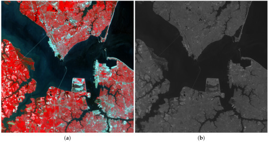
Figure 1. Observed LANDSAT 7-ETM+ Chesapeake Bay image: (a) $1024\times 1024$ multispectral (MS), (b) $2048\times 2048$ panchromatic (PAN).

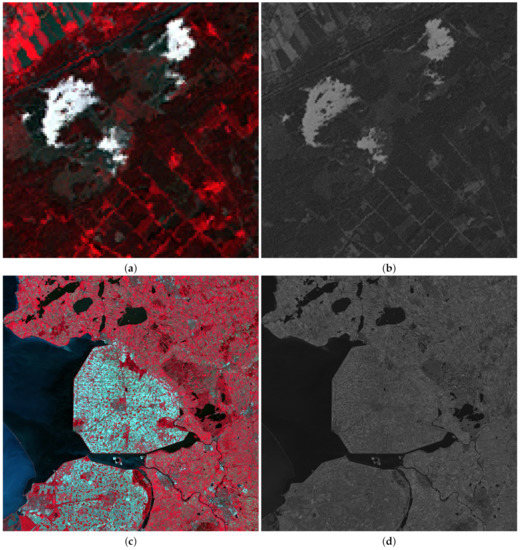
Figure 2. Observed LANDSAT 7-ETM+ Netherland images: (a) $128\times 128$ MS, (b) $256\times 256$ PAN, (c) $2048\times 2048$ MS, (d) $4096\times 4096$ PAN.

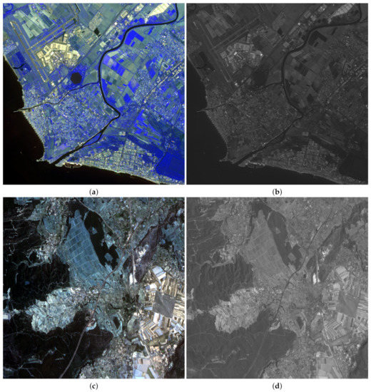
Figure 3. Observed SPOT-5 Roma image: (a) $1024\times 1024$ MS, (b) $4096\times 4096$ PAN. FORMOSAT-2 Salon-de-Provence image: (c) $1024\times 1024$ MS, (d) $4096\times 4096$ PAN.

Both the observed $\mathbf{Y}$ and $\mathbf{x}$ images have been normalized to the range $[0,1]$ before running Algorithm 1. The convergence criterion in the algorithm was $\Vert {⟨\mathbf{y}⟩}^{(n)}-{⟨\mathbf{y}⟩}^{(n-1)}{\Vert }^2/{\Vert {⟨\mathbf{y}⟩}^{(n)}\Vert }^2\le {10}^{-6}$ or 50 iterations were reached, whatever occurs first. The relationship between the MS high resolution image and the panchromatic image in Equation (2) is governed by the parameters $\mathit{\lambda }$ that need to be set before pansharpening is carried out. If we knew the sensor spectral response characteristics, the values of $\mathit{\lambda }$ could be estimated from them. For instance, for LANDSAT 7-ETM+, Figure 4 shows the sensor spectral response curves for the MS bands B1-B6, shown in color, and the PAN band shown in black. For this sensor, the PAN band mainly overlaps B2-B4 MS bands, and $\mathit{\lambda }$ coefficients could be obtained from this overlapping (see [52]). In this paper, however, a more general approach is followed to estimate $\mathit{\lambda }$ from the observations. First, we define $\mathbf{X}=\mathbf{D}\mathbf{x}$, a version of the PAN image downsampled to the size of the MS image. Then, since the sensor spectral response is the same in high and low resolution, the parameters $\mathit{\lambda }$ can be obtained by solving

$$\begin{array}{cc}\hfill & \lambda =\underset{\lambda }{argmin}{\Vert \mathbf{X}-\sum _{b=1}^B{\lambda }_b{\mathbf{Y}}_b\Vert }^2,\hfill \end{array}$$

(29)

$$\begin{array}{cc}\hfill & \mathrm{subject} \mathrm{sto}{\lambda }_b\ge 0,\forall b,\sum _{b=1}^B{\lambda }_b=1.\hfill \end{array}$$

(30)

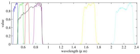
Figure 4. LANDSAT 7-ETM+ band spectral response normalized to one.

Table 2 shows the $\lambda s$ associated to the different considered observed images. For the LANDSAT 7-ETM+ images only the first four bands are positive and ${\lambda }_5$ and ${\lambda }_6$ values are 0 since we know that bands B5 and B6 are not covered by the panchromatic sensor. For this process, each band is normalized to the interval $[0,1]$. Note that due to the normalization, the estimated $\lambda$ values do not only depend on the sensor spectral response but also on the observed area characteristics. This explains the differences between the obtained $\lambda$ values for the images in Figure 2a,c. Although those images are from the same area of Netherlands, clouds in Figure 2a modify the estimation of the values of $\lambda$.

Table 2. Estimated $\mathit{\lambda }$ values for the different sensors.

Sensor	Image	B1	B2	B3	B4	B5	B6
LANDSAT 7-ETM+	Figure 1	0.0986	0.1011	0.2576	0.5427	0	0
LANDSAT 7-ETM+	Figure 2a	0.0183	0.4243	0.0576	0.4998	0	0
LANDSAT 7-ETM+	Figure 2c	0	0.2283	0.1611	0.6106	0	0
SPOT-5	Figure 3a	0	0.2993	0.6897	0.0110	-	-
FORMOSAT-2	Figure 3c	0.0384	0.5566	0	0.4051	-	-

6. Discussion

Within the variational Bayesian methodology, two methods are proposed in this paper: one using the log penalty function (see Table 1), hence, named log method, and another using the ${\ell }_p$ penalty function, with $p=1$, referred as $\ell 1$ method. The proposed methods have been compared with the following classic and state-of-the-art pansharpening methods: the Principal Component Analysis (PCA) [6], the Intensity–Hue–Saturation (IHS) transform [19], the Brovey transform (Brovey) [7], the Band-Dependent Spatial-Detail (BDSD) method in [22], the Gram-Schmidt (GS) method in [20], the Gram-Schmidt adaptive (GSA) method in [21], the Partial Replacement Adaptive Component Substitution (PRACS) method in [23], the High Pass Filtering (HPF) algorithm in [18], the Smoothing Filter Based Intensity Modulation (SFIM) method [35,36], the Indusion method in [37], the Additive A Trous Wavelet Transform (ATWT) in [26], the Additive Wavelet Luminance Proportional (AWLP) method in [28], the ATWT Model 2 (ATWT-M2) and ATWT Model 3 (ATWT-M3) methods in [10], the Generalized Laplacian Pyramid (GLP)-based methods in [29], concretely the modulation transfer functions (MTF)-GLP, GLP with High Pass Modulation (MTF-GLP-HPM), and GLP with Context Based Decision (MTF-GLP-CBD) methods, and the pansharpening method using a Total Variation (TV) image model in [53]. We have used the implementation of the methods and measures provided by the Pansharpening Toolbox (https://rscl-grss.org/coderecord.php?id=541) [13]. For those methods not included in the toolbox we have used the code provided by the authors. The code of the proposed methods will be publicly available at https://github.com/vipgugr. We have also included the results of bilinear interpolating the MS image to the size of the PAN, marked as EXP, as a reference. Both quantitative and qualitative comparisons of the different methods have been performed.

6.1. Quantitative Comparison

A common problem in pansharpening is the nonexistence of a MS high resolution ground-truth image to compare with. Hence we performed two kinds of quantitative comparisons. Firstly, the images obtained using the different methods have been compared following Wald’s protocol [73] as follows: the observed MS image, $\mathbf{Y}$, and the PAN image, $\mathbf{x}$, are downsampled by applying the operator $\mathbf{D}$ to generate low resolution versions of them. Then, pansharpening is applied to those low resolution images and the obtained estimation of the MS image, $\widehat{\mathbf{y}}$, is quantitatively compared with the observed MS image, $\mathbf{Y}$. Secondly, the different methods have been compared using Quality with No Reference (QNR) measures [13,74]. As previously stated, for the LANDSAT image in Figure 1, the resolution ratio between MS and PAN images is $p/P=4$. Since the SPOT-5 satellite provides two PAN images, two experiments were carried out on the image in Figure 3, one with a decimation ratio of 4 and another with a ratio of 16. For the FORMOSAT-2 image the ratio is $p/P=16$. However, for the sake of completeness, two experiments were also carried out, one assuming a decimation ratio of 4 and another with a ratio of 16.

Both spatial and spectral quality metrics have been used to compare the results obtained using the different methods. Details for the metrics used is shown below:

Spatial measures:

• Q

  –

  Universal Quality Index (UQI) [75] averaged on all MS bands.

  –

  Range: [-1, 1]

  –

  The higher the the better.

• Q4, Q8

  –

  Instances of the $Q{2}^n$ [76] index taking values. Suitable to measure quality for multiband images having an arbitrary number of spectral bands. Q4 is used for SPOT-5 and FORMOSAT-2 images which have four bands and Q8 for the LANDSAT image with six bands.

  –

  Range: [0, 1]

  –

  The higher the better.

• Spatial Correlation Coefficient (SCC) [77]

  –

  Measures the correlation coefficient between compared images after the application of a Sobel filter.

  –

  Range: [0, 1]

  –

  The higher the better.

• QNR spatial distortion ($D_S$) [78]

  –

  Measures the spatial distortion between MS bands and PAN image.

  –

  Range: [0, 1]

  –

  The lower the better.

Spectral measures:

• Spectral Angle Mapper (SAM) [79]

  –

  For spectral fidelity. Measures the mean angle between the corresponding pixels of the compared images in the space defined by considering each spectral band as a coordinate axis

  –

  Range: [0, 180]

  –

  The lower the better.

• Erreur Relative Globale Adimensionnelle de Synthese (ERGAS) [80]

  –

  Measures spectral consistency between compared images.

  –

  Range: $[0,\infty [$

  –

  The lower ERGAS value the better consistency, specially for values lower than the number of image bands B.

• QNR spectral distortion ($D_{\lambda }$) [78]

  –

  This measure is derived from the differences between the inter-band Q index values computed for HR and LR images.

  –

  Range: [0, 1]

  –

  The lower, the better.

Spatial and spectral measures:

• Jointly Spectral and Spatial Quality Index (QNR) [78]

  –

  QNR is obtained as the product of (1-$D_S$) and (1-$D_{\lambda }$).

  –

  Range: [0, 1]

  –

  The higher the better.

Table 3 shows the obtained figures of merit using Wald’s protocol for the LANDSAT image in Figure 1. As it is clear from the table, ℓ1 outperforms all the other methods both in spectral fidelity and the incorporation of spatial details. Note the high SCC value (meaning that the details in the PAN image have been successfully incorporated into the pansharpened image) while also obtaining the lowest spectral distortion as evidenced by the SAM and ERGAS values. The TV method obtains the second best results except for the SAM metric, for this metric, the proposed log method has the second best value. This method also obtains the third best values for ERGAS and SCC measures. GLP based and PRACS methods also obtain high values for the Q, Q8 indices and low value for SAM. However, their ERGAS and SCC performance is worse. Table 4 shows the QNR quantitative results for the LANDSAT image in Figure 1. In this table, the proposed methods achieve competitive results. Log obtains the best $D_{\lambda }$ value and this method together with ℓ1 obtain second and third QNR scores, respectively. Note that EXP obtained the highest score using QNR since bilinear interpolation of the observed MS low resolution image is used as the MS high resolution estimation to calculate $D_S$ and $D_{\lambda }$ calculations.

Table 3. Quantitative results on the LANDSAT 7-ETM+ Chesapeake Bay image. Bold values indicate the best score.

Method	Q8	Q	SAM	ERGAS	SCC
EXP	0.8335	0.8383	2.0223	5.1113	0.8718
PCA	0.7830	0.8074	2.7937	5.8086	0.8569
IHS	0.6795	0.6734	2.6640	7.8586	0.8223
Brovey	0.6798	0.6790	2.1605	7.5226	0.8148
BDSD	0.7599	0.7829	2.4662	5.9244	0.8539
GS	0.7447	0.7401	3.3052	8.7258	0.8040
GSA	0.8010	0.8202	2.4033	5.0688	0.8764
PRACS	0.8363	0.8423	2.0998	4.8655	0.8774
HPF	0.8137	0.8243	2.2221	5.1279	0.8834
SFIM	0.8008	0.8184	2.1857	5.0228	0.8905
Indusion	0.8052	0.8167	2.2906	5.5412	0.8495
ATWT	0.8100	0.8208	2.3482	5.3642	0.8809
AWLP	0.8267	0.8315	2.2516	5.3873	0.8734
ATWT-M2	0.7737	0.7802	2.6004	5.8133	0.8317
ATWT-M3	0.7884	0.7925	2.5720	5.8973	0.8367
MTF-GLP	0.8157	0.8258	2.2418	5.1307	0.8838
MTF-GLP-HPM	0.8037	0.8206	2.1878	5.0236	0.8918
MTF-GLP-CBD	0.8200	0.8292	2.2499	5.1015	0.8809
TV	0.8492	0.8606	2.1362	4.2505	0.9163
$\ell \mathbf{1}$	0.8595	0.8694	1.8518	4.0954	0.9220
log	0.7951	0.7856	1.8839	4.4819	0.9007

Table 4. QNR Quantitative results on the LANDSAT 7-ETM+ Chesapeake Bay image. Bold values indicate the best score.

	${\mathit{D}}_{\lambda }$	${\mathit{D}}_{\mathit{S}}$	QNR
EXP	0.0096	0.0166	0.9740
PCA	0.0555	0.1459	0.8066
IHS	0.1049	0.2888	0.6366
Brovey	0.0963	0.2290	0.6968
BDSD	0.1055	0.1486	0.7616
GS	0.0716	0.1992	0.7435
GSA	0.0605	0.1167	0.8298
PRACS	0.0154	0.0823	0.9035
HPF	0.0857	0.1308	0.7947
SFIM	0.0834	0.1146	0.8116
Indusion	0.0595	0.0525	0.8911
ATWT	0.1044	0.1500	0.7612
AWLP	0.1045	0.1517	0.7596
ATWT-M2	0.1530	0.2327	0.6499
ATWT-M3	0.1227	0.1975	0.7041
MTF-GLP	0.0917	0.1378	0.7831
MTF-GLP-HPM	0.0890	0.1215	0.8004
MTF-GLP-CBD	0.0585	0.1081	0.8397
TV	0.0425	0.0919	0.8695
l1	0.0338	0.0527	0.9153
log	0.0090	0.0364	0.9549

Table 5 and Table 6 show the quantitative results using Wald’s protocol for the LANDSAT images in Figure 2a,c, respectively. PRACS outperforms all other methods on the image in Figure 2a (see Table 5) and the proposed ℓ1 and log obtain the first and second best scores on the image in Figure 2c (see Table 6). Table 7 and Table 8 show the obtained QNR figures of merit for those two images. The proposed methods produce good $D_S$, $D_{\lambda }$ and QNR values for both images, both above 0.9 which supports their good performance. Again the EXP results are the best in all the measures for Table 8 and provides the best $D_{\lambda }$, for the image associated to Table 7. The ℓ1 method obtains the best $D_S$ for this image and BDSD the highest QNR.

Table 5. Quantitative results using Wald’s protocol on the LANDSAT 7-ETM+ Netherland image in Figure 2a. Bold values indicate the best score.

	Q8	Q	SAM	ERGAS	SCC
EXP	0.4727	0.8849	3.0445	7.7235	0.8686
PCA	0.3759	0.7617	3.8165	12.6420	0.8205
IHS	0.3322	0.7479	1.7633	10.7598	0.8570
Brovey	0.2892	0.7675	0.0000	10.7809	0.8492
BDSD	0.7205	0.9520	1.7296	4.6748	0.9777
GS	0.3860	0.7833	3.3486	11.7850	0.8323
GSA	0.5543	0.8474	2.5086	10.2990	0.8707
PRACS	0.8230	0.9720	0.9558	2.9097	0.9878
HPF	0.6420	0.9045	2.0699	7.4387	0.9458
SFIM	0.5950	0.9043	1.8898	8.1778	0.9379
Indusion	0.4108	0.8406	3.6963	9.6521	0.8269
ATWT	0.5582	0.8741	2.6859	9.6507	0.9267
AWLP	0.4715	0.8741	2.2059	10.1057	0.9195
ATWT-M2	0.3943	0.8436	3.7879	8.7289	0.8606
ATWT-M3	0.4861	0.8685	3.5274	7.7506	0.8829
MTF-GLP	0.5975	0.8946	2.2544	8.1279	0.9351
MTF-GLP-HPM	0.5659	0.8926	2.0133	9.0221	0.9272
MTF-GLP-CBD	0.6095	0.9001	2.1726	7.8290	0.9392
TV	0.4798	0.8906	3.4873	7.1207	0.8977
l1	0.4815	0.9044	3.3783	6.9422	0.9022
log	0.4931	0.8920	2.9187	6.9321	0.8952

Table 6. Quantitative results using Wald’s protocol on the LANDSAT 7-ETM+ Netherland image in Figure 2c. Bold values indicate the best score.

	Q8	Q	SAM	ERGAS	SCC
EXP	0.7874	0.7867	3.3362	5.9279	0.8521
PCA	0.6167	0.4854	5.7078	12.8127	0.5788
IHS	0.5343	0.3778	4.7417	12.9526	0.5918
Brovey	0.5465	0.4063	3.4605	13.0876	0.5960
BDSD	0.7575	0.7733	3.9348	6.8610	0.7856
GS	0.5899	0.4369	6.1158	13.9275	0.5522
GSA	0.7323	0.7444	4.0920	7.2078	0.7535
PRACS	0.7822	0.7829	3.4787	6.3244	0.8037
HPF	0.7167	0.7241	3.8135	7.3266	0.7603
SFIM	0.6908	0.7181	4.6693	9.0262	0.7261
Indusion	0.7230	0.7346	3.8229	7.2177	0.7631
ATWT	0.6948	0.6971	4.0402	8.0306	0.7240
AWLP	0.7110	0.7066	3.8124	8.1733	0.7165
ATWT-M2	0.6332	0.6288	4.5223	8.5542	0.6135
ATWT-M3	0.6993	0.6967	4.3028	7.4420	0.7201
MTF-GLP	0.7116	0.7172	3.8632	7.5134	0.7457
MTF-GLP-HPM	0.6875	0.7133	4.6780	9.1110	0.7161
MTF-GLP-CBD	0.7519	0.7595	3.7522	6.8698	0.7740
TV	0.7843	0.8065	3.8402	5.7351	0.8519
l1	0.8118	0.8196	3.1337	5.1831	0.8853
log	0.7750	0.7682	3.0810	5.3115	0.8818

Table 7. QNR quantitative results on the LANDSAT 7-ETM+ Netherland image in Figure 2a. Bold values indicate the best score.

	${\mathit{D}}_{\lambda }$	${\mathit{D}}_{\mathit{S}}$	QNR
EXP	0.0104	0.0593	0.9309
PCA	0.2463	0.3998	0.4523
IHS	0.2632	0.4035	0.4394
Brovey	0.2182	0.3873	0.4790
BDSD	0.0159	0.0505	0.9344
GS	0.2335	0.4067	0.4548
GSA	0.2139	0.3240	0.5314
PRACS	0.0665	0.2106	0.7369
HPF	0.1711	0.2638	0.6102
SFIM	0.1610	0.2513	0.6282
Indusion	0.1354	0.1612	0.7252
ATWT	0.1968	0.2961	0.5654
AWLP	0.1977	0.2954	0.5653
ATWT-M2	0.1727	0.3127	0.5686
ATWT-M3	0.1187	0.2143	0.6924
MTF-GLP	0.1796	0.2791	0.5915
MTF-GLP-HPM	0.1688	0.2661	0.6100
MTF-GLP-CBD	0.1741	0.2778	0.5965
TV	0.0912	0.1127	0.8064
l1	0.0342	0.0386	0.9286
log	0.0157	0.0627	0.9225

Table 8. QNR quantitative results on the LANDSAT 7-ETM+ Netherland image in Figure 2c. Bold values indicate the best score.

	${\mathit{D}}_{\lambda }$	${\mathit{D}}_{\mathit{S}}$	QNR
EXP	0.0067	0.0157	0.9778
PCA	0.1893	0.5019	0.4038
IHS	0.2040	0.5973	0.3205
Brovey	0.1979	0.5227	0.3829
BDSD	0.0134	0.0107	0.9761
GS	0.1999	0.5237	0.3811
GSA	0.0986	0.2337	0.6907
PRACS	0.0255	0.1176	0.8599
HPF	0.1594	0.2772	0.6075
SFIM	0.1124	0.2272	0.6859
Indusion	0.1352	0.2054	0.6871
ATWT	0.1822	0.3234	0.5534
AWLP	0.1765	0.3101	0.5682
ATWT-M2	0.1903	0.3467	0.5290
ATWT-M3	0.0917	0.1581	0.7647
MTF-GLP	0.1656	0.2933	0.5897
MTF-GLP-HPM	0.1164	0.2424	0.6694
MTF-GLP-CBD	0.0854	0.1953	0.7359
TV	0.0381	0.1186	0.8478
l1	0.0228	0.0704	0.9084
log	0.0073	0.0199	0.9730

Figure 5 and Figure 6 show a zoomed in region of the RGB color images formed by bands B4, B3, and B2 of MS ground truth images used to apply Wald’s protocol and also the absolute error images for the methods in Table 7 and Table 8. In those images, the darker the intensity the lower the absolute error. Figure 5 and Figure 6 are consistent with the quantitative comparison shown in Table 5 and Table 6, respectively. The best results for the image in Figure 2a were obtained using PRACS, while for the image in Figure 2c the best performing method is ℓ1. Note that brighter areas in Figure 5e,f correspond to the borders of cloudy areas in Figure 2a. We argue that since clouds alter the weights of $\mathit{\lambda }$ estimated using Equation (30), the boundaries of clouds and land areas in Figure 2a are not well resolved. This explains a worse behavior of the proposed methods in the cloudy areas of this image.

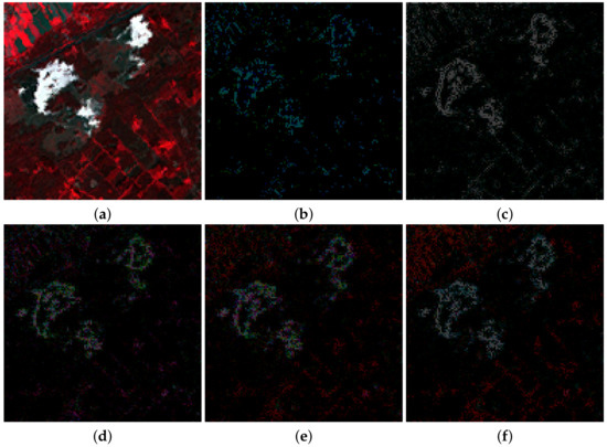
Figure 5. (a) Ground truth $128\times 128$ image from Figure 2a. The normalized maximum absolute error minus the absolute error images images for the following methods, (b) Partial Replacement Adaptive Component Substitution (PRACS), (c) modulation transfer functions (MTF)-generalized Laplacian pyramid (GLP)-context based decision (CBD), (d) Total Variation (TV), (e) ℓ1 and (f) log.

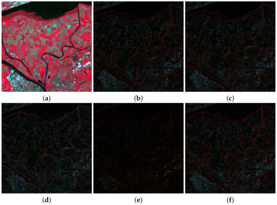
Figure 6. (a) Ground truth $256\times 256$ image from Figure 2c. The normalized maximum absolute error images for the following methods: (b) PRACS, (c) MTF-GLP-CBD, (d) TV, (e) ℓ1 and (f) log.

Table 9 and Table 10 show, respectively, the quantitative results using Wald’s protocol for the SPOT-5 and the FORMOSAT-2 images in Figure 3 for the decimation ratios $p/P=4$ and $p/P=16$. The proposed log obtains the best figures of merit for the SPOT image in Figure 3a with $p/P=4$ except for Q and Q4 metrics. The Q values obtained by log and ℓ1 are slightly lower than those obtained by BDSD. Note that BDSD achieved the third best general figures just below the proposed log and ℓ1 algorithms. With $p/P=16$ the proposed log algorithm provides the best results except for Q, Q4 and SAM values, where competitive values are obtained. The proposed log achieves a slightly lower Q value than PRACS and a slightly higher SAM value than Brovey. In general, PRACS is the second best performing method for this image for $p/P=16$. For the FORMOSAT-2 image in Figure 3c, the proposed ℓ1 and log algorithms obtained the best numerical results for a $p/P=4$ magnification. Both methods provide similar results, which are better than all the one provided by the competing methods. For a ratio $p/P=16$, there is not a clear winner. The proposed methods are competitive in this image although they do not stand out in any of the measures. Table 11 and Table 12 show, respectively, the QNR quantitative results for the SPOT-5 and the FORMOSAT-2 images in Figure 3 for the decimation ratios $p/P=4$ and $p/P=16$. In Table 11, EXP achieves the best $D_S$, $D_{\lambda }$ and QNR scores. In this table, the proposed methods obtain good scores. The log method obtains the second best $D_{\lambda }$ and $D_S$ values and very high QNR values for both decimation ratios. Results for the FORMOSAT image, shown in Table 12, are very similar although in this case, BDSD obtains the best $D_S$ and QNR values for $p/P=4$ and ATWT-M3 for $p/P=16$.

Table 9. Quantitative results using Wald’s protocol on the SPOT-5 Roma image. Bold values indicate the best score.

$\mathit{p}/\mathit{P}$	4					16
Method	Q4	Q	SAM	ERGAS	SCC	Q4	Q	SAM	ERGAS	SCC
EXP	0.8766	0.8859	1.7048	3.7857	0.8640	0.7325	0.7407	2.5071	2.8441	0.6049
PCA	0.4067	0.5360	5.1646	12.3346	0.2788	0.3927	0.5091	5.7208	6.2911	0.2443
IHS	0.4072	0.5238	3.9951	12.2342	0.2772	0.3973	0.5051	4.4508	6.1770	0.2520
Brovey	0.4124	0.5337	1.8413	12.1960	0.2594	0.4019	0.5124	2.4000	6.1718	0.2482
BDSD	0.8559	0.8825	2.0565	4.2776	0.8235	0.5947	0.6231	3.0328	4.3050	0.2804
GS	0.4102	0.5364	5.0523	12.1272	0.2634	0.3985	0.5124	5.5849	6.1471	0.2405
GSA	0.4897	0.5384	2.9893	11.0363	0.1932	0.4997	0.5354	3.1189	5.3703	0.2164
PRACS	0.8220	0.8380	2.0536	4.8936	0.7298	0.7291	0.7458	2.5190	2.9647	0.5295
HPF	0.7488	0.7695	2.0632	6.3388	0.6250	0.5888	0.6124	2.8370	4.5969	0.2988
SFIM	0.7744	0.7860	1.9658	6.0694	0.6447	0.6052	0.6232	2.6792	4.4425	0.3079
Indusion	0.7473	0.7894	2.1609	5.9717	0.6761	0.5301	0.5935	3.5689	4.9656	0.3408
ATWT	0.6928	0.7171	2.2358	7.6433	0.5183	0.5849	0.6092	2.8932	4.7245	0.3099
AWLP	0.7066	0.7260	2.1798	7.6246	0.5075	0.5947	0.6173	2.8504	4.6963	0.3052
ATWT-M2	0.7229	0.7343	2.3084	6.3145	0.4678	0.6723	0.6822	2.7291	3.3277	0.3965
ATWT-M3	0.7837	0.7930	2.2394	5.1935	0.6714	0.6924	0.7019	2.7026	3.1094	0.4801
MTF-GLP	0.7289	0.7507	2.1201	6.7975	0.5766	0.5775	0.6023	2.9275	4.8355	0.3022
MTF-GLP-HPM	0.7553	0.7675	2.0005	6.4923	0.5972	0.5928	0.6111	2.7388	4.7066	0.3073
MTF-GLP-CBD	0.7718	0.7870	2.0188	6.0490	0.6215	0.6021	0.6217	2.7767	4.5632	0.3118
TV	0.7472	0.7893	3.1882	6.1393	0.6162	0.6480	0.6872	3.5109	3.9763	0.3265
$\ell \mathbf{1}$	0.8617	0.8783	2.0688	4.1557	0.8196	0.6409	0.7017	3.7793	3.7117	0.3792
log	0.8636	0.8762	1.6053	3.3673	0.8923	0.7323	0.7395	2.4228	2.7072	0.6262

Table 10. Quantitative results using Wald’s protocol on the FORMOSAT-2 Salon-de-Provence image. Bold values indicate the best score.

$\mathit{p}/\mathit{P}$	4					16
Method	Q4	Q	SAM	ERGAS	SCC	Q4	Q	SAM	ERGAS	SCC
EXP	0.8610	0.8617	1.8158	3.7257	0.8460	0.6918	0.6925	2.5057	2.6934	0.5906
PCA	0.7858	0.8089	2.2098	5.0711	0.6595	0.7415	0.7668	2.6373	2.7485	0.5870
IHS	0.7912	0.8159	1.9637	4.6293	0.6695	0.7445	0.7720	2.4527	2.5803	0.5894
Brovey	0.7861	0.8146	1.9106	4.5332	0.6644	0.7385	0.7687	2.4345	2.5597	0.5793
BDSD	0.8443	0.8545	2.0292	4.2608	0.7232	0.7701	0.7823	2.5460	2.7217	0.5821
GS	0.7979	0.8195	2.1375	4.9193	0.6619	0.7506	0.7753	2.5761	2.6860	0.5888
GSA	0.7859	0.8167	2.1855	5.2508	0.6508	0.7607	0.7772	2.5510	2.7698	0.5796
PRACS	0.8495	0.8592	1.9581	4.0842	0.7373	0.7947	0.8016	2.4240	2.3683	0.6230
HPF	0.8469	0.8523	1.9799	4.2210	0.7782	0.7813	0.7885	2.4609	2.5388	0.5900
SFIM	0.8470	0.8523	1.9821	4.2718	0.7755	0.7817	0.7888	2.4600	2.5658	0.5874
Indusion	0.8304	0.8371	2.0075	4.4361	0.7407	0.7519	0.7698	2.4986	2.6941	0.5758
ATWT	0.8391	0.8449	2.0374	4.5675	0.7663	0.7901	0.7965	2.4679	2.5399	0.6161
AWLP	0.8408	0.8473	1.8896	4.3549	0.7671	0.7909	0.7979	2.3689	2.4540	0.6150
ATWT-M2	0.8277	0.8326	2.2307	4.2164	0.6975	0.7672	0.7704	2.5499	2.3709	0.6325
ATWT-M3	0.8325	0.8356	2.2137	4.0586	0.7341	0.7639	0.7660	2.5659	2.3878	0.6384
MTF-GLP	0.8477	0.8533	1.9883	4.2705	0.7704	0.7901	0.7968	2.4714	2.5563	0.6176
MTF-GLP-HPM	0.8476	0.8532	1.9889	4.3313	0.7676	0.7904	0.7971	2.4666	2.5937	0.6158
MTF-GLP-CBD	0.8493	0.8548	2.0076	4.2575	0.7730	0.7846	0.7916	2.5270	2.6394	0.6123
TV	0.8696	0.8790	2.1437	3.7602	0.7876	0.7807	0.7878	2.7906	2.4374	0.5956
$\ell \mathbf{1}$	0.8946	0.8974	1.9200	3.3526	0.8457	0.7691	0.7625	3.0726	2.6041	0.5503
log	0.8706	0.8683	1.7597	3.3686	0.8751	0.6889	0.6848	2.4975	2.6009	0.6050

Table 11. QNR Quantitative results on the SPOT-5 Roma image. Bold values indicate the best score.

$\mathit{p}/\mathit{P}$	4			16
	${\mathbf{D}}_{\mathbf{\lambda }}$	${\mathbf{D}}_{\mathbf{S}}$	QNR	${\mathbf{D}}_{\mathbf{\lambda }}$	${\mathbf{D}}_{\mathbf{S}}$	QNR
EXP	0.0041	0.0150	0.9809	0.0001	0.0312	0.9687
PCA	0.2047	0.4094	0.4697	0.3094	0.5035	0.3429
IHS	0.2389	0.4158	0.4447	0.3574	0.5143	0.3121
Brovey	0.1804	0.3799	0.5082	0.2890	0.4754	0.3730
BDSD	0.0108	0.0922	0.8980	0.0388	0.0344	0.9281
GS	0.1964	0.4100	0.4741	0.3045	0.5044	0.3447
GSA	0.2194	0.3421	0.5135	0.3267	0.4287	0.3846
PRACS	0.0325	0.1555	0.8171	0.0656	0.2162	0.7324
HPF	0.0851	0.1405	0.7864	0.2149	0.2556	0.5844
SFIM	0.0661	0.1256	0.8167	0.1949	0.2416	0.6107
Indusion	0.0580	0.0370	0.9072	0.2458	0.1587	0.6345
ATWT	0.1310	0.2119	0.6849	0.2398	0.3037	0.5293
AWLP	0.1030	0.1950	0.7221	0.2015	0.2814	0.5738
ATWT-M2	0.0728	0.2002	0.7416	0.0996	0.1691	0.7482
ATWT-M3	0.0162	0.0349	0.9494	0.0493	0.0328	0.9195
MTF-GLP	0.1040	0.1586	0.7539	0.2511	0.3000	0.5242
MTF-GLP-HPM	0.0858	0.1441	0.7825	0.2314	0.2868	0.5481
MTF-GLP-CBD	0.0657	0.1272	0.8154	0.1922	0.2681	0.5912
TV	0.3399	0.1830	0.5394	0.1866	0.1510	0.6906
l1	0.0277	0.0378	0.9356	0.1927	0.1500	0.6862
log	0.0056	0.0272	0.9674	0.0422	0.0380	0.9214

Table 12. QNR quantitative results on the FORMOSAT-2 Salon-de-Provence image. Bold values indicate the best score.

$\mathit{p}/\mathit{P}$	4			16
	${\mathbf{D}}_{\mathbf{\lambda }}$	${\mathbf{D}}_{\mathbf{S}}$	QNR	${\mathbf{D}}_{\mathbf{\lambda }}$	${\mathbf{D}}_{\mathbf{S}}$	QNR
EXP	0.0087	0.0837	0.9083	0.0086	0.0931	0.8990
PCA	0.1108	0.2190	0.6945	0.1503	0.3083	0.5877
IHS	0.1083	0.2127	0.7020	0.1508	0.3027	0.5921
Brovey	0.0859	0.1964	0.7345	0.1215	0.2815	0.6312
BDSD	0.0179	0.0150	0.9673	0.0264	0.1775	0.8008
GS	0.0970	0.2084	0.7149	0.1366	0.2971	0.6069
GSA	0.1254	0.2095	0.6914	0.1618	0.2963	0.5899
PRACS	0.0621	0.1656	0.7826	0.0878	0.2413	0.6921
HPF	0.0896	0.1130	0.8075	0.1147	0.1559	0.7473
SFIM	0.0877	0.1121	0.8101	0.1128	0.1556	0.7492
Indusion	0.0510	0.0174	0.9325	0.0938	0.0965	0.8187
ATWT	0.1227	0.1529	0.7432	0.1355	0.1951	0.6958
AWLP	0.1290	0.1500	0.7404	0.1393	0.1887	0.6983
ATWT-M2	0.1184	0.1550	0.7449	0.0967	0.1238	0.7915
ATWT-M3	0.0871	0.0951	0.8261	0.0586	0.0388	0.9049
MTF-GLP	0.1004	0.1277	0.7847	0.1437	0.1996	0.6854
MTF-GLP-HPM	0.0980	0.1269	0.7875	0.1410	0.1989	0.6881
MTF-GLP-CBD	0.0910	0.1222	0.7979	0.1317	0.1919	0.7017
TV	0.1114	0.0787	0.8186	0.0951	0.1811	0.7410
l1	0.0425	0.0514	0.9083	0.0594	0.0847	0.8609
log	0.0094	0.0917	0.8998	0.0174	0.1011	0.8832

Table 13 shows the required CPU time in seconds on a 2.40GHz Intel^® Xeon^® CPU for the pansharpening of a MS image with 4 bands to a $1024\times 1024$ size, for $p/P=4$ and $p/P=16$, using the different methods under comparison. Equation (18) has been solved using the Conjugate Gradient method which required, to achieve convergence, less than 30 iterations for the ℓ1 prior and at least 1000 iterations for the log prior. This explains the differences between their required CPU time. Note that the proposed methods automatically estimate the model parameters which increases the running time but makes our methods parameter free.

Table 13. Elapsed CPU time in seconds for the different pansharpening methods on a 1024 × 1024 image and with different $p/P$ ratios.

P	p	PCA	IHS	Brovey	BDSD	GS
$512\times 512$	$1024\times 1024$	0.9	0.04	0.04	0.9	0.4
$256\times 256$	$1024\times 1024$	0.3	0.03	0.03	0.8	0.3
P	p	GSA	PRACS	HPF	SFIM	Indusion
$512\times 512$	$1024\times 1024$	1	2.2	0.2	0.5	0.5
$256\times 256$	$1024\times 1024$	1.6	1.2	0.2	0.18	0.3
P	p	ATWT	AWLP	ATWT-M2	ATWT-M3	MTF-GLP
$512\times 512$	$1024\times 1024$	11	14	10	10	0.9
$256\times 256$	$1024\times 1024$	3	3	7	7	0.6
P	p	MTF-HPM	MTF-CBD	TV	ℓ1	log
$512\times 512$	$1024\times 1024$	0.8	2	1.5 ${10}^3$	808	1.1 ${10}^4$
$256\times 256$	$1024\times 1024$	0.6	0.6	1.6 ${10}^3$	3 ${10}^3$	2.8 ${10}^4$

6.2. Qualitative Comparison

Figure 7 shows a small region of interest of the observed LANDSAT-7 images in Figure 1 and the pansharpening results with $p/P=4$ obtained by the proposed methods and the competing ones with the best quantitative performance, that is, PRACS, MTF-GLP-HPM, MTF-GLP-CBD and TV methods. All color images in this figure are RGB images formed from the B4, B3 and B2 Landsat bands. Since we are using full resolution images, there is no ground truth to compare with, so a visual analysis of the resulting images is performed. The improved resolution of all the pansharpening results in Figure 7c–h with respect to the observed MS image in Figure 7a is evident. PRACS, MTF-GLP-HPM and MTF-GLP-CBD images in Figure 7c–e have a lower detail level than TV and the proposed ℓ1 method, see Figure 7f,g, respectively. See, for instance, the staircase effects in some diagonal edges not present in the TV and proposed ℓ1 method results. The PRACS, MTF-GLP-HPM and MTF-GLP-CBD methods produce similar, but lower, spectral quality than the proposed method, which is consistent with the numerical results in Table 3 and discussion presented in Section 6.1. The image obtained using the ℓ1 method, Figure 7g, has colors closer to those of the observed MS image than the TV image, Figure 7f, which is also somewhat noisier. The log method is very good at removing noise in the image (see the sea area) but it tends to remove other fine details too.

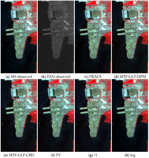
Figure 7. A region of interest of the LANDSAT 7-ETM+ Chesapeake Bay image in Figure 1a. Observed images: (a) $128\times 64$ MS, (b) $256\times 128$ PAN. $256\times 128$ pansharpened images by: (c) PRACS, (d) MTF-GLP-High Pass Modulation (HPM), (e) MTF-GLP-CBD, (f) TV, (g) ℓ1 and (h) log methods.

Figure 8 shows a region of interest of the observed SPOT-5 images in Figure 3a,b and the pansharpening results with $p/P=16$ obtained using the competing methods with the best performance on this image, that is, Brovey, PRACS, ATWT-M3, and TV methods, and the proposed ℓ1 and log methods. All color images in this figure are RGB images formed from the bands B3, B2 and B1 of the SPOT-5 image. The Brovey method (Figure 8c) produces the highest spectral distortion, however, it also recovers more spatial details in the image (see the airport runway and plane). ATWT-M3 (Figure 8e), on the other hand, produces a blurry image. PRACS produces a sharper image, see Figure 8d, but details in the PAN image do not seem to be well-integrated. The TV method (Figure 8f) and the proposed ℓ1 and log methods (Figure 8g,h obtain the most consistent results, with high spatial details and low spectral distortion. However, TV introduces staircase artifacts on diagonal lines that are not noticeable in the ℓ1 and log images. As with the LANDSAT-7 image, the log image in Figure 8h lacks some small details, removed by the method along with noise.

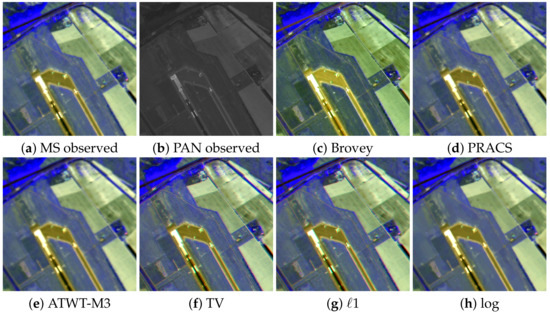
Figure 8. A region of interest of the SPOT-5 Roma image in Figure 3a. Observed images: (a) $128\times 128$ MS, (b) $512\times 512$ PAN. $512\times 512$ pansharpened images by: (c) Brovey, (d) PRACS, (e) Additive A Trous Wavelet Transform (ATWT)-M3, (f) TV, (g) ℓ1 and (h) log methods.

7. Conclusions

A variational Bayesian methodology for the pansharpening problem has been proposed. In this methodology, we model the relation between the MS high resolution image and the PAN image as a linear combination of the MS bands whose weights are estimated from the available data. The observed MS image is modelled as a downsampled version of the original MS image. The expected characteristics of the pansharpened image are incorporated in the form of SG sparse image priors. Two penalty functions corresponding to SG distributions are used, ℓ1 and log. All the unknowns and model parameters have been automatically estimated within the variational Bayesian modelling and inference, and an efficient algorithm has been obtained.

The proposed ℓ1 and log methods have been compared to classic and state-of-the-art methods obtaining very good results both quantitative and qualitatively. In general, they have obtained the best quantitative results for LANDSAT-7 ETM+, SPOT-5 and FORMOSAT-2 images with a resolution ratio of 4 and SPOT-5 with a resolution ratio of 16. Competitive results were also obtained for the FORMOSAT-2 image with a resolution ratio of 16. They stand out in terms of spectral consistency while improving the spatial resolution of pansharpened images. We argue that the superior spectral consistency of SG methods arises from the modelling of the PAN image which selectively incorporates PAN detailed information into the different MS high resolution bands without changing their spectral properties. Qualitatively, SG methods produce results consistent with the observed PAN and MS images and with the numerical results previously described. The log method is better at removing noise in the images, at the cost of removing some fine details.

References

- Babacan, S.D.; Molina, R.; Do, M.N.; Katsaggelos, A.K. Bayesian blind deconvolution with general sparse image priors. In Proceedings of the European Conference on Computer Vision, Florence, Italy, 7–13 October 2012. [Google Scholar]
- Rubio, J.; Vega, M.; Molina, R.; Katsaggelos, A.K. A general sparse image prior combination in Compressed Sensing. In Proceedings of the 21st European Signal Processing Conference (EUSIPCO 2013), Marrakech, Morocco, 9–13 September 2013; pp. 1–5. [Google Scholar]
- Zhou, X.; Vega, M.; Zhou, F.; Molina, R.; Katsaggelos, A.K. Fast bayesian blind deconvolution with Huber super Gaussian priors. Digit. Signal Process. 2017, 60, 122–133. [Google Scholar]
- Pérez-Bueno, F.; Vega, M.; Naranjo, V.; Molina, R.; Katsaggelos, A. Fully automatic blind color deconvolution of histological images using super Gaussians. In Proceedings of the 28th European Signal Processing Conference, EUSIPCO 2020, Amsterdam, The Netherlands, 18–22 January 2021. [Google Scholar]
- Ehlers, M. Multisensor image fusion techniques in remote sensing. ISPRS J. Photogramm. Remote Sens. 1991, 46, 19–30. [Google Scholar]
- Chavez, P.S.; Kwarteng, A.Y. Extracting spectral contrast in Landsat thematic mapper image data using selective principal component analysis. Photogramm. Eng. Remote Sens. 1989, 55, 339–348. [Google Scholar]
- Gillespie, A.R.; Kahle, A.B.; Walker, R.E. Color enhancement of highly correlated images. II. Channel ratio and “chromaticity” transformation techniques. Remote Sens. Environ. 1987, 22, 343–365. [Google Scholar]
- Carper, W.J.; Lillesand, T.M.; Kiefer, R.W. The use of intensity-hue-saturation transformations for merging SPOT panchromatic and multispectral image data. Photogramm. Eng. Remote. Sens. 1990, 56, 459–467. [Google Scholar]
- Pohl, C.; Genderen, J.L.V. Multi-sensor image fusion in remote sensing: Concepts, methods, and applications. Int. J. Remote Sens. 1998, 19, 823–854. [Google Scholar]
- Ranchln, T.; Wald, L. Fusion of high spatial and spectral resolution images: The ARSIS concept and its implementation. Photogramm. Eng. Remote Sens. 2000, 66, 49–61. [Google Scholar]
- Schowengerdt, R.A. Remote Sensing: Models and Methods for Image Processing; Elsevier: Amsterdam, The Netherlands, 2006. [Google Scholar]
- Amro, I.; Mateos, J.; Vega, M.; Molina, R.; Katsaggelos, A. A survey of classical methods and new trends in pansharpening of multispectral images. EURASIP J. Adv. Signal Process. 2011, 2011, 79. [Google Scholar]
- Vivone, G.; Alparone, L.; Chanussot, J.; Dalla Mura, M.; Garzelli, A.; Licciardi, G.A.; Restaino, R.; Wald, L. A critical comparison among pansharpening algorithms. IEEE Trans. Geosci. Remote Sens. 2015, 53, 2565–2586. [Google Scholar] [CrossRef]
- Alparone, L.; Baronti, S.; Aiazzi, B.; Garzelli, A. Spatial Methods for Multispectral Pansharpening: Multiresolution Analysis Demystified. IEEE Trans. Geosci. Remote Sens. 2016, 54, 2563–2576. [Google Scholar]
- Duran, J.; Buades, A.; Coll, B.; Sbert, C.; Blanchet, G. A survey of pansharpening methods with a new band-decoupled variational model. ISPRS J. Photogramm. Remote Sens. 2017, 125, 78–105. [Google Scholar] [CrossRef]
- Kahraman, S.; Erturk, A. Review and performance comparison of pansharpening algorithms for RASAT images. Istanb. Univ. J. Electr. Electron. Eng. 2018, 18, 109–120. [Google Scholar] [CrossRef]
- Meng, X.; Shen, H.; Li, H.; Zhang, L.; Fu, R. Review of the pansharpening methods for remote sensing images based on the idea of meta-analysis: Practical discussion and challenges. Inf. Fusion 2019, 46, 102–113. [Google Scholar] [CrossRef]
- Chavez, P.S.; Sides, S.; Anderson, J. Comparison of three different methods to merge multiresolution and multispectral data: Landsat TM and SPOT panchromatic. Photogramm. Eng. Remote. Sens. 1991, 57, 295–303. [Google Scholar]
- Tu, T.M.; Su, S.C.; Shyu, H.C.; Huang, P.S. A new look at IHS-like image fusion methods. Inf. Fusion. 2001, 2, 177–186. [Google Scholar] [CrossRef]
- Laben, C.A.; Brower, B.V. Process For Enhancing the Spatial Resolution of Multispectral Imagery Using Pan-Sharpening. U.S. Patent 6,011,875, 4 January 2000. [Google Scholar]
- Aiazzi, B.; Baronti, S.; Selva, M. Improving component substitution pansharpening through multivariate regression of MS + Pan data. IEEE Trans. Geosci. Remote Sens. 2007, 45, 3230–3239. [Google Scholar] [CrossRef]
- Garzelli, A.; Nencini, F.; Capobianco, L. Optimal MMSE pan sharpening of very high resolution multispectral images. IEEE Trans. Geosci. Remote Sens. 2007, 46, 228–236. [Google Scholar] [CrossRef]
- Choi, J.; Yu, K.; Kim, Y. A new adaptive component-substitution-based satellite image fusion by using partial replacement. IEEE Trans. Geosci. Remote Sens. 2010, 49, 295–309. [Google Scholar] [CrossRef]
- Shahdoosti, H.R.; Javaheri, N. Pansharpening of clustered MS and Pan images considering mixed pixels. IEEE Geosci. Remote Sens. Lett. 2017, 14, 826–830. [Google Scholar] [CrossRef]
- Palsson, F.; Sveinsson, J.R.; Ulfarsson, M.O.; Benediktsson, J.A. MTF-based deblurring using a Wiener filter for CS and MRA pansharpening methods. IEEE J. Sel. Top. Appl. Earth Obs. Remote Sens. 2016, 9, 2255–2269. [Google Scholar] [CrossRef]
- Nuñez, J.; Otazu, X.; Fors, O.; Prades, A.; Pala, V.; Arbiol, R. Multiresolution-Based Image fusion with additive wavelet decomposition. IEEE Trans. Geosci. Remote. Sens. 1999, 37, 1204–1211. [Google Scholar] [CrossRef]
- King, R.; Wang, J. A wavelet based algorithm for pansharpening Landsat 7 imagery. In Proceedings of the IEEE 2001 International Geoscience and Remote Sensing Symposium, Sydney, Australia, 9–13 July 2001; pp. 849–851. [Google Scholar]
- Otazu, X.; Gonzalez-Audicana, M.; Fors, O.; Nuñez, J. Introduction of sensor spectral response into image fusion methods. Application to wavelet-based methods. IEEE Trans. Geosci. Remote. Sens. 2005, 43, 2376–2385. [Google Scholar] [CrossRef]
- Aiazzi, B.; Alparone, L.; Baronti, S.; Garzelli, A.; Selva, M. MTF-tailored multiscale fusion of high-resolution MS and Pan Imagery. Photogramm. Eng. Remote. Sens. 2006, 72, 591–596. [Google Scholar] [CrossRef]
- Aiazzi, B.; Alparone, L.; Baronti, S.; Pippi, I.; Selva, M. Generalised Laplacian pyramid-based fusion of MS + P image data with spectral distortion minimisation. ISPRS Internat. Arch. Photogramm. Remote Sens. 2002, 34, 3–6. [Google Scholar]
- Aiazzi, B.; Alparone, L.; Baronti, S.; Garzelli, A.; Selva, M. Advantages of Laplacian pyramids over ”à trous” wavelet transforms for pansharpening of multispectral images. In Image and Signal Processing for Remote Sensing XVIII; International Society for Optics and Photonics: Edinburgh, UK, 2012; p. 853704. [Google Scholar]
- Shah, V.P.; Younan, N.H.; King, R.L. An efficient pan-sharpening method via a combined adaptive PCA approach and contourlets. IEEE Trans. Geosci. Remote Sens. 2008, 46, 1323–1335. [Google Scholar] [CrossRef]
- Amro, I.; Mateos, J.; Vega, M. Parameter estimation in Bayesian super-resolution pansharpening using contourlets. In Proceedings of the IEEE International Conference on Image Processing ICIP 2011, Brussels, Belgium, 11–14 September 2011; pp. 1345–1348. [Google Scholar]
- Upla, K.P.; Gajjar, P.P.; Joshi, M.V. Pan-sharpening based on non-subsampled contourlet transform detail extraction. In Proceedings of the 2013 Fourth National Conference on Computer Vision, Pattern Recognition, Image Processing and Graphics (NCVPRIPG), Jodhpur, India, 18–21 December 2013; pp. 1–4. [Google Scholar]
- Liu, J. Smoothing filter-based intensity modulation: A spectral preserve image fusion technique for improving spatial details. Int. J. Remote Sens. 2000, 21, 3461–3472. [Google Scholar] [CrossRef]
- Wald, L.; Ranchin, T. Liu’Smoothing filter-based intensity modulation: A spectral preserve image fusion technique for improving spatial details’. Int. J. Remote Sens. 2002, 23, 593–597. [Google Scholar] [CrossRef]
- Khan, M.M.; Chanussot, J.; Condat, L.; Montanvert, A. Indusion: Fusion of multispectral and panchromatic images using the induction scaling technique. IEEE Geosci. Remote Sens. Lett. 2008, 5, 98–102. [Google Scholar] [CrossRef]
- Huang, W.; Xiao, L.; Wei, Z.; Liu, H.; Tang, S. A new pan-sharpening method with deep neural networks. IEEE Geosci. Remote Sens. Lett. 2015, 12, 1037–1041. [Google Scholar] [CrossRef]
- Cai, W.; Xu, Y.; Wu, Z.; Liu, H.; Qian, L.; Wei, Z. Pan-sharpening based on multilevel coupled deep network. In Proceedings of the 2018 IEEE International Geoscience and Remote Sensing Symposium, Valencia, Spain, 22–27 July 2018; pp. 7046–7049. [Google Scholar]
- Masi, G.; Cozzolino, D.; Verdoliva, L.; Scarpa, G. Pansharpening by convolutional neural networks. Remote Sens. 2016, 8, 594. [Google Scholar] [CrossRef]
- Eghbalian, S.; Ghassemian, H. Multi spectral image fusion with deep convolutional network. In Proceedings of the 2018 9th International Symposium on Telecommunications, Tehran, Iran, 17–19 December 2018; pp. 173–177. [Google Scholar]
- Wei, Y.; Yuan, Q.; Shen, H.; Zhang, L. Boosting the Accuracy of Multispectral Image Pansharpening by Learning a Deep Residual Network. IEEE Geosci. Remote Sens. Lett. 2017, 14, 1795–1799. [Google Scholar] [CrossRef]
- Li, N.; Huang, N.; Xiao, L. PAN-Sharpening via residual deep learning. In Proceedings of the 2017 IEEE International Geoscience and Remote Sensing Symposium, Fort Worth, TX, USA, 23–28 July 2017; pp. 5133–5136. [Google Scholar]
- Yang, Y.; Tu, W.; Huang, S.; Lu, H. PCDRN: Progressive Cascade Deep Residual Network for Pansharpening. Remote Sens. 2020, 12, 676. [Google Scholar] [CrossRef]
- Huang, W.; Fei, X.; Feng, J.; Wang, H.; Liu, Y.; Huang, Y. Pan-sharpening via multi-scale and multiple deep neural networks. Signal Process. Image Commun. 2020, 85, 115850. [Google Scholar] [CrossRef]
- Ma, J.; Yu, W.; Chen, C.; Liang, P.; Guo, X.; Jiang, J. Pan-GAN: An unsupervised pan-sharpening method for remote sensing image fusion. Inf. Fusion 2020, 62, 110–120. [Google Scholar] [CrossRef]
- Xu, H.; Ma, J.; Jiang, J.; Guo, X.; Ling, H. U2Fusion: A Unified Unsupervised Image Fusion Network. IEEE Trans. Pattern Anal. Mach. Intell. 2020. [Google Scholar] [CrossRef]
- Chan, T.; Shen, J.; Vese, L. Variational PDE models in image processing. Not. AMS. 2003, 50, 14–26. [Google Scholar]
- Fang, F.; Li, F.; Shen, C.; Zhang, G. A variational approach for pan-sharpening. IEEE Trans. Image Process. 2013, 22, 2822–2834. [Google Scholar] [CrossRef]
- Loncan, L.; de Almeida, L.B.; Bioucas-Dias, J.M.; Briottet, X.; Chanussot, J.; Dobigeon, N.; Fabre, S.; Liao, W.; Licciardi, G.A.; Simões, M.; et al. Hyperspectral pansharpening: A review. IEEE Geosci. Remote Sens. Mag. 2015, 3, 27–46. [Google Scholar] [CrossRef]
- Ballester, C.; Caselles, V.; Igual, L.; Verdera, J.; Rougé, B. A variational model for P+XS image fusion. Int. J. Comput. Vis. 2006, 69, 43–58. [Google Scholar] [CrossRef]
- Molina, R.; Vega, M.; Mateos, J.; Katsaggelos, A. Variational posterior distribution approximation in Bayesian super resolution reconstruction of multispectral images. Appl. Comput. Harmon. Anal. 2008, 24, 251–267. [Google Scholar] [CrossRef]
- Vega, M.; Mateos, J.; Molina, R.; Katsaggelos, A. Super resolution of multispectral images using TV image models. In Proceedings of the 2th International Conference on Knowledge-Based and Intelligent Information & Engineering Systems, Zagreb, Croatia, 3–5 September 2008; pp. 408–415. [Google Scholar]
- Palsson, F.; Sveinsson, J.R.; Ulfarsson, M.O. A new pansharpening algorithm based on total variation. IEEE Geosci. Remote Sens. Lett. 2014, 11, 318–322. [Google Scholar] [CrossRef]
- Yang, X.; Jian, L.; Yan, B.; Liu, K.; Zhang, L.; Liu, Y. A sparse representation based pansharpening method. Future Gener. Comput. Syst. 2018, 88, 385–399. [Google Scholar] [CrossRef]
- Vega, M.; Mateos, J.; Molina, R.; Katsaggelos, A. Super resolution of multispectral images using l1 image models and interband correlations. J. Signal Process. Syst. 2011, 65, 509–523. [Google Scholar] [CrossRef]
- Zhang, M.; Li, S.; Yu, F.; Tian, X. Image fusion employing adaptive spectral-spatial gradient sparse regularization in UAV remote sensing. Signal Process. 2020, 170, 107434. [Google Scholar] [CrossRef]
- Duran, J.; Buades, A.; Coll, B.; Sbert, C. A nonlocal variational model for pansharpening image fusion. SIAM J. Imaging Sci. 2014, 7, 761–796. [Google Scholar] [CrossRef]
- Fu, X.; Lin, Z.; Huang, Y.; Ding, X. A variational pan-sharpening with local gradient constraints. In Proceedings of the IEEE Conference on Computer Vision and Pattern Recognition (CVPR), Long Beach, CA, USA, 15–20 June 2019; pp. 10265–10274. [Google Scholar]
- Li, W.; Hu, Q.; Zhang, L.; Du, J. Pan-sharpening with a spatial-enhanced variational model. J. Appl. Remote Sens. 2018, 12, 035018. [Google Scholar] [CrossRef]
- Chen, Y.; Wang, T.; Fang, F.; Zhang, G. A pan-sharpening method based on the ADMM algorithm. Front. Earth Sci. 2019, 13, 656–667. [Google Scholar] [CrossRef]
- Garzelli, A. A review of image fusion algorithms based on the super-resolution paradigm. Remote Sens. 2016, 8, 797. [Google Scholar] [CrossRef]
- Tian, X.; Chen, Y.; Yang, C.; Gao, X.; Ma, J. A Variational Pansharpening Method Based on Gradient Sparse Representation. IEEE Signal Process. Lett. 2020, 27, 1180–1184. [Google Scholar] [CrossRef]
- Vivone, G.; Simões, M.; Dalla Mura, M.; Restaino, R.; Bioucas-Dias, J.M.; Licciardi, G.A.; Chanussot, J. Pansharpening based on semiblind deconvolution. IEEE Trans. Geosci. Remote Sens. 2015, 53, 1997–2010. [Google Scholar] [CrossRef]
- Chen, C.; Li, Y.; Liu, W.; Huang, J. SIRF: Simultaneous Satellite Image Registration and Fusion in a Unified Framework. IEEE Trans. Image Process. 2015, 24, 4213–4224. [Google Scholar] [PubMed]
- Rockafellar, R. Convex Analysis; Princeton University Press: Princeton, NJ, USA, 1996. [Google Scholar]
- Bishop, C. Mixture models and EM. In Pattern Recognition and Machine Learning; Springer: Berlin/Heidelberg, Germany, 2006; pp. 454–455. [Google Scholar]
- Kullback, S. Information Theory and Statistics; Dover Publications: Mineola, NY, USA, 1959. [Google Scholar]
- Vega, M.; Molina, R.; Katsaggelos, A. Parameter Estimation in Bayesian Blind Deconvolution with Super Gaussian Image Priors. In Proceedings of the 2014 22nd European Signal Processing Conference (EUSIPCO), Lisbon, Portugal, 1–5 September 2014; pp. 1632–1636. [Google Scholar]
- U.S. Geological Survey. Landsat Missions. Available online: https://www.usgs.gov/land-resources/nli/landsat (accessed on 16 September 2020).
- Satellite Imaging Corporation. SPOT-5 Satellite Sensor. Available online: https://www.satimagingcorp.com/satellite-sensors/other-satellite-sensors/spot-5/ (accessed on 16 September 2020).
- Satellite Imaging Corporation. FORMOSAT-2 Satellite Sensor. Available online: https://www.satimagingcorp.com/satellite-sensors/other-satellite-sensors/formosat-2/ (accessed on 16 September 2020).
- Wald, L.; Ranchin, T.; Mangolini, M. Fusion of satellite images of different spatial resolutions: Assessing the quality of resulting images. Photogramm. Eng. Remote. Sens. 1997, 63, 691–699. [Google Scholar]
- Alparone, L.; Wald, L.; Chanussot, J.; Thomas, C.; Gamba, P.; Bruce, L. Comparison of pansharpening algorithms: Outcome of the 2006 GRS-S data-fusion contest. IEEE Trans. Geosci. Remote. Sens. 2007, 45, 3012–3020. [Google Scholar]
- Wang, Z.; Bovik, A.C. A universal image quality index. IEEE Sign. Proc. Lett. 2002, 9, 81–84. [Google Scholar]
- Garzelli, A.; Nencini, F. Hypercomplex quality assessment of multi/hyperspectral images. IEEE Geosci. Remote Sens. Lett. 2009, 6, 662–665. [Google Scholar]
- Pratt, W.K. Correlation Techniques of Image Registration. IEEE Trans. Aerosp. Electron. Syst. 1974, AES-10, 353–358. [Google Scholar]
- Alparone, L.; Aiazzi, B.; Baronti, S.; Garzelli, A.; Nencini, F.; Selva, M. Multispectral and panchromatic data fusion assessment without reference. Photogramm. Eng. Remote Sens. 2008, 74, 193–200. [Google Scholar]
- Yuhas, R.H.; Goetz, A.F.H.; Boardman, J.W. Discrimination among semi-arid landscape endmembers using the Spectral Angle Mapper (SAM) algorithm. In Proceedings of the Summaries 3rd Annual JPL Airborne Geoscience Workshop, Pasadena, CA, USA, 1–5 June 1992; pp. 147–149. [Google Scholar]
- Wald, L. Quality of high resolution synthesized images: Is there a simple criterion? Proc. Int. Conf. Fusion Earth Data 2000, 1, 99–105. [Google Scholar]
© 2020 by the authors. Licensee MDPI, Basel, Switzerland. This article is an open access article distributed under the terms and conditions of the Creative Commons Attribution (CC BY) license (http://creativecommons.org/licenses/by/4.0/).