Automatic Bluefin Tuna Sizing with a Combined Acoustic and Optical Sensor

 , ,
, , 
Abstract
1. Introduction
2. Materials and Methods
2.1. Data Acquisition
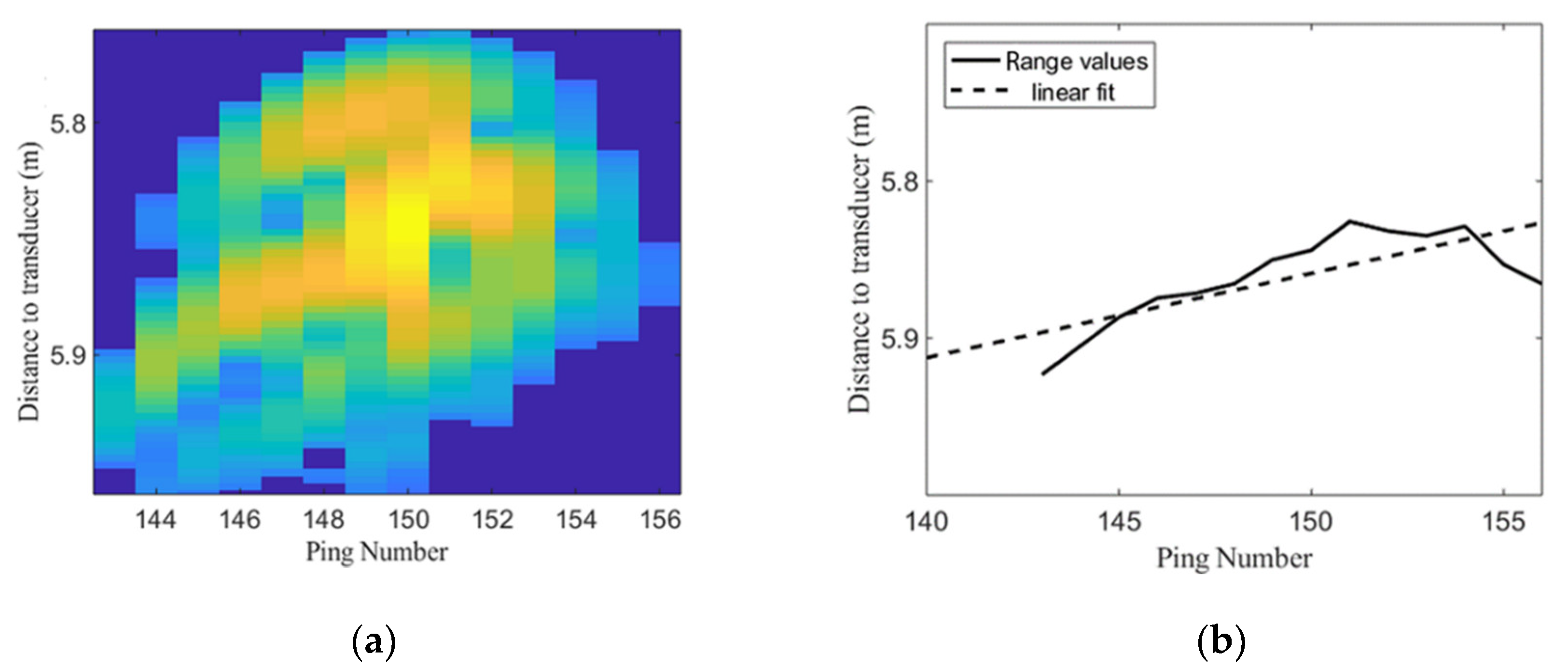
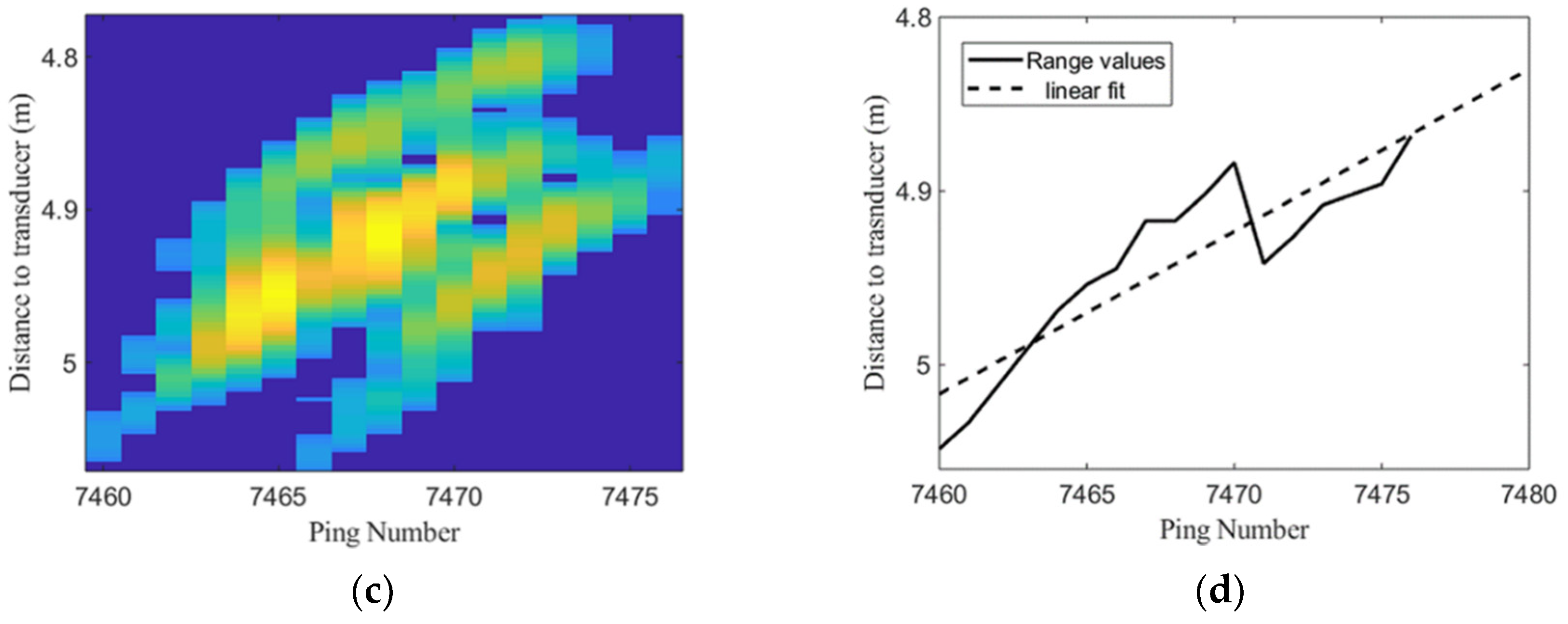
2.2. Acoustic Data Processing for Trace Identification and Characterization
2.3. Optical Data Processing for Fish Sizing in Images
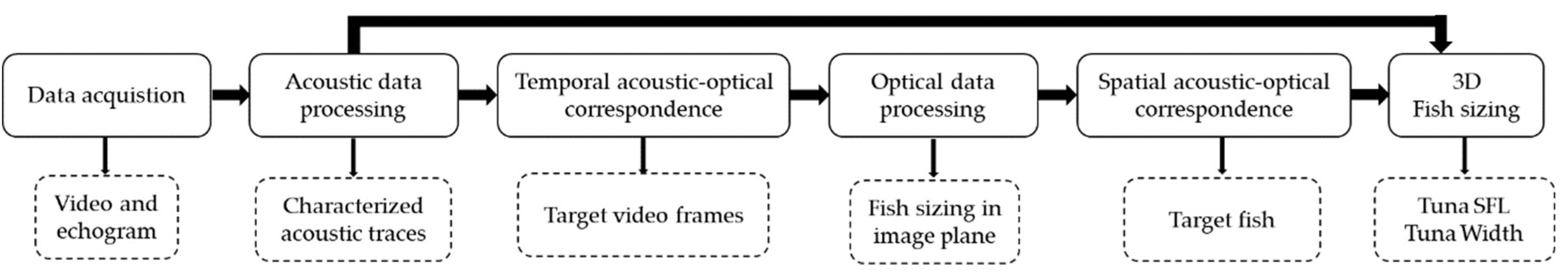
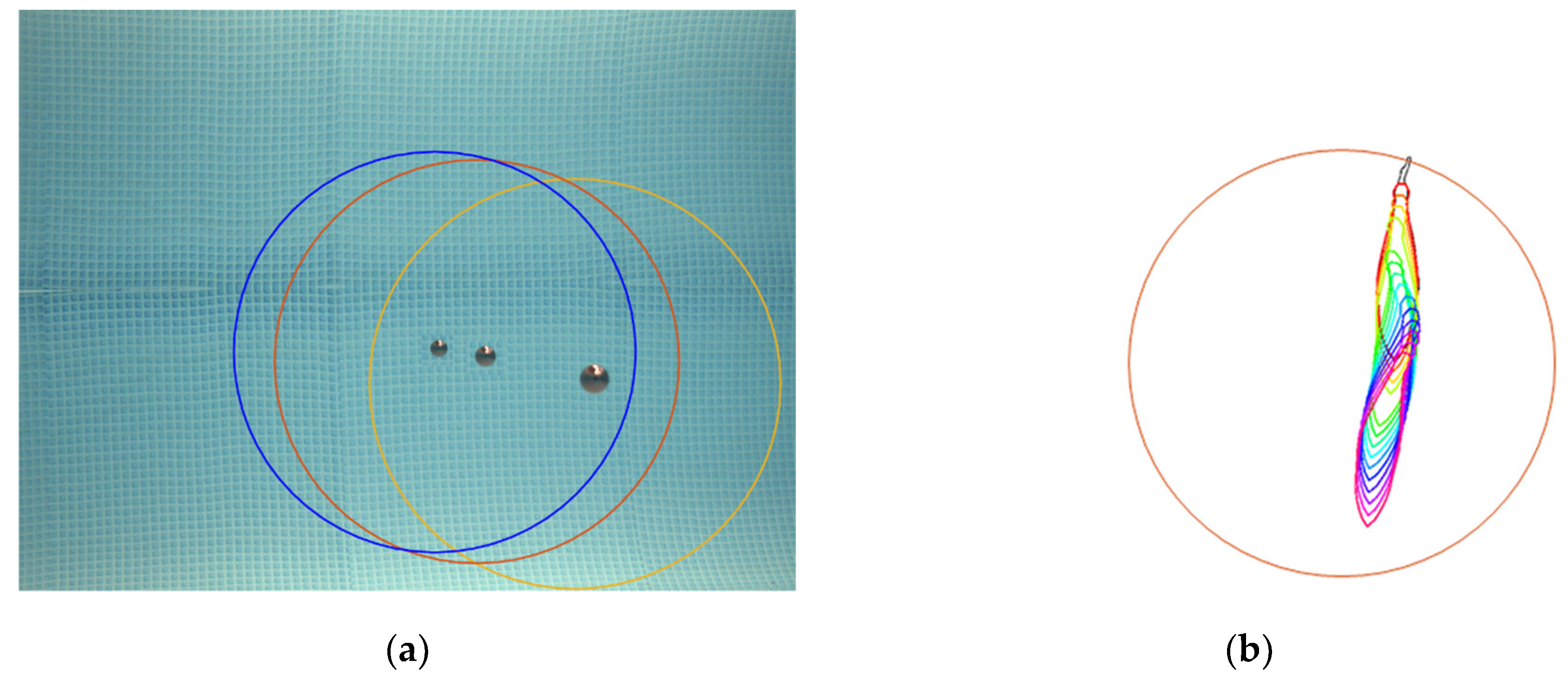
2.4. Combination of Acoustic and Optical Processing for 3D Fish Sizing
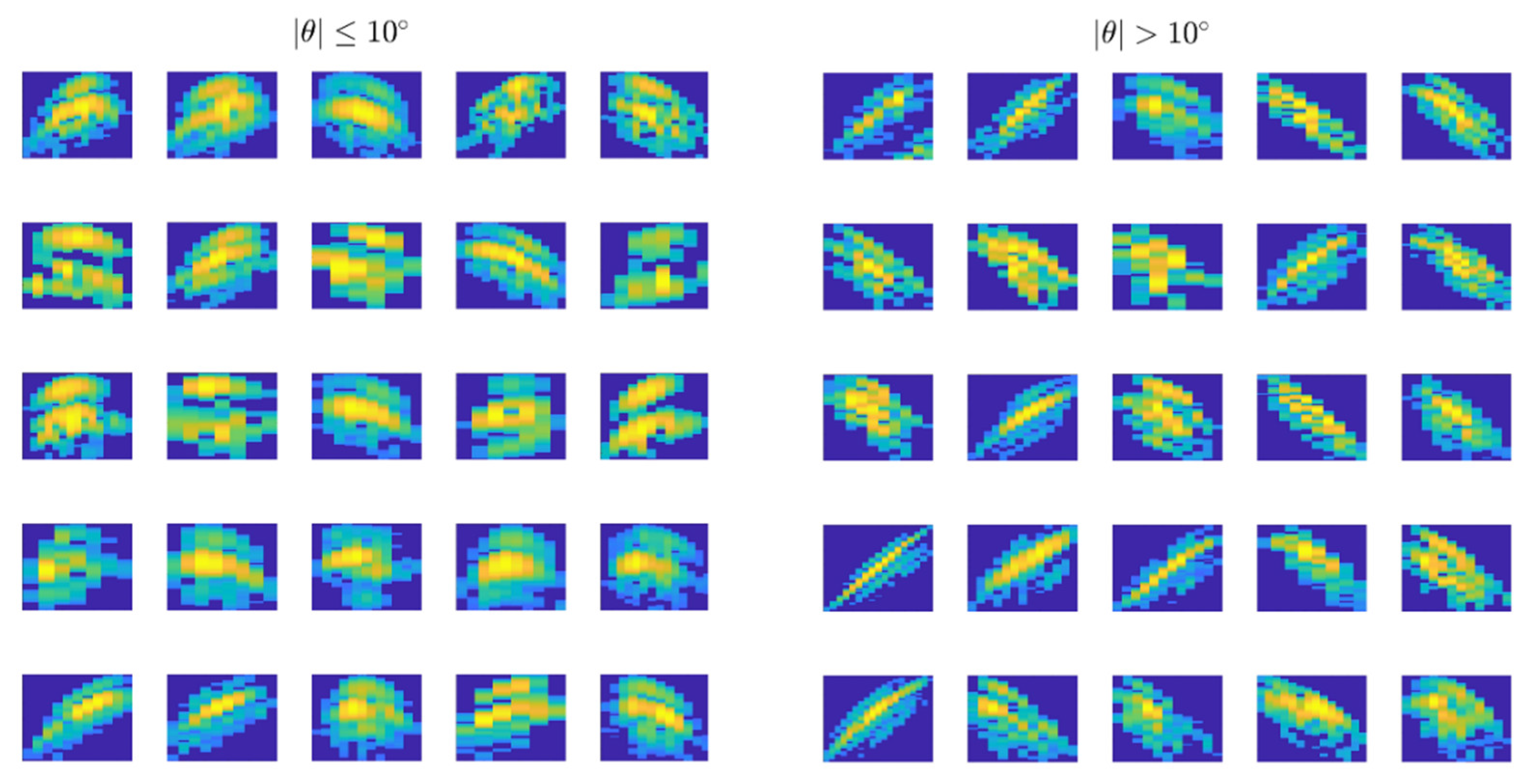
2.5. Discarding Measurements with High Swimming Tilt Angle
3. Results
3.1. Accuracy Analysis
3.2. Computational Cost and Number of Measurements
3.3. Stock Biomass Estimation
4. Conclusions
Author Contributions
Funding
Acknowledgments
Conflicts of Interest
References
- Sawada, K.; Takahashi, H.; Abe, K.; Ichii, T.; Watanabe, K.; Takao, Y. Target-strength, length, and tilt-angle measurements of Pacific saury (Cololabis saira) and Japanese anchovy (Engraulis japonicus) using an acoustic-optical system. ICES J. Mar. Sci. 2009, 66, 1212–1218. [Google Scholar] [CrossRef]
- Kloser, R.J.; Ryan, T.E.; Macaulay, G.J.; Lewis, M.E. In situ measurements of target strength with optical and model verification: A case study for blue grenadier, Macruronus novaezelandiae. ICES J. Mar. Sci. 2011, 68, 1986–1995. [Google Scholar] [CrossRef]
- Zion, B. The use of computer vision technologies in aquaculture—A review. Comput. Electron. Agric. 2012, 88, 125–132. [Google Scholar] [CrossRef]
- Shortis, M.R.; Ravanbakhsh, M.; Shafait, F.; Mian, A. Progress in the Automated Identification, Measurement, and Counting of Fish in Underwater Image Sequences. Mar. Technol. Soc. J. 2016, 50, 4–16. [Google Scholar] [CrossRef]
- Saberioon, M.; Gholizadeh, A.; Cisar, P.; Pautsina, A.; Urban, J. Application of machine vision systems in aquaculture with emphasis on fish: State-of-the-art and key issues. Rev. Aquac. 2017, 9, 369–397. [Google Scholar] [CrossRef]
- Puig-Pons, V.; Muñoz-Benavent, P.; Espinosa, V.; Andreu-García, G.; Valiente-González, J.M.; Estruch, V.D.; Ordóñez, P.; Pérez-Arjona, I.; Atienza, V.; Mèlich, B.; et al. Automatic Bluefin Tuna (Thunnus thynnus) biomass estimation during transfers using acoustic and computer vision techniques. Aquac. Eng. 2019, 85, 22–31. [Google Scholar] [CrossRef]
- Compendium Management Recommendations and Resolutions Adopted by ICCAT for Conservation of Atlantic Tunas and Tuna-Like Species; ICCAT: Madrid, Spain, 2014; ICCAT Recommendation by ICCAT amending the recommendation 13-07 by ICCAT to establish a multi-annual recovery plan for Bluefin Tuna in the eastern Atlantic and Mediterranean; pp. 47–82.
- Shafait, F.; Harvey, E.S.; Shortis, M.R.; Mian, A.; Ravanbakhsh, M.; Seager, J.W.; Culverhouse, P.F.; Cline, D.E.; Edgington, D.R. Towards automating underwater measurement of fish length: A comparison of semi-automatic and manual stereo—Video measurements. ICES J. Mar. Sci. 2017, 74, 1690–1701. [Google Scholar] [CrossRef]
- Lines, J.A.; Tillett, R.D.; Ross, L.G.; Chan, D.; Hockaday, S.; McFarlane, N.J.B. An automatic image-based system for estimating the mass of free-swimming fish. Comput. Electron. Agric. 2001, 31, 151–168. [Google Scholar] [CrossRef]
- Atienza-Vanacloig, V.; Andreu-García, G.; López-García, F.; Valiente-Gonzólez, J.M.; Puig-Pons, V. Vision-based discrimination of tuna individuals in grow-out cages through a fish bending model. Comput. Electron. Agric. 2016, 130, 142–150. [Google Scholar] [CrossRef]
- Phillips, K.; Rodriguez, V.B.; Harvey, E.; Ellis, D.; Seager, J.; Begg, G.; Hender, J. Assessing the Operational Feasibility of Stereo-Video and Evaluating Monitoring Options for the Southern Bluefin Tuna Fishery Ranch Sector; Fisheries Research and Development Corporation Report: Canberra, Australia, 2009. [Google Scholar]
- Shieh, A.C.R.; Petrell, R.J. Measurement of fish size in atlantic salmon (salmo salar l.) cages using stereographic video techniques. Aquac. Eng. 1998, 17, 29–43. [Google Scholar] [CrossRef]
- Difford, G.F.; Boison, S.A.; Khaw, H.L.; Gjerde, B. Validating non-invasive growth measurements on individual Atlantic salmon in sea cages using diode frames. Comput. Electron. Agric. 2020, 173. [Google Scholar] [CrossRef]
- Folkedal, O.; Stien, L.H.; Nilsson, J.; Torgersen, T.; Fosseidengen, J.E.; Oppedal, F. Sea caged Atlantic salmon display size-dependent swimming depth. Aquat. Living Resour. 2012, 25, 143–149. [Google Scholar] [CrossRef]
- Carrera, P.; Churnside, J.H.; Boyra, G.; Marques, V.; Scalabrin, C.; Uriarte, A. Comparison of airborne lidar with echosounders: A case study in the coastal Atlantic waters of southern Europe. ICES J. Mar. Sci. 2006, 63, 1736–1750. [Google Scholar] [CrossRef]
- Mueller, R.P.; Brown, R.S.; Hop, H.; Moulton, L. Video and acoustic camera techniques for studying fish under ice: A review and comparison. Rev. Fish Biol. Fish. 2006, 16, 213–226. [Google Scholar] [CrossRef]
- Mizuno, K.; Liu, X.; Asada, A.; Ashizawa, J.; Fujimoto, Y.; Shimada, T. Application of a high-resolution acoustic video camera to fish classification: An experimental study. In Proceedings of the 2015 IEEE Underwater Technology, Chennai, India, 23–25 February 2015. [Google Scholar]
- Espinosa, V.; Soliveres, E.; Cebrecos, A.; Puig, V.; Sainz-Pardo, S.; de la Gándara, F. Growing Monitoring in Sea Cages: Ts Measurements Issues. In Proceedings of the 34th Scandinavian Symposium on Physical Acoustics, Geilo, Norway, 30 January–2 February 2011. [Google Scholar]
- Harvey, E.; Cappo, M.; Shortis, M.; Robson, S.; Buchanan, J.; Speare, P. The accuracy and precision of underwater measurements of length and maximum body depth of southern bluefin tuna (Thunnus maccoyii) with a stereo-video camera system. Fish. Res. 2003, 63, 315–326. [Google Scholar] [CrossRef]
- Muñoz-Benavent, P.; Andreu-García, G.; Valiente-González, J.M.; Atienza-Vanacloig, V.; Puig-Pons, V.; Espinosa, V. Automatic Bluefin Tuna sizing using a stereoscopic vision system. ICES J. Mar. Sci. 2018, 75, 390–401. [Google Scholar] [CrossRef]
- Muñoz-Benavent, P.; Andreu-García, G.; Valiente-González, J.M.; Atienza-Vanacloig, V.; Puig-Pons, V.; Espinosa, V. Enhanced fish bending model for automatic tuna sizing using computer vision. Comput. Electron. Agric. 2018, 150, 52–61. [Google Scholar] [CrossRef]
- Fan, J.; Huang, Y.; Shan, J.; Zhang, S.; Zhu, F. Extrinsic calibration between a camera and a 2D laser rangefinder using a photogrammetric control field. Sensors 2019, 19, 2030. [Google Scholar] [CrossRef]
- Wen, C.; Qin, L.; Zhu, Q.; Wang, C.; Li, J. Three-dimensional indoor mobile mapping with fusion of two-dimensional laser scanner and RGB-D camera data. IEEE Geosci. Remote Sens. Lett. 2014, 11, 843–847. [Google Scholar] [CrossRef]
- Sim, S.; Sock, J.; Kwak, K. Indirect Correspondence-Based Robust Extrinsic Calibration of LiDAR and Camera. Sensors 2016, 16, 933. [Google Scholar] [CrossRef]
- Enzenhofer, H.J.; Olsen, N.; Mulligan, T.J. Fixed-location riverine hydroacoustics as a method of enumerating migrating adult Pacific salmon: Comparison of split-beam acoustics vs. visual counting. Aquat. Living Resour. 1998, 11, 61–74. [Google Scholar] [CrossRef]
- Underwood, M.; Sherlock, M.; Marouchos, A.; Cordell, J.; Kloser, R.; Oceans, T.R.; Flagship, A. A combined acoustic and optical instrument for industry managed fisheries studies. In Proceedings of the MTS/IEEE OCEANS 2015—Genova: Discovering Sustainable Ocean Energy for a New World, Genoa, Italy, 18–21 May 2015. [Google Scholar]
- Lu, H.J.; Kang, M.; Huang, H.H.; Lai, C.C.; Wu, L.J. Ex situ and in situ measurements of juvenile yellowfin tuna Thunnus albacares target strength. Fish. Sci. 2011, 77, 903–913. [Google Scholar] [CrossRef]
- Rooper, C.N.; Hoff, G.R.; De Robertis, A. Assessing habitat utilization and rockfish ( Sebastes spp.) biomass on an isolated rocky ridge using acoustics and stereo image analysis. Can. J. Fish. Aquat. Sci. 2010, 67, 1658–1670. [Google Scholar] [CrossRef]
- Sawada, K.; Takahashi, H.; Takao, Y.; Watanabe, K.; Horne, J.K.; McClatchie, S.; Abe, K. Development of an acoustic-optical system to estimate target-strengths and tilt angles from fish aggregations. In Proceedings of the Ocean’04—MTS/IEEE Techno-Ocean’04: Bridges across the Oceans, Kobe, Japan, 9–12 November 2004; pp. 395–400. [Google Scholar]
- Ryan, T.E.; Kloser, R.J.; Macaulay, G.J. Measurement and visual verification of fish target strength using an acoustic-optical system attached to a trawlnet. ICES J. Mar. Sci. 2009, 66, 1238–1244. [Google Scholar] [CrossRef]
- Simrad ER60 Scientific Echo Sounder. Reference Manual; Kongsberg Maritime AS: Horten, Norway, 2008.
- Eidson, J.; Lee, K. IEEE 1588 standard for a precision clock synchronization protocol for networked measurement and control systems. In Proceedings of the Sensors for Industry Conference, Houston, TX, USA, 19–21 November 2002; pp. 98–105. [Google Scholar]
- Heikkila, J.; Silven, O. A Four-step Camera Calibration Procedure with Implicit Image Correction. In Proceedings of the 1997 Conference on Computer Vision and Pattern Recognition (CVPR’97), San Juan, PR, USA, 17–19 June 1997; IEEE Computer Society: Washington, DC, USA, 1997; p. 1106. [Google Scholar]
- Zhang, Z. A Flexible New Technique for Camera Calibration. IEEE Trans. Pattern Anal. Mach. Intell. 2000, 22, 1330–1334. [Google Scholar] [CrossRef]
- Otsu, N. A Threshold Selection Method from Gray-Level Histograms. IEEE Trans. Syst. Man. Cybern. 1979, 9, 62–66. [Google Scholar] [CrossRef]
- Petrou, M.; Petrou, C. Image Segmentation and Edge Detection. In Image Processing: The Fundamentals; John Wiley & Sons, Ltd.: Chichester, UK, 2011; pp. 527–668. [Google Scholar]
- Voulodimos, A.; Doulamis, N.; Doulamis, A.; Protopapadakis, E. Deep Learning for Computer Vision: A Brief Review. Comput. Intell. Neurosci. 2018, 2018. [Google Scholar] [CrossRef]
- Guo, Y.; Liu, Y.; Oerlemans, A.; Lao, S.; Wu, S.; Lew, M.S. Deep learning for visual understanding: A review. Neurocomputing 2016, 187, 27–48. [Google Scholar] [CrossRef]
- Kamilaris, A.; Prenafeta-Boldú, F.X. Deep learning in agriculture: A survey. Comput. Electron. Agric. 2018, 147, 70–90. [Google Scholar] [CrossRef]
- Chen, Y.; Lin, Z.; Zhao, X.; Wang, G.; Gu, Y. Deep learning-based classification of hyperspectral data. IEEE J. Sel. Top. Appl. Earth Obs. Remote Sens. 2014, 7, 2094–2107. [Google Scholar] [CrossRef]
- West, J.; Ventura, D.; Warnick, S. Spring research presentation: A theoretical foundation for inductive transfer. Brigham Young Univ. Coll. Phys. Math. Sci. 2007, 1, 10. [Google Scholar]
- Pan, S.J.; Yang, Q. A survey on transfer learning. IEEE Trans. Knowl. Data Eng. 2010, 22, 1345–1359. [Google Scholar] [CrossRef]
- Krizhevsky, A.; Sutskever, I.; Hinton, G.E. ImageNet classification with deep convolutional neural networks. Commun. ACM 2017, 60, 84–90. [Google Scholar] [CrossRef]
- Aguado-Gimenez, F.; Garcia-Garcia, B. Growth, food intake and feed conversion rates in captive Atlantic bluefin tuna (Thunnus thynnus Linnaeus, 1758) under fattening conditions. Aquac. Res. 2005, 36, 610–614. [Google Scholar] [CrossRef]
- Martinez-de Dios, J.R.; Serna, C.; Ollero, A. Computer vision and robotics techniques in fish farms. Robotica 2003, 21, 233–243. [Google Scholar] [CrossRef]
- Puig-Pons, V.; Estruch, V.D.; Espinosa, V.; De La Gándara, F.; Melich, B.; Cort, J.L. Relationship between weight and linear dimensions of bluefin tuna (thunnus thynnus) following fattening on western mediterranean farms. PLoS ONE 2018, 13, e0200406. [Google Scholar] [CrossRef]
- Costa, C.; Scardi, M.; Vitalini, V.; Cataudella, S. A dual camera system for counting and sizing Northern Bluefin Tuna (Thunnus thynnus; Linnaeus, 1758) stock, during transfer to aquaculture cages, with a semi automatic Artificial Neural Network tool. Aquaculture 2009, 291, 161–167. [Google Scholar] [CrossRef]
- Serikawa, S.; Lu, H. Underwater image dehazing using joint trilateral filter. Comput. Electr. Eng. 2014, 40, 41–50. [Google Scholar] [CrossRef]


| Tilted Samples |θ| > 10° | Non-Tilted Samples |θ| ≤ 10° | |||
|---|---|---|---|---|
| True Positives | False Positives | True Positives | ||
| STI | 522/828 (63%) | 306/828 (37%) | 3486/5203 (67%) | |
| 588/828 (71%) | 240/828 (29%) | 2914/5203 (56%) | ||
| CNN | NT = 200 | 540/628 (86%) | 88/628 (14%) | 4253/5003 (85%) |
| NT = 50 | 650/778 (83.5%) | 128/778 (16.5%) | 4225/5153 (82%) | |
| MAY | SEPTEMBER | ||||
|---|---|---|---|---|---|
| |θ| > 10° | |θ| ≤ 10° | |θ| > 10° | |θ| ≤ 10° | ||
| STI | 62.2% | 67.2% | 63.8% | 66.7% | |
| 70.2% | 56.7% | 71.7% | 55.4% | ||
| CNN | NT = 200 | 87.7% | 86.9% | 84.5% | 82.3% |
| NT = 50 | 82.4% | 83.5% | 84.6% | 79.4% | |
| MAY | SEPTEMBER | TOTAL | ||||
|---|---|---|---|---|---|---|
| AO SENSOR | STEREO SYSTEM | AO SENSOR | STEREO SYSTEM | AO SENSOR | STEREO SYSTEM | |
| Recording time | 33 h | 50 h | 83 h | |||
| NM | 2894 | 11,038 | 2136 | 10,603 | 5030 | 21,641 |
| NMHR | 88 samples/h | 335 samples/h | 42.7 samples/h | 212 samples/h | 60.6 samples/h | 261 samples/h |
| Computing time | 30 h | 924 h (38.5 days) | 45 h | 1400 h (58.3 days) | 75 h | 2324 (96.8 days) |
| NMHC | 96.5 samples/h | 11.9 samples/h | 47.5 samples/h | 7.6 samples/h | 67.1 samples/h | 9.3 samples/h |
| MAY | SEPTEMBER | ||||
|---|---|---|---|---|---|
| STEREO SYSTEM | AO SENSOR | STEREO SYSTEM | AO SENSOR | ||
| NM | 11,038 | 2894 | 10,603 | 2136 | |
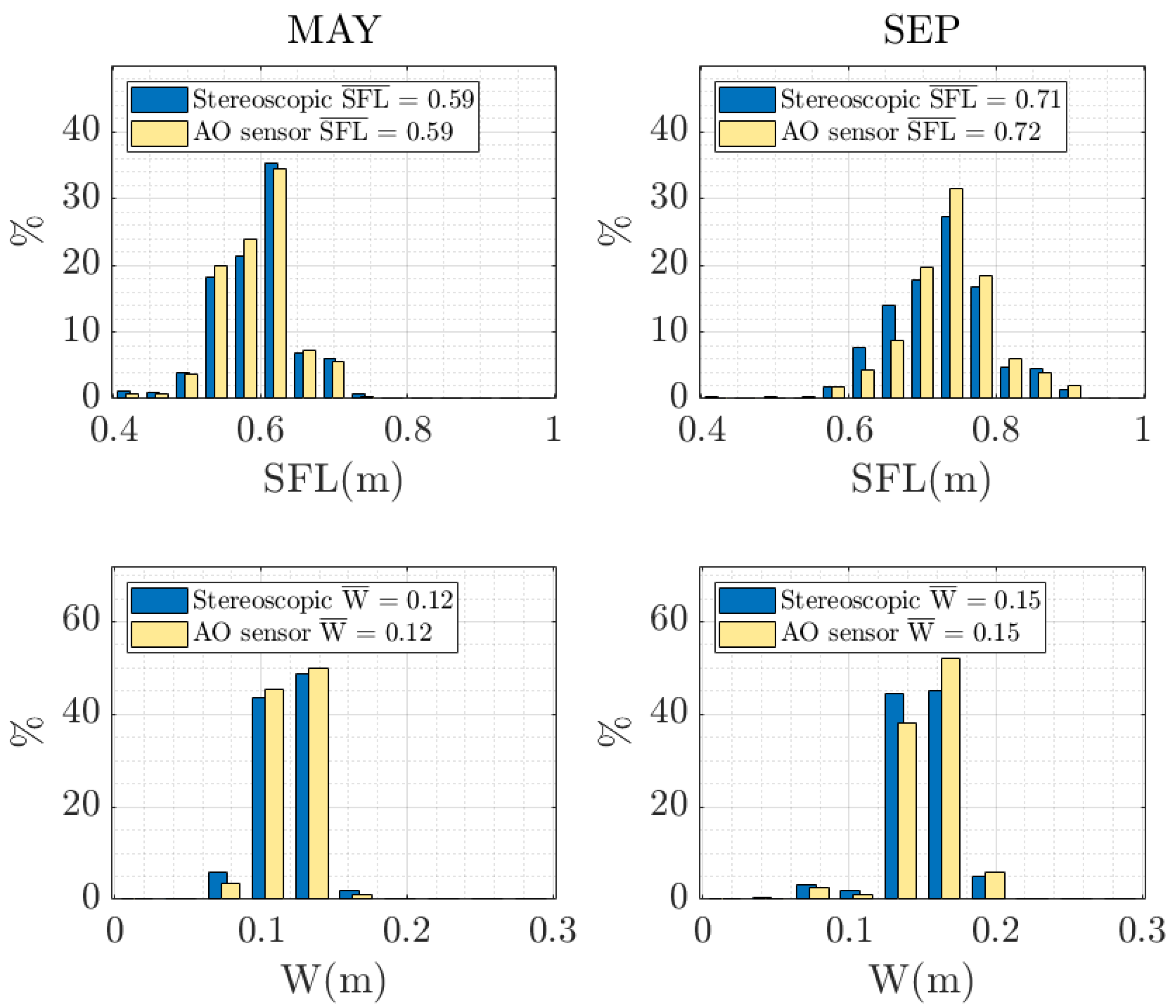
| SFL | µ | 0.59 | 0.59 | 0.71 | 0.72 |
| σ | 0.0761 | 0.0676 | 0.0907 | 0.0930 | |
| σ2 | 0.0058 | 0.0046 | 0.0082 | 0.0086 | |
| W | µ | 0.12 | 0.12 | 0.15 | 0.15 |
| σ | 0.0170 | 0.0154 | 0.0228 | 0.0225 | |
| σ2 | 2.88 × 10⁻⁴ | 2.4 × 10⁻⁴ | 5.20 × 10⁻⁴ | 5.06 × 10⁻⁴ | |
© 2020 by the authors. Licensee MDPI, Basel, Switzerland. This article is an open access article distributed under the terms and conditions of the Creative Commons Attribution (CC BY) license (http://creativecommons.org/licenses/by/4.0/).
Share and Cite
Muñoz-Benavent, P.; Puig-Pons, V.; Andreu-García, G.; Espinosa, V.; Atienza-Vanacloig, V.; Pérez-Arjona, I. Automatic Bluefin Tuna Sizing with a Combined Acoustic and Optical Sensor. Sensors 2020, 20, 5294. https://doi.org/10.3390/s20185294
Muñoz-Benavent P, Puig-Pons V, Andreu-García G, Espinosa V, Atienza-Vanacloig V, Pérez-Arjona I. Automatic Bluefin Tuna Sizing with a Combined Acoustic and Optical Sensor. Sensors. 2020; 20(18):5294. https://doi.org/10.3390/s20185294
Chicago/Turabian StyleMuñoz-Benavent, Pau, Vicente Puig-Pons, Gabriela Andreu-García, Víctor Espinosa, Vicente Atienza-Vanacloig, and Isabel Pérez-Arjona. 2020. "Automatic Bluefin Tuna Sizing with a Combined Acoustic and Optical Sensor" Sensors 20, no. 18: 5294. https://doi.org/10.3390/s20185294
APA StyleMuñoz-Benavent, P., Puig-Pons, V., Andreu-García, G., Espinosa, V., Atienza-Vanacloig, V., & Pérez-Arjona, I. (2020). Automatic Bluefin Tuna Sizing with a Combined Acoustic and Optical Sensor. Sensors, 20(18), 5294. https://doi.org/10.3390/s20185294