1. Introduction
The incident angle of the electromagnetic (EM) wave relative to the receiver is called direction of arrival (DOA). In radar, communication, radio astronomy, telemetry, track and command, and other fields [
1,
2,
3], users always need to estimate the DOA of EM waves. For example, the DOA information wave can be used in the beam control system of the receiver antenna, so that the main beam of the receiver antenna can track the incident signal all the time. Different DOA estimation methods are adopted in various application fields. Each method has its own advantages and keeps developing continuously.
Nowadays, the most traditional DOA estimation equipment is the interferometer, which estimates the DOA according to the phase difference between EM waves received by adjacent antenna elements. The phase difference is caused by the difference in distance between the radiation source and different antenna elements, and it has a certain geometric relationship with the incident angle. However, there are some shortcomings in DOA estimation of the interferometer. Firstly, the estimation accuracy is not high because the algorithm is vulnerable to noise. Obtaining the phase difference is a key step for interferometer. Common methods include zero-crossing detection, Fast Fourier Transform (FFT) [
4], and Hilbert orthogonal transformation [
5] and so on. The zero-crossing detection uses the approximation of the function near the zero point, i.e., sin
x =
x, to accurately determine the zero-crossing position of the sample sequence. These positions can help to calculate the path difference between the signals received by different antenna elements. Unfortunately, noise results in serious uncertainty when estimating the zero point. In addition to noise, the estimation accuracy is also related to the sample frequency of the signal, which requires high performance of the hardware. FFT is another way to estimate the phase difference between signals. The phase difference between the two signals can be easily obtained by FFT and cross-correlation operation on the sample sequence. Compared with zero-crossing detection, the FFT-based algorithm performs much better in anti-noise and anti-harmonic interference, so it could achieve higher accuracy in the phase difference estimation. The second shortcoming for the interferometer is that the estimation accuracy is closely related to the array spacing. The shortest interval in an interferometer array is usually less than half a wavelength; hence, the phase measured in this case is unique [
6,
7]. However, in broadband direction-finding systems over a range such as 0.1–3 GHz or 2–8 GHz, the physical dimensions of the antenna element are dictated by the lowest operating frequency, whereas the shortest interelement spacing is decided by the highest frequency. This poses the problem of not being able to employ a short spacing of less than half-wavelength [
8,
9]. However, if the baseline length exceeds the half-wavelength of the pulse signal, the periodic ambiguity will be introduced into the phase measurement and its ambiguity is 2π. The combination of long baseline and short baseline is an effective method to solve the phase ambiguity. Even so, the combination of multiple baselines greatly increases the complexity of the system and requires more accurate calibration of the system. Thirdly, the interferometer can only aim at a single signal in the main lobe, and cannot be used when multiple EM waves arrive at the antenna at the same time. In this case, it means insufficient resolution.
In order to promote the resolution and realize the DOA estimation of multiple incident signals, various methods based on antenna arrays have become the research hotspot in the last decades. So far, several classes of DOA estimation techniques for incoherently distributed sources have been developed, such as the subspace method and the parameter method. Multiple Signal Classification (MUSIC) and Estimating Signal Parameter via Rotational Invariance Techniques (ESPRIT) are the most important subspace methods [
10,
11,
12]. Furthermore, the maximum likelihood (ML) algorithm [
13,
14] and Covariance Matching Estimator (COMET) algorithm [
15,
16] are typical parameter estimation approaches, which can obtain better estimation performance than subspace methods. However, their computing load is also heavier. Meanwhile, DOA estimation methods based on antenna arrays are facing two great challenges. First, the complexity of the algorithm is too high to implement from an engineering perspective. In these technologies, most methods are proposed for uniform linear arrays; therefore, the spectral peak search happens only on a two-dimensional plane, which makes it impossible to estimate the elevation angle and azimuth angle simultaneously. Later, researchers further developed these algorithms to make them suitable for planar arrays. In this way, the range of the spectral peak search is extended to three-dimensional space, which means that the DOA of the signal source can completely include both the elevation angle and azimuth angle. However, due to multi-dimensional space spectrum search, a large amount of computational burden has always been a problem that researchers need to solve [
17]. In addition to the huge computation of the spectral peak search, this kind of DOA algorithm involves various complex operations such as matrix eigenvalue decomposition, which resulting in difficulties in the engineering implementation of programmable devices, such as FPGA. Another challenge is that these antenna arrays generally have a large number of elements and each element needs a corresponding radio frequency front-end channel, which makes the hardware cost very high.
Different from the popular algorithms mentioned above, we use a tripole vector antenna to make full use of the electric field of the EM wave and develop a fast DOA estimation algorithm for a single signal. The tripole vector antenna is also known as a polarization sensitive antenna, which is different from the traditional single polarization antenna because it can accurately sense the polarization characteristics of EM waves [
18]. The tripole vector antenna is proposed by R.T Compton [
19,
20], and it is composed of three orthogonal dipole antennas. Document [
21] proposed a DOA estimation method based on polarization-spatial steering vector. It uses a tripole antenna but needs to know the elliptical susceptibility of the polarized signal. In recent years, polarization-sensitive arrays have become the focus of academic research, where each element is one tripole vector antenna. Researchers try to achieve higher performance through polarization-sensitive arrays in the fields of spatial spectrum estimation and adaptive anti-jamming array. In fact, it is a signal processing method combining spatial and polarimetry resources, which improves the array freedom degree of the receiver. For example, the tripole antenna has been proposed as one possible choice of antenna construction to be used in the low-frequency array (LOFAR) project [
22]. The primary field of application for the project is radio-based astrophysics.
Due to the structural characteristics of the tripole vector antenna, we only need to use one tripole vector antenna to complete the DOA estimation of the EM wave if there is only one signal in space. We map the sample data of the tripole vector antenna to the space rectangular coordinate system and calculate the DOA by vector product according to the geometric relationship. The new method has some obvious advantages over the other methods. First of all, the proposed DOA algorithm does not need to solve equations such as the interferometer or search the spectral peak such as array signal processing methods [
23]; as a result, the signal processing process is much simpler. Secondly, the main lobe of the tripole vector antenna is wide enough so that any signal impinging from the main lobe area could be captured and no servo system is needed. Obviously, this reduces the cost of hardware greatly. Thirdly, the DOA estimation method based on the tripole vector antenna is suitable for any nonlinearly polarized EM wave without any polarization-matching problem between antennas and EM waves, because it captures all the polarization information of EM waves. This is also the advantage that other DOA estimation methods do not have. Similar to the interferometer, the new method also has the disadvantage of insufficient resolution, but it can be solved by combining with other subspace estimation algorithms.
The rest of this paper is as follows.
Section 2 is a brief introduction of the received signal model.
Section 3 is the overall description of the method. The method complexity and error analysis are discussed in
Section 4. The experimental results of different methods are presented in
Section 5.
Section 6 concludes the paper.
2. Signal Model
The tripole vector antenna is composed of three identical and mutually perpendicular linearly polarized dipole antennas centered at the same position [
19,
20,
21], as shown in
Figure 1. Each linearly polarized dipole antenna can only receive the electric field component in its polarization direction and has an output feed point. The polarization direction of the dipoles in a tripole are respectively parallel to the three coordinate axes of the space rectangular coordinate system, which ensures that no matter which direction the EM wave is incident from, and no matter what polarization the EM wave is, all the energy of the EM wave can be received by the tripole vector antenna. So, there will be no polarization-matching problem. In addition, since all three feed points are concentrated at the same location, phase shifts between units will not occur in a tripole vector antenna.
In the coordinate system shown in
Figure 1, we suppose that the DOA of an elliptically polarized EM wave signal is incident from a certain direction. Once the signal reaches the antenna, its electric field will be simultaneously received by the three orthogonal dipoles of the antenna. We name the three poles of the antenna as
x,
y,
z, hence the signal received by the antenna can be expressed as
where
Exm,
Eym, and
Ezm and
ϕx,
ϕy, and
ϕz are the amplitudes and initial phases of the electric field components in the
x,
y, and
z directions.
nx(
n),
ny(
n), and
nz(
n) are independent white Gaussian noise in the
x,
y, and
z directions.
n is the sample number,
Ts is the sample period, and
ω is the angular frequency of the EM wave.
4. Performance Analysis
4.1. Probability Distribution of Estimated Angles
Since there is noise in the snapshot, the estimated angles and are considered as random variables. In order to find out the Probability Density Function (PDF), the PDFs of mx, my, and mz need to be calculated first.
Considering noise components in received signals, we plug Equations (1)–(3) into Equations (8)–(10) respectively, and obtain
mx,
my, and
mz with noise. Since the three variables have the same structure, only the PDF of
mx is analyzed. For
mx, which can be expanded as
where
Obviously, mx0 is ideal value without noise, but Px and Qx have noise. Apparently, noise snapshot nx, ny, and nz are Gaussian random variables with a mean 0 and variance , , and respectively.
Since
Qx is the sum of multiple independent Gaussian random variables,
Qx is also a random variable of Gaussian distribution. According to Equation (22), it is not difficult to find out the mean and variance are respectively:
Therefore, the PDF of
Qx is:
In order to obtain the PDF of Px, two related theorems are given in advance.
Theorem 1. If two independent random variables x and y obey the Gaussian distribution with mean 0 and variance,the PDF of the variable z = xy is:
where the function K0 is the modified Bessel function of the second kind of order 0. Theorem 2 [22].If the PDFs of two independent random variables x and y are fx(x) and fy(y) respectively, the PDF of the variable z = x + y is:
Looking back to Equation (21), function
Px is the difference of two independent components, and each independent component is the product of two independent Gaussian variables. Hence, using Theorems 1 and 2, we can get the PDF of the variable
Px:
According to Equation (19), and using Theorem 2 again, we can get the PDF of variable
mx; similarly, we can get PDFs of
my,
mz.
According to Equation (24), similarly, we can define
,
as follows
In order to simplify Equations (29)–(31), we replace exp(−|t|) with a function, which fits well with the original function. This alternative function is
where
a1 = 0.4652,
b1 = 0.5524,
a2 = 0.4396,
b2 = 1.911, and max |exp(−|t|) −
h(
t)| is less than 0.03, which means these two functions fit well.
In this way, Equations (29)–(31) can be replaced as:
In order to get PDFs of and , we quote two more related theorems.
Theorem 3 [22].If, andis the inverse function of u on z, u has continuous partial derivative to x, y, z, the joint PDF of x, y, z is, hence the PDF of u is Theorem 4 [22].If, andis the inverse function of u on y, u has continuous partial derivative to x, y, the joint PDF of x, y is, hence the PDF of u is If we define the joint PDF of random variables (
mx,
my,
mz) is
f1(
mx,
my,
mz), then
Replacing
mx,
my, and
mz with
x,
y, and
z, according to Equation (12) and Theorem 3, the PDF of the estimated elevation angle
can be obtained as
where
In the same way, if the joint PDF of random variables (
mx,
my) is
according to Equation (15) and Theorem 4, the PDF of the estimated azimuth
can be obtained as
where
Hence
after simplification,
where
and
Clearly,
is a cumulative distribution function of the standard normal distribution with an integral. For the sake of simplicity, we use function I(x) to replace
if max|
− I(
x)| is less than 0.01,
4.2. Statistical Characteristics of Angle Estimatior
The statistical characteristics of angle estimators are the main indicators to measure the estimation performance. In order to analyze the statistical characteristics of angle estimates, we first study the distribution characteristics of the vector
, which is obtained by Equation (16). According to
Section 4.1, the estimated
is symmetrically distributed in space about the accurate value
m0; as a result, the mean value of
should be equal to the accurate value
m0, namely
Meanwhile, let
,
and
as the variance of
mx,
my, and
mz and
,
and
as the variance of
,
and
according to the relationship among variables above, we can obtain
Obviously, when the number of snapshots K tends to infinity, , and are all close to 0.
According to above conclusion, using Chebyshev’s theorem, the following inequalities are established:
where
ε1,
ε2, and
ε3 are arbitrary positive numbers.
Clearly, the probability for
,
and
deviate from
mx0,
my0, and
mz0 tends to 0 respectively if the number of snapshots
K is very large. Combining Equations (16) and (17), we can get
Therefore, we can conclude that our algorithm is an asymptotic unbiased estimation, and the estimated value will become closer to the true value as the number of snapshots increases.
4.3. Analysis of Algorithm Complexity
MUSIC is a DOA estimation method based on subspace, which uses eigenvalue decomposition to the covariance matrix and searches peaks by spatial spectrum. Its advantage is that D different signals can be estimated at the same time. However, the disadvantage is that the N-element array must be used and results in heavy computation load, where N > D.
The computation load of the interferometer algorithm is relatively small, but the amount of operation increases significantly with the number of array elements. In addition, if the correction for amplitude and phase errors is considered, the amount of operation would further increase.
Compared with above these two algorithms, the proposed algorithm based on a tripole vector antenna has a significant advantage in computation. When K snapshots are used for estimation, the new algorithm here only needs to complete multiplication in 6K − 1 times, addition in 6K − 1 times, division in 2 times, square root in 2 times, and anti-cosine function in 2 times.
In details, the square root operation is calculated by Newton iterative method, and the iterative formula is
where
b is a radicand. Since
A means iteration times and
xA is the square root of
b, there are
A times of addition,
A times of multiplication, and
A times of division in one square root operation. On the other hand, we calculate the inverse cosine function by Taylor’s expansion
So, the amount of an anti-cosine function computation consists of (M + 1) (M + 2) times of multiplication, times of addition.
In conclusion, the computation load of the proposed algorithm includes
M2 + 3
M + 1 + 2
A + 6
K times of multiplication,
n + 2
A + 6
K times of addition, 2 + 2
A times of division. The computation load of each algorithm can be seen in
Table 1.
Where Q is spectral peak search times of azimuth and I is that of elevation.
It can be seen from
Table 1 that compared with existing methods, our algorithm of angle estimation based on a single tripole vector antenna has obvious advantages in computational complexity.
5. Simulations
In this section, we present some numerical results to assess the performance of our algorithm. For a comparison, we investigate the performance of MUSIC [
11], Interferometer [
9], and our proposed algorithm.
In the following simulations, we consider an L-shaped array consisting of three parallel dipoles used for the interferometer, and three triple vector antennas used for both MUSIC and the proposed algorithm. The spectral peak search interval of the MUSIC algorithm is 0.1 degree. In addition, we assume that the DOA of the incident EM wave is , and the frequency of the EM wave is 1 GHz.
For a statistical comparison, we define the root mean square error (RMSE) as
where
and
are the actual values of azimuth and elevation angle, respectively. In addition,
and
are the estimated values of azimuth and elevation angle in the
j-th Monte Carlo trial where
j = 1, 2, ...,
J.
We also consider the statistical characteristics of the estimation error for the proposed algorithm. The estimation error is defined as the difference between the estimated value and true value, that is
Their mean and variance are
In addition, the signal-to-noise ratio is defined as
where
Ps and
Pn represent the effective power of signal and noise, respectively.
5.1. Simulation 1: Statistical Characteristics of Angle Error
In the first simulation, we mainly introduce the statistical characteristics of the estimation error of the proposed algorithm according to Equations (71) and (72). Supposing
J = 200 and SNR = 10 dB, the results are shown in
Figure 4.
In
Figure 4, the mean of the estimation error is almost always 0 even in the case of small number of snapshots, which illustrates that the estimation method can be considered unbiased and the error mean is not sensitive to the number of snapshots. However, the variance of estimation error is relatively large when the number of snapshots is small. Increasing the number of snapshots can reduce the variance. Furthermore, the variance of azimuth is always larger than that of elevation angle.
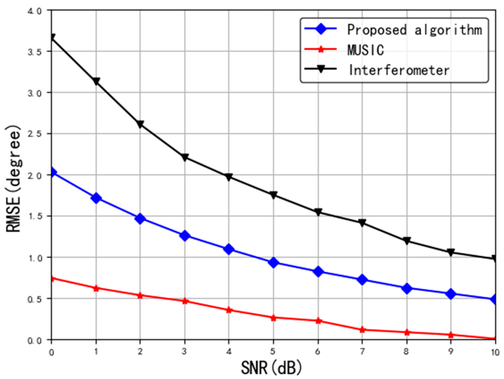
5.2. Simulation 2: Comparison of RMSE Performance Versus Different SNR
The second simulation illustrates the comparison of the performance among three kinds of DOA estimation algorithms, which are phase interferometer, MUSIC, and the proposed tripole vector antenna method. In the simulation,
K = 1000,
J = 200, and SNR varies from 0 to 10 dB. The results are shown in
Figure 5.
It depicts in
Figure 5 that the MUSIC algorithm has the best performance followed by the proposed algorithm here. In addition, due to the polarization mismatch between the EM wave and the antenna for interferometer, the input SNR loss is 3 dB and leads to an estimation error almost twice that of the proposed method.
5.3. Simulation 3: Comparison of RMSE Performance Versus Different Snapshots
The third simulation compares the performance of the three algorithms under different snapshots. In this simulation, SNR = 10 dB,
J = 200, and
K varies from 100 to 1000. The results are shown in
Figure 6.
As illustrated in
Figure 6, when the number of snapshots is the same, the performance of MUSIC is the best, followed by the proposed algorithm and the interferometer. This result is very similar to the simulation result in
Section 5.2, which shows that increasing number of snapshots is equal to improving the SNR for the proposed algorithm.
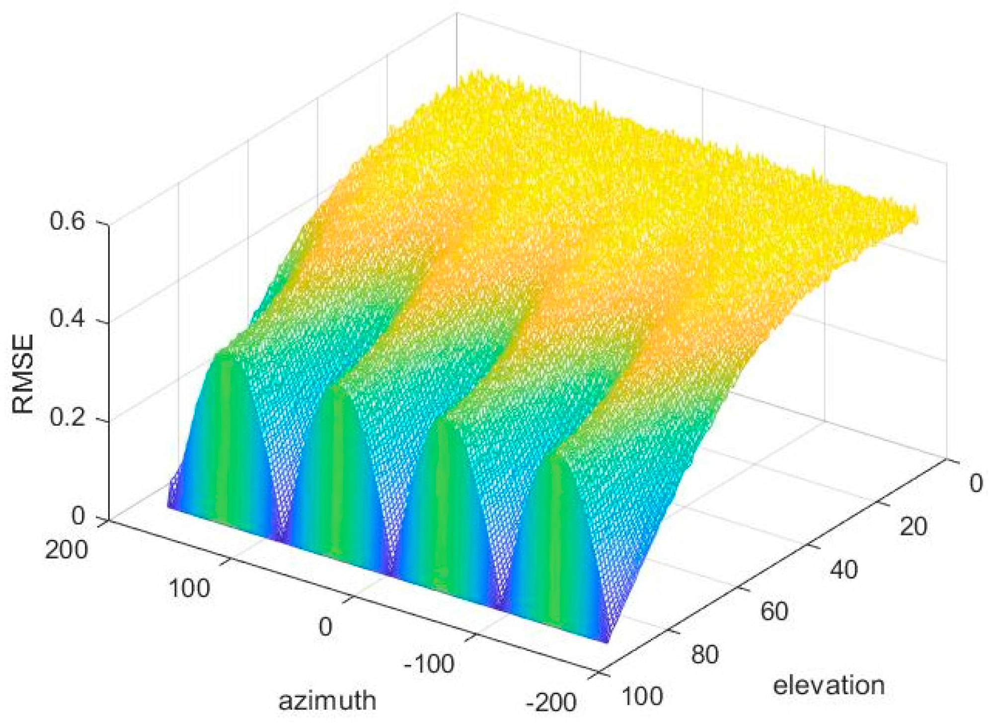
5.4. Simulation 4: RMSE for Different DOAs in Degrees
In order to fully demonstrate the estimated performance of the proposed algorithm at various angles, we simulated all angles under the condition of 10 dB and 1000 snapshots, and the results are as follows.
According to
Figure 7, estimate errors are different in various incident angles. In the situation of invariant azimuth, as a decline of elevation, RMSE decreases; when the elevation stays invariant, the RMSE varies periodically with the change of azimuth, the RMSE is relatively small when azimuth is kπ/2, and it is relatively large when kπ/2 + π/4. The above simulation results are demonstrated from Equations (17) and (18). According to Equation (17), the elevation angle depends on
; according to Equation (18), azimuth depends on
, which has nothing to do with
.
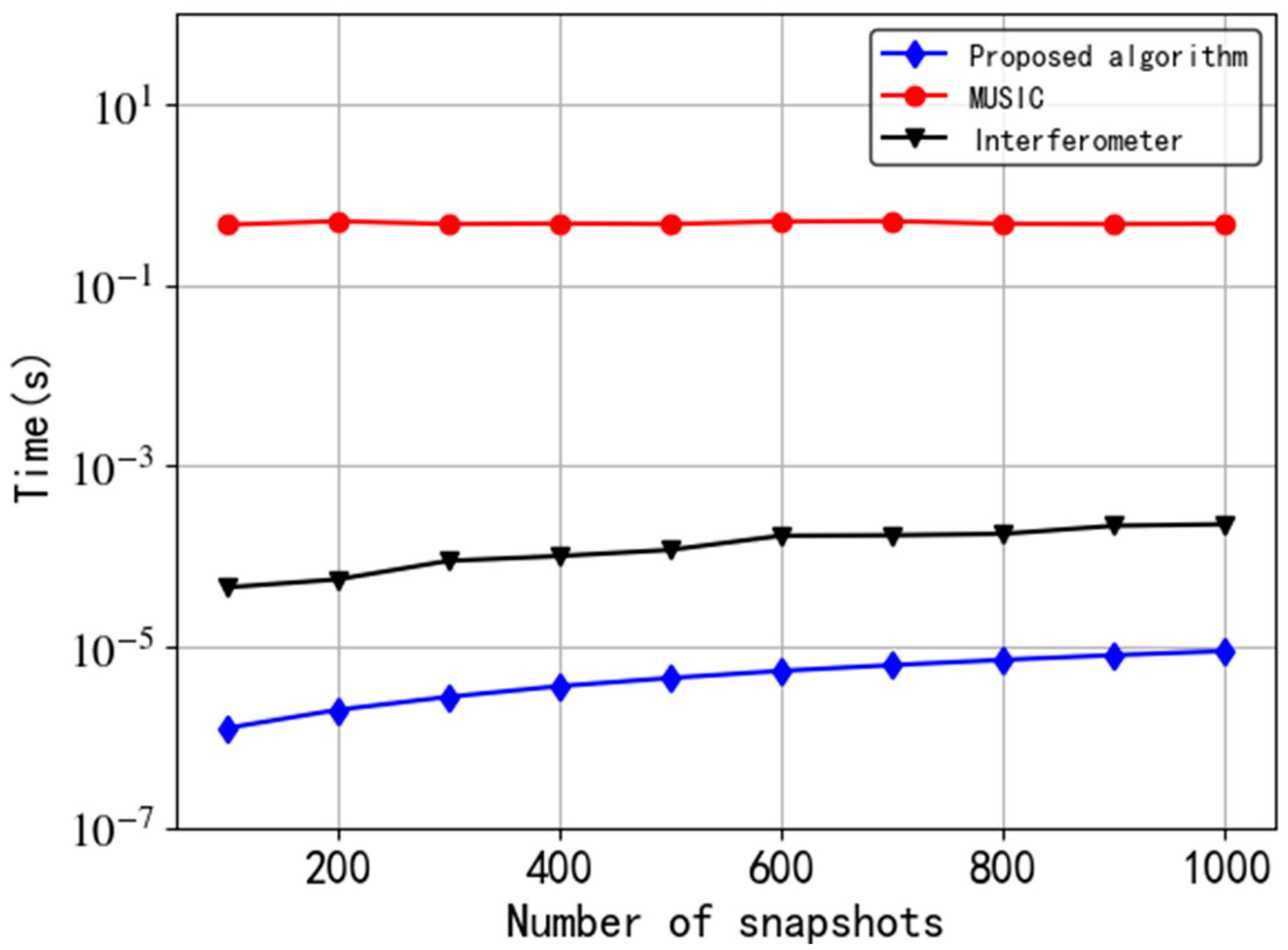
5.5. Simulation 5: Algorithm Complexity
In this simulation, we record the running time of different algorithms in MATLAB, which is obtained by taking the average of the running time of multiple Monte Carlo experiments. The version of MATLAB is 2018b. The CPU of the computer running the experiment is i7-7700HQ with a clock frequency of 2.8 GHz. The simulation results are shown in
Figure 8.
Figure 8 presents that the speed of the proposed algorithm and the interferometer algorithm are both much faster than that of the MUSIC algorithm. In detail, the running time of our algorithm is at least 5 orders of magnitude lower than that of MUSIC algorithm. Furthermore, as the number of snapshots increases, the calculation time of the interferometer algorithm is approximately 40 to 200 times that of the proposed algorithm. Obviously, the significant advantage of the proposed tripole antenna algorithm is the low computational complexity.


