Particle Filtering for Three-Dimensional TDoA-Based Positioning Using Four Anchor Nodes


Abstract
1. Introduction
2. Indoor Positioning of Unmanned Air Vehicles (UAVs)
3. Particle Filtering for TDoA-Based Positioning
3.1. Problem Statement and Concept of Solution
3.2. The Particle Filter
3.3. Particle Filter Implementation
| Algorithm 1 The particle filter algorithm. |
| 0. Initialization: Generate particles uniformly distributed in the whole working space. Compute the weight of each particle according to Equation (11), when TDoA measurements are available at time , . Estimate the position of the target node, , according to Equation (14). 1. Prediction: Generate new particles according to Equation (15). 2. Update: Compute the weight of each particle according to Equation (11), when TDoA measurements are available at time , . 3. State Estimation: Estimate the position of the target node, , according to Equation (14). Set and repeat from step 1. |
4. Simulation Results
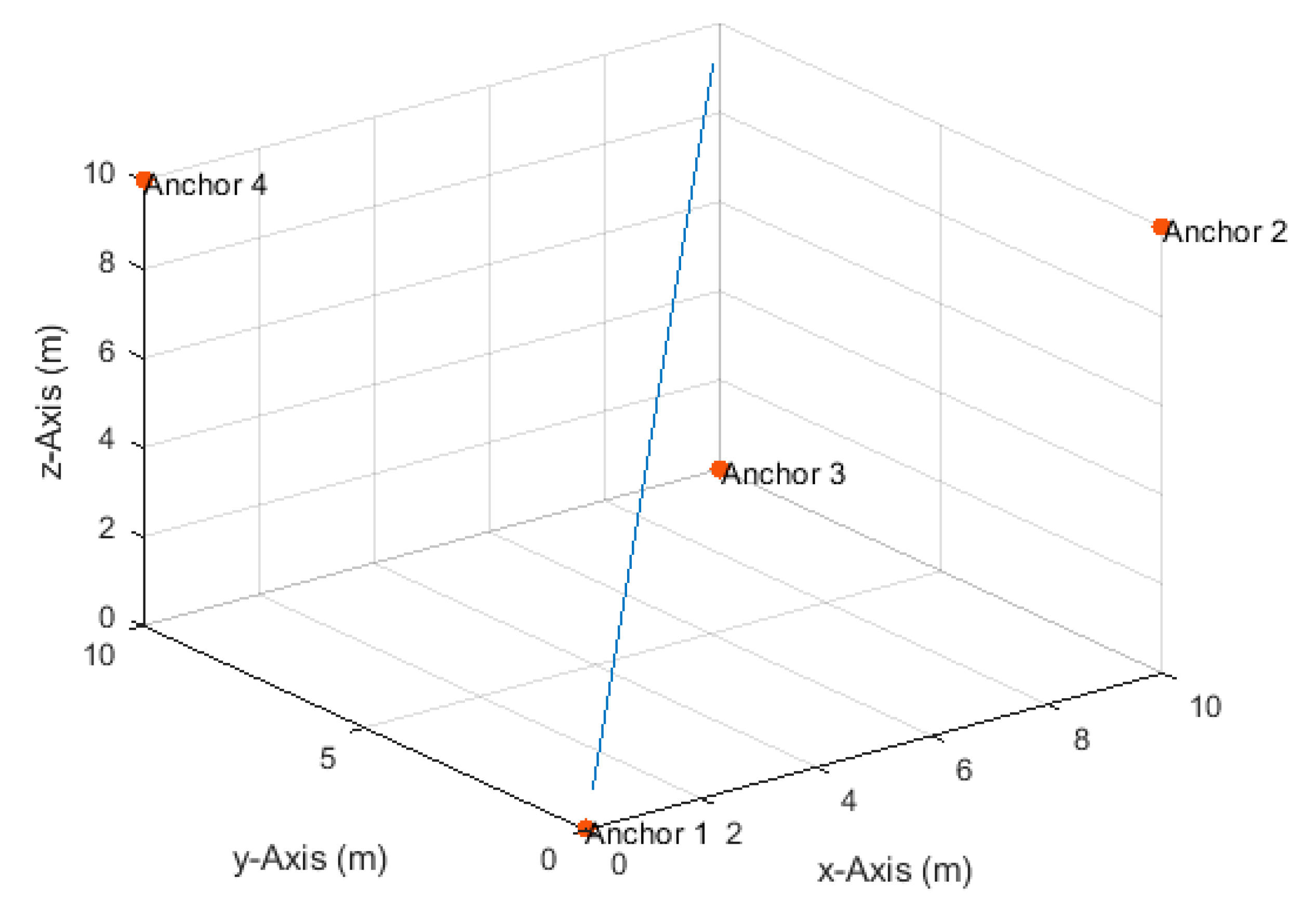
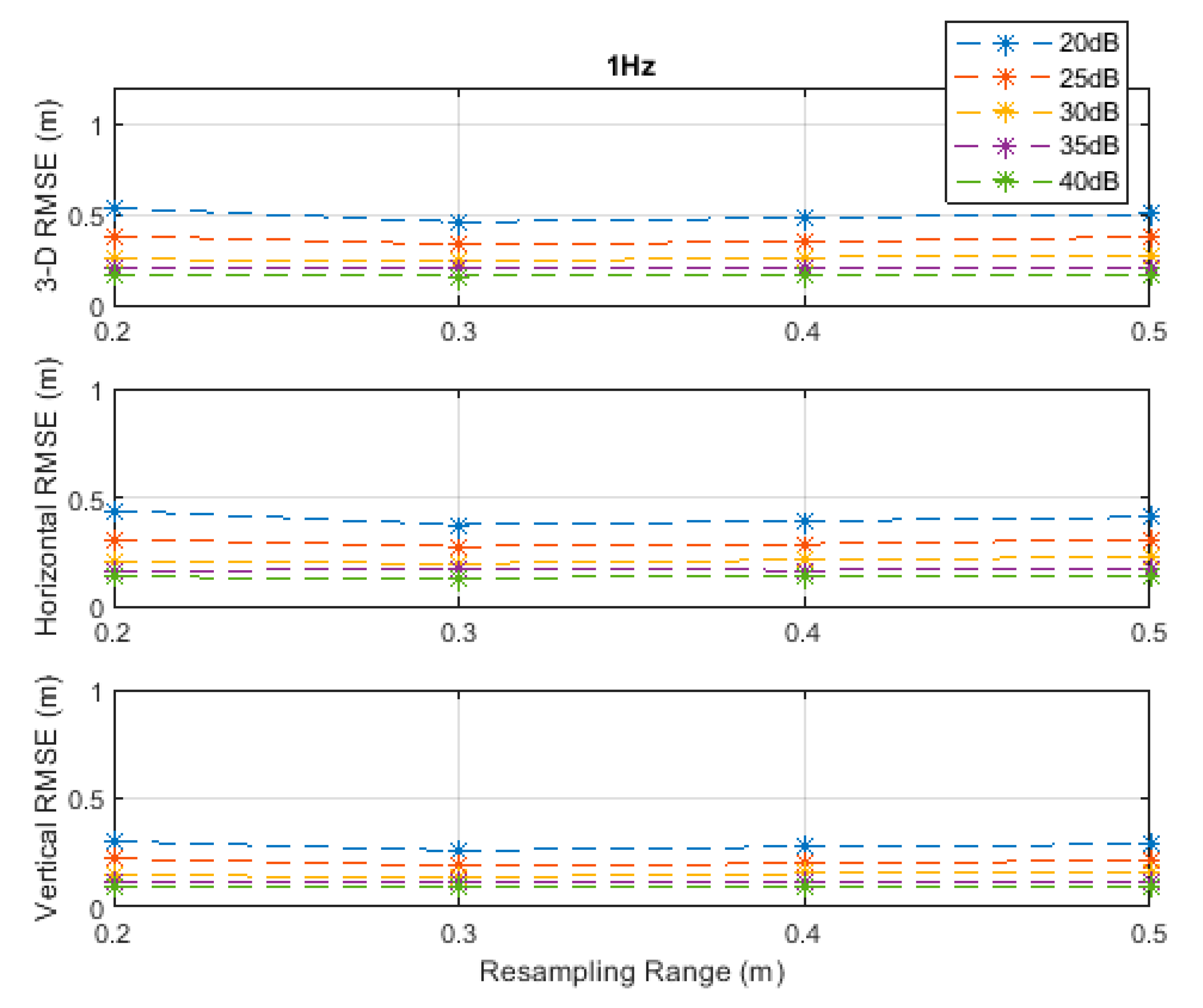
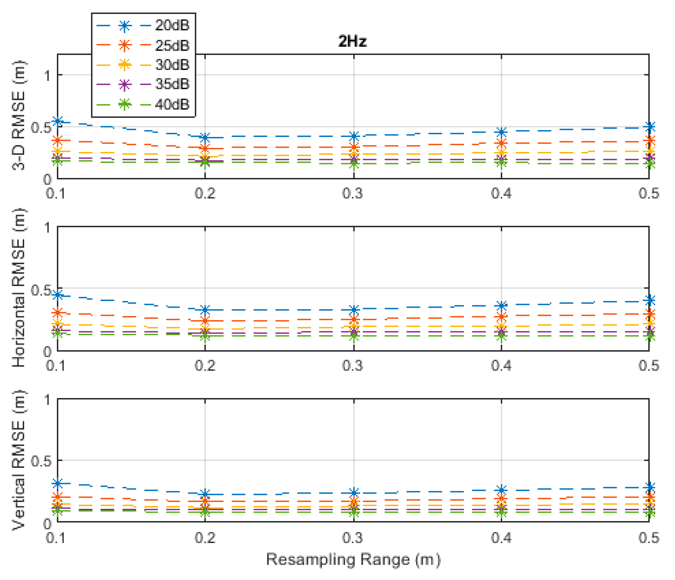
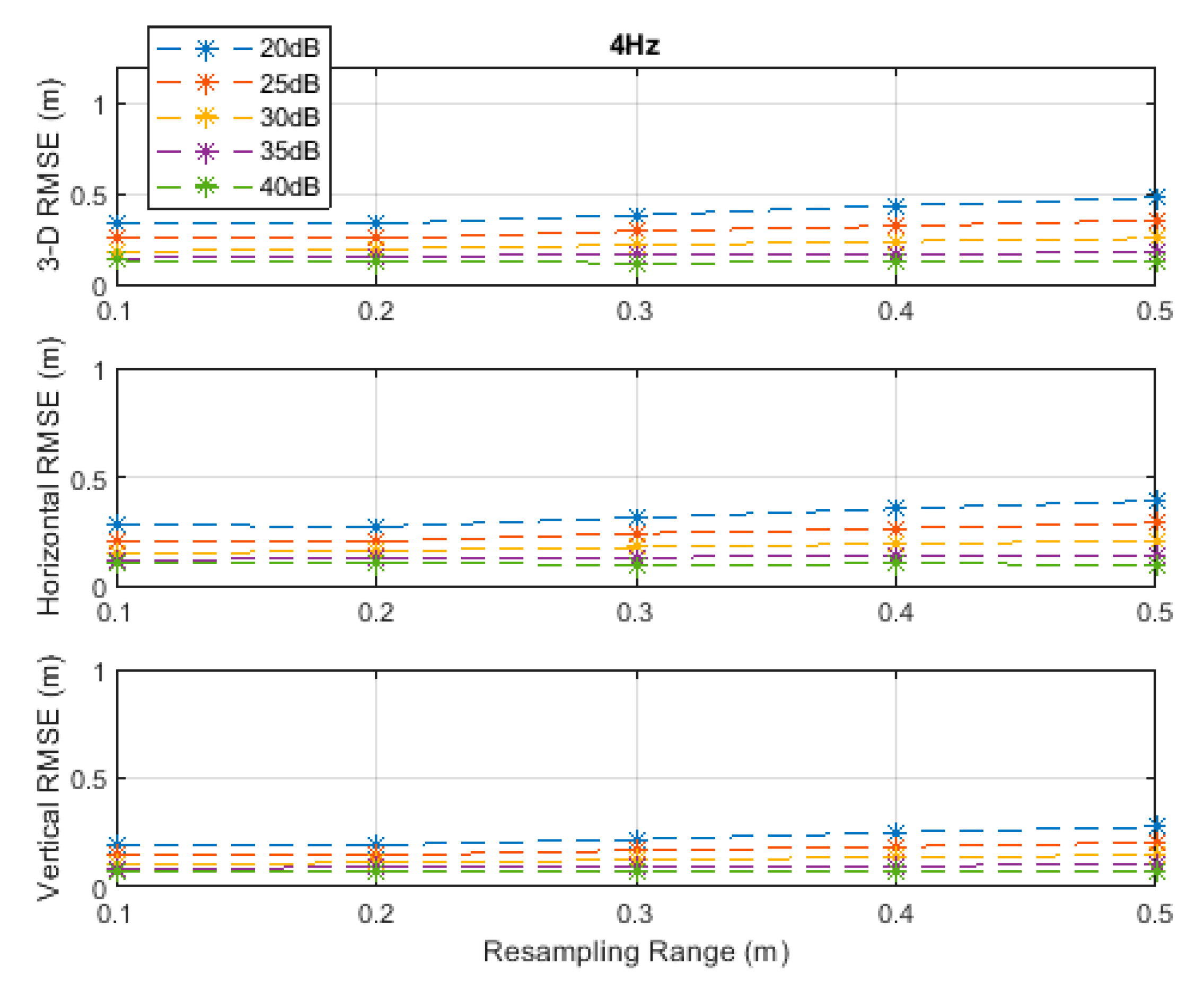
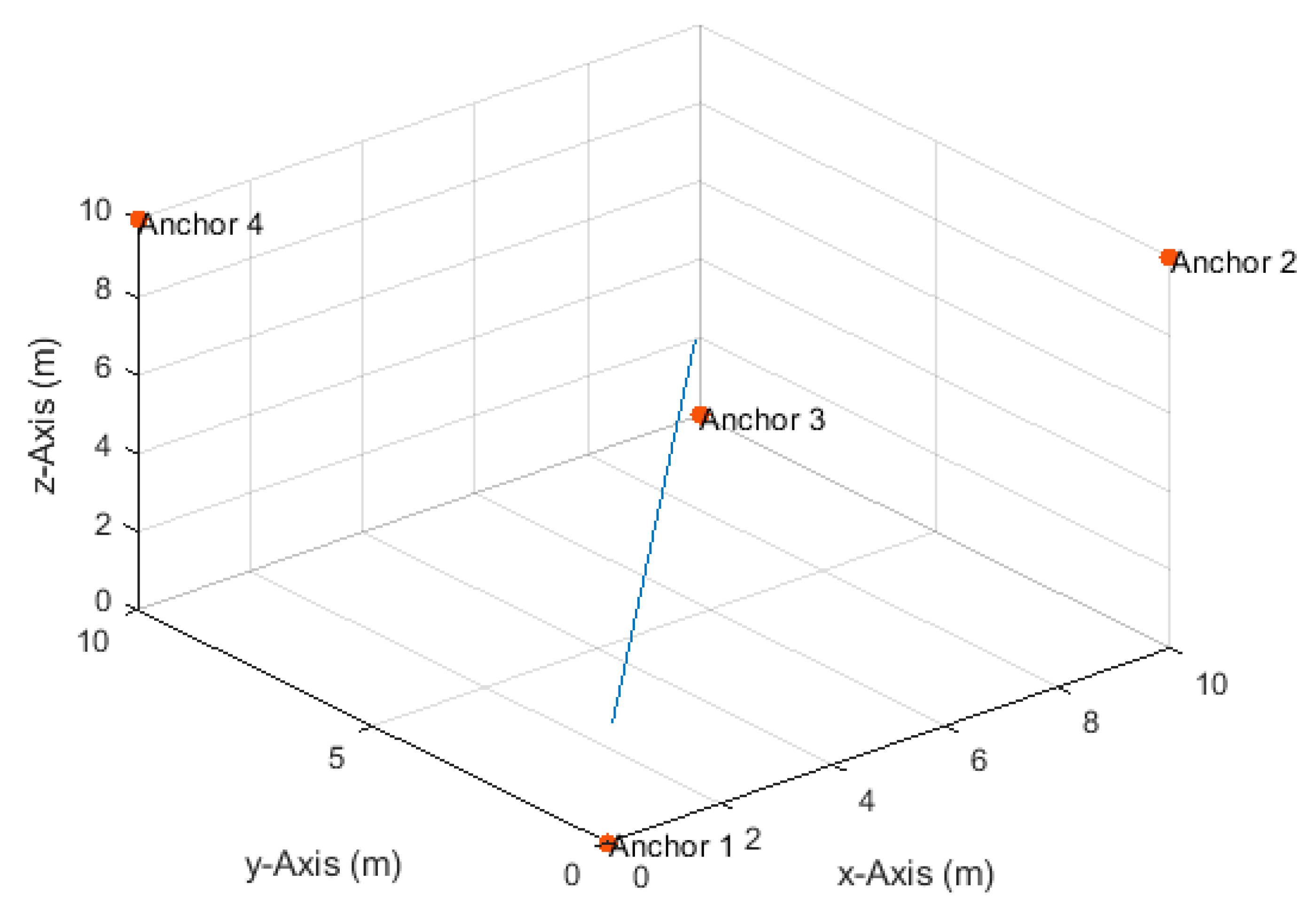
4.1. Three-Dimensional Linear Path
4.2. Horizontal Linear Path
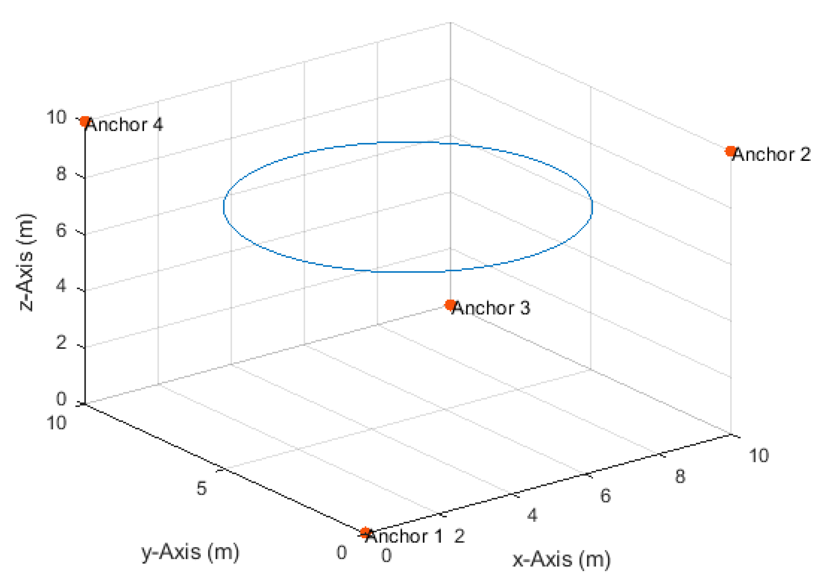
4.3. Horizontal Circular Path
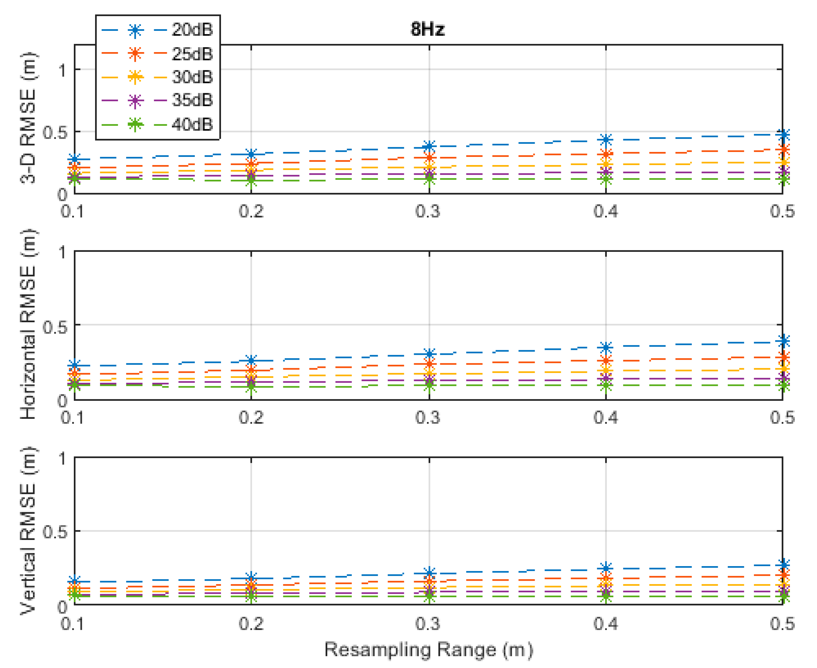
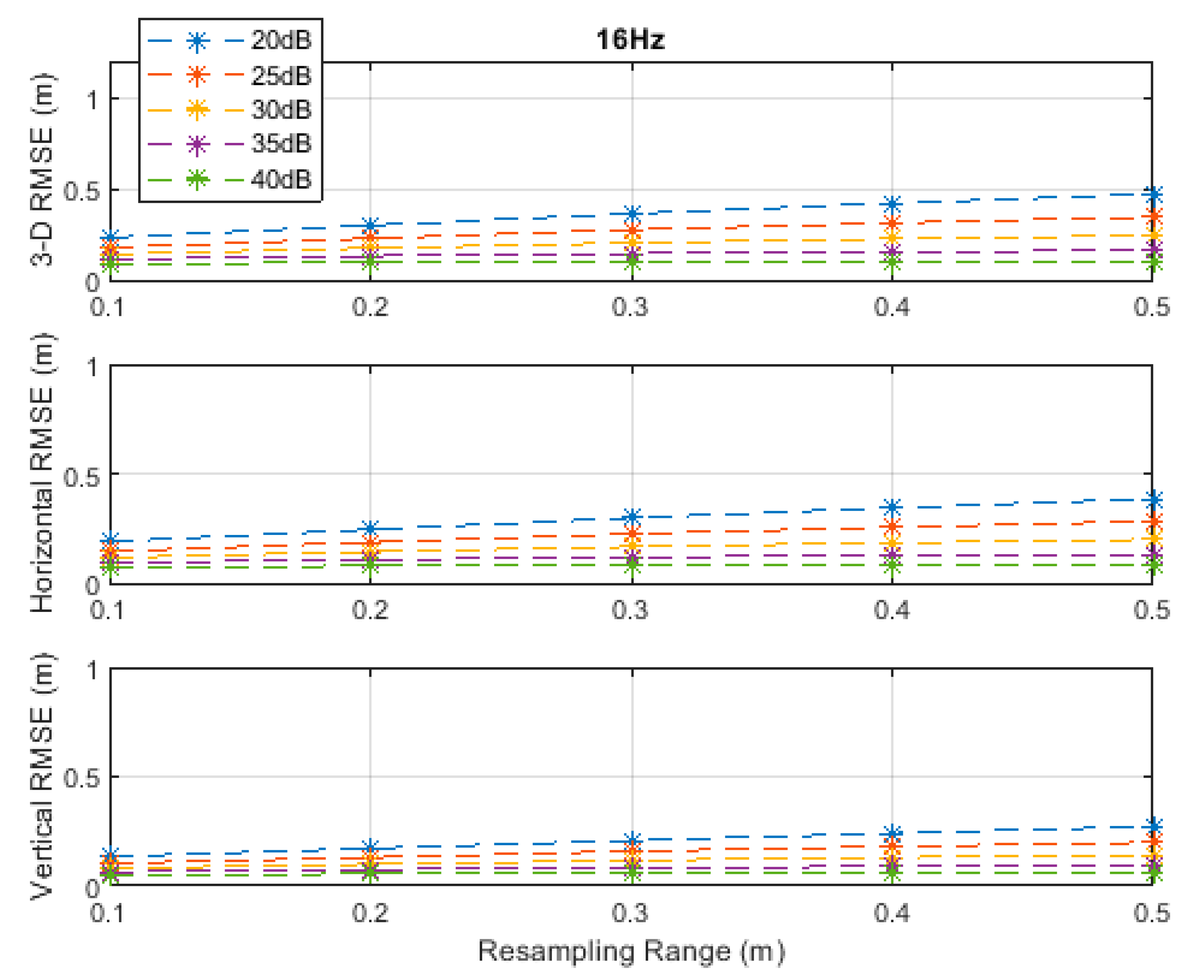
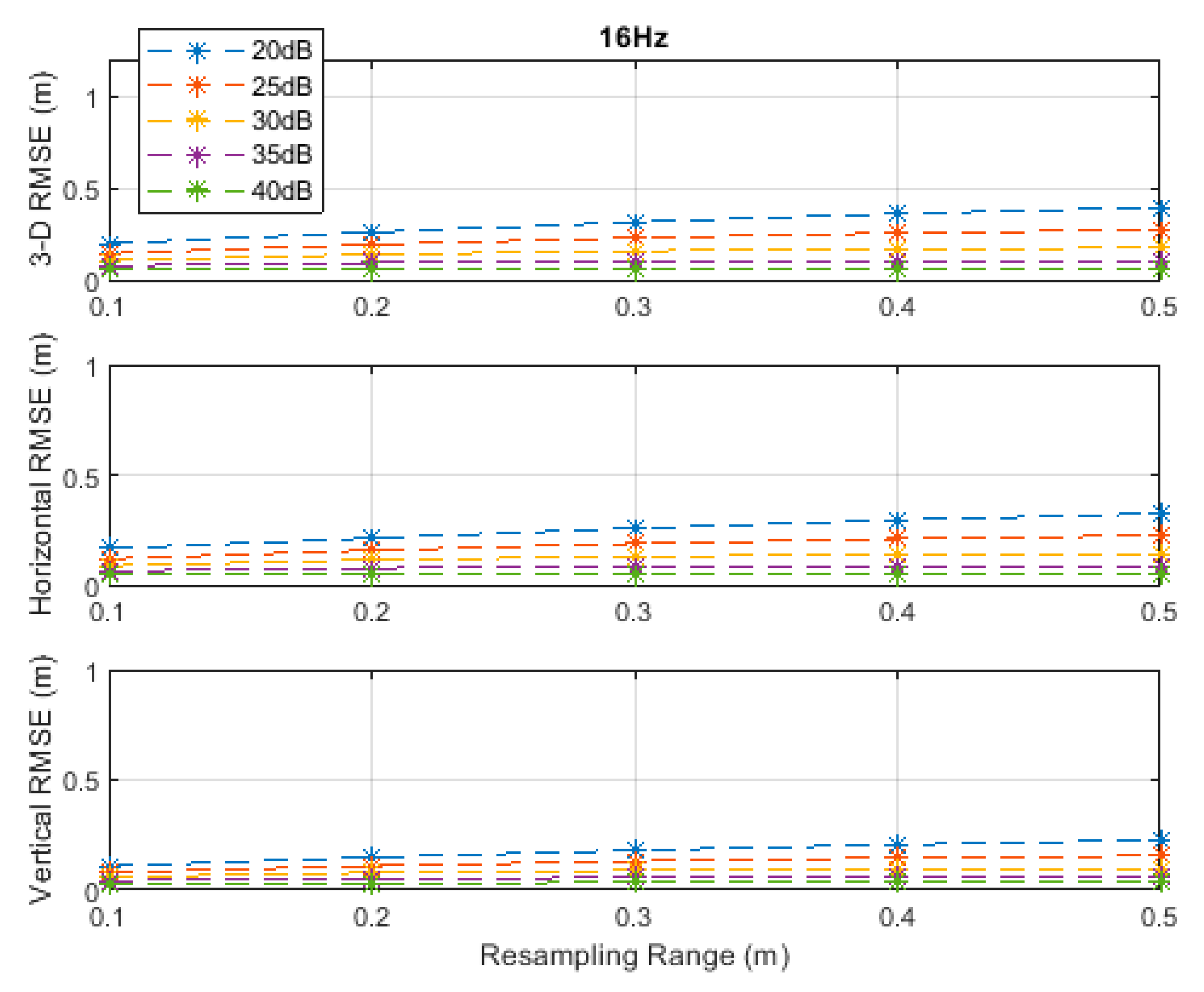
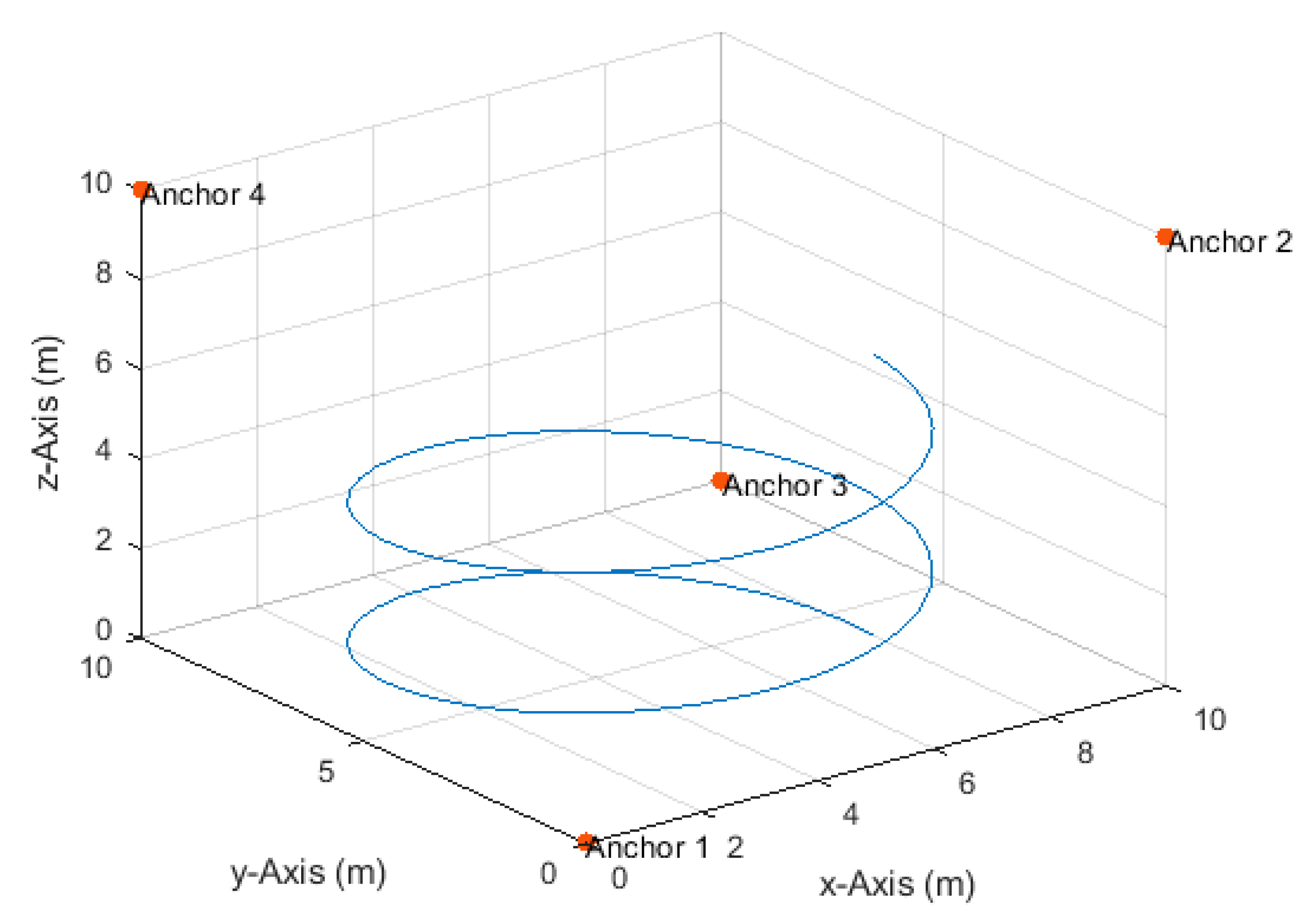
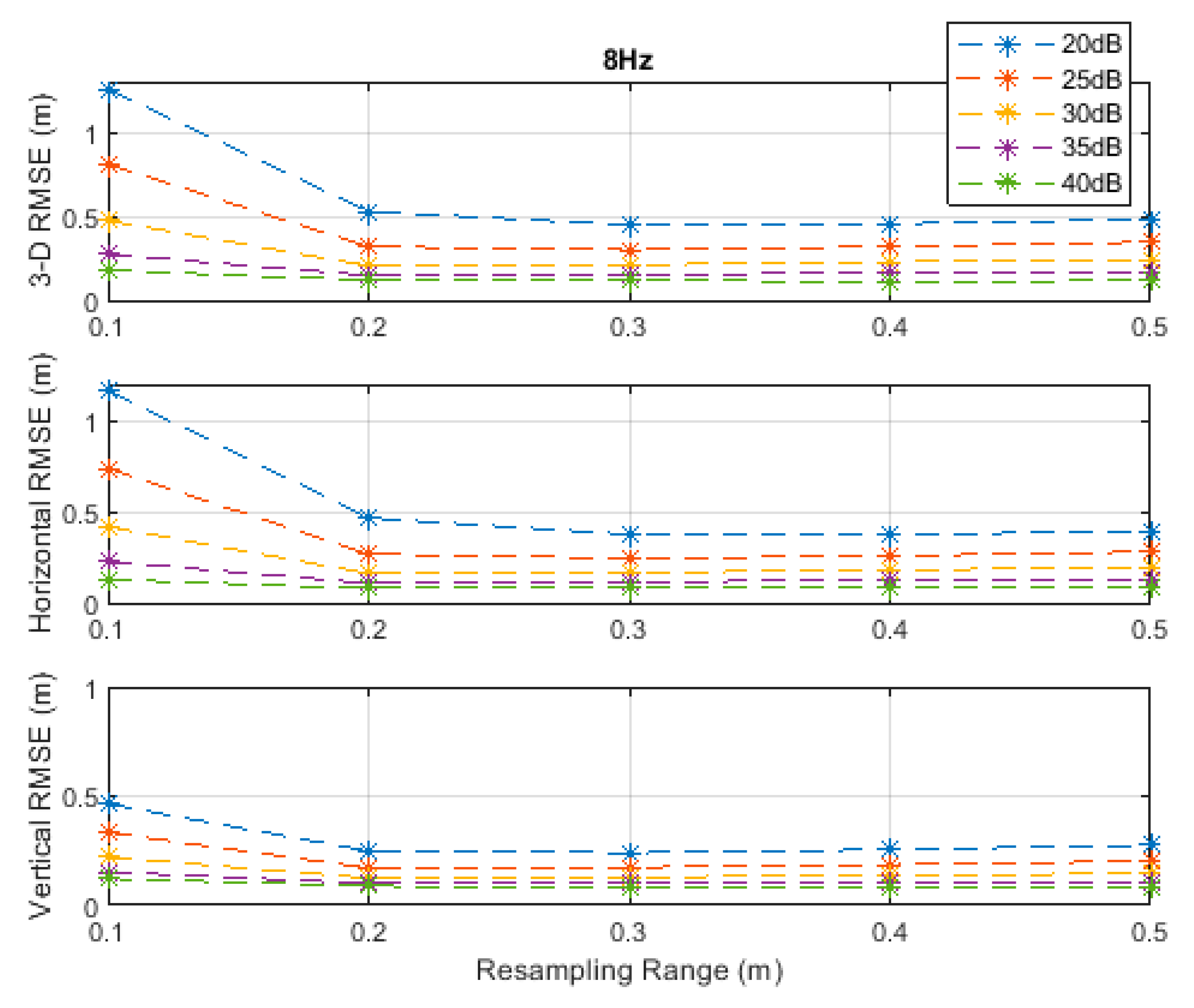
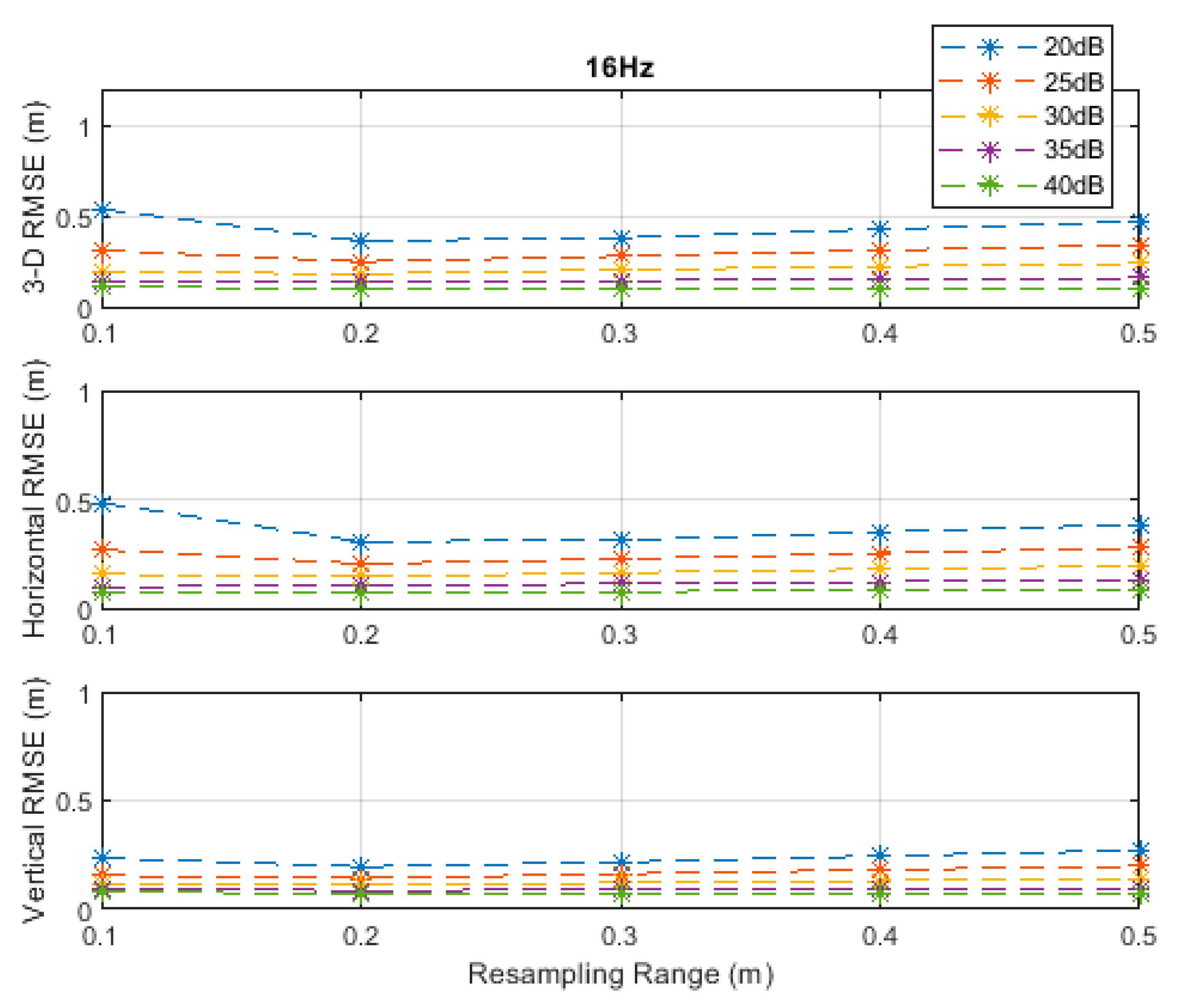
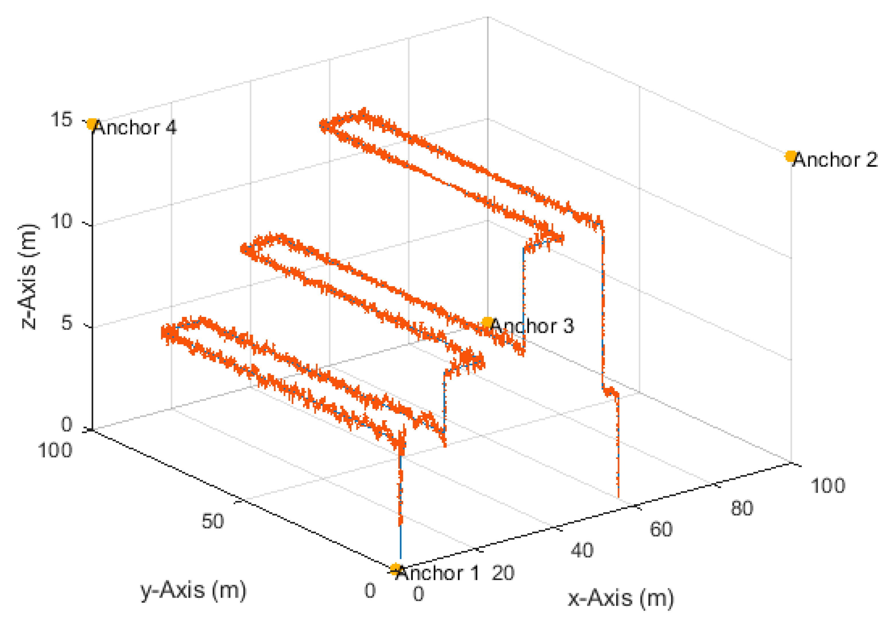
4.4. Helical Path
4.5. An Inventory Management Scenario
5. Conclusions
Funding
Acknowledgments
Conflicts of Interest
Abbreviations
| 2-D | Two-dimensional |
| 3-D | Three-dimensional |
| AUV | Autonomous underwater vehicles |
| EKF | Extended Kalman filter |
| GDOP | Geometric dilution of precision |
| GNSS | Global navigation satellite system |
| IMU | Inertial measurement unit |
| INS | Inertial navigation system |
| IoV | Internet of vehicles |
| KF | Kalman filter |
| LBS | Location-based services |
| LoS | Line-of-sight |
| MAV | Micro aerial vehicle |
| MCL | Monte Carlo localization |
| NLoS | Non-line-of-sight |
| Probability density function | |
| RF | Radiofrequency |
| RMSE | Root-mean-square error |
| SIR | Sample–importance–resample, sequential importance resampling |
| SMC | Sequential Monte Carlo |
| SNR | Signal-to-noise ratio |
| TDoA | Time difference of arrival |
| ToA | Time of arrival |
| ToF | Time of flight |
| UAV | Unmanned air vehicle |
| UKF | Unscented Kalman filter |
| UWB | Ultra-wide band |
| VLC | Visible light communications |
| WTAE | Weighted trimmed average estimate |
References
- Smith, J.O.; Abel, J.S. Closed-form least-squares source location estimation from range-difference measurements. IEEE Trans. Acoust. Speech Signal Process. 1987, 35, 1661–1669. [Google Scholar] [CrossRef]
- Chan, Y.T.; Ho, K.C. Simple and efficient estimator for hyperbolic location. IEEE Trans. Signal Process. 1994, 42, 1905–1915. [Google Scholar] [CrossRef]
- Dogancay, K.; Hashemi-Sakhtsari, A. Target tracking by time difference of arrival using recursive smoothing. Signal Process. 2005, 85, 667–679. [Google Scholar] [CrossRef]
- Xiao, W.; Weng, Y.; Xie, L. Total least squares method for robust source localization in sensor networks using TDOA measurements. Int. J. Distrib. Sens. Netw. 2011, 7, 172902. [Google Scholar]
- Lin, L.; So, H.C.; Chan, F.K.W.; Chan, Y.T.; Ho, K.C. A new constrained weighted least squares algorithm for TDOA-based localization. Signal Process. 2013, 93, 2872–2878. [Google Scholar] [CrossRef]
- Khalaf-Allah, M. An extended closed-form least-squares solution for three-dimensional hyperbolic geolocation. In Proceedings of the 2014 IEEE Symposium on Industrial Electronics Applications (ISIEA), Kota Kinabalu, Malaysia, 28 September–1 October 2014; pp. 7–11. [Google Scholar]
- Khalaf-Allah, M. Performance Comparison of Closed-Form Least Squares Algorithms for Hyperbolic 3-D Positioning. J. Sens. Actuator Netw. 2020, 9, 2. [Google Scholar] [CrossRef]
- Lui, K.W.; Chan, F.K.; So, H.C. Semidefinite programming approach for range-difference based source localization. IEEE Trans. Signal Process. 2009, 57, 1630–1633. [Google Scholar] [CrossRef]
- Li, T.; Ekpenyong, A.; Huang, Y.-F. Source localization and tracking using distributed asynchronous sensors. IEEE Trans. Signal Process. 2006, 54, 3991–4003. [Google Scholar] [CrossRef]
- Win, M.Z.; Conti, A.; Mazuelas, S.; Shen, Y.; Gifford, W.M.; Dardari, D.; Chiani, M. Network localization and navigation via cooperation. IEEE Commun. Mag. 2011, 49, 56–62. [Google Scholar] [CrossRef]
- Gholami, M.R.; Gezici, S.; Strom, E.G. Improved position estimation using hybrid TW-TOA and TDOA in cooperative networks. IEEE Trans. Signal Process. 2012, 60, 3770–3785. [Google Scholar] [CrossRef]
- Cakir, O.; Kaya, I.; Yazgan, A. Propagation speed free emitter location finding using TDOA. In Proceedings of the 21st Telecommunications Forum (TELFOR ’13), Belgrade, Serbia, 26 November 2013; pp. 405–407. [Google Scholar]
- De Sanctis, G.; Rovetta, D.; Sarti, A.; Scarparo, G.; Tubaro, S. Localization of tactile interactions through TDOA analysis: Geometric vs. inversion-based method. In Proceedings of the 14th European Signal Processing Conference (EUSIPCO ’06), Florence, Italy, 4 September 2006. [Google Scholar]
- Chen, J.C.; Yao, K.; Hudson, R.E. Source localization and beamforming. IEEE Signal Process. Mag. 2002, 19, 30–39. [Google Scholar] [CrossRef]
- Priyantha, N.B.; Balakrishnan, H.; Demaine, E.D.; Teller, S. Mobile-assisted localization in wireless sensor networks. In Proceedings of the IEEE 24th Annual Joint Conference of the IEEE Computer and Communications Societies, Miami, FL, USA, 13–17 March 2005. [Google Scholar]
- Díez-González, J.; Álvarez, R.; Sánchez-González, L.; Fernández-Robles, L.; Pérez, H.; Castejón-Limas, M. 3D Tdoa Problem Solution with Four Receiving Nodes. Sensors 2019, 19, 2892. [Google Scholar] [CrossRef] [PubMed]
- Nonami, K. Prospect and recent research & development for civil use autonomous unmanned aircraft as UAV and MAV. J. Syst. Design Dyn. 2007, 1, 120–128. [Google Scholar]
- Tomic, T.; Schmid, K.; Lutz, P.; Domel, A.; Kassecker, M.; Mair, E.; Grixa, I.L.; Ruess, F.; Suppa, M.; Burschka, D. Toward a fully autonomous UAV: Research platform for indoor and outdoor urban search and rescue. IEEE Robot. Autom. Mag. 2012, 19, 46–56. [Google Scholar] [CrossRef]
- López, L.B.; van Manen, N.; van der Zee, E.; Bos, S. DroneAlert: Autonomous Drones for Emergency Response. In Multi-Technology Positioning, 2nd ed.; Nurmi, J., Lohan, E.-S., Wymeersch, H., Seco-Granados, G., Nykänen, O., Eds.; Springer International Publishing AG: Cham, Switzerland, 2017; pp. 303–321. [Google Scholar]
- Xu, Y.; Choi, J.; Dass, S.; Maiti, T. Bayesian Prediction and Adaptive Sampling Algorithms for Mobile Sensor Networks, 3rd ed.; Springer: Cham, Switzerland, 2017; pp. 1–6. [Google Scholar]
- Sukhatme, G.S.; Dhariwal, A.; Zhang, B.; Oberg, C.; Stauffer, B.; Caron, D.A. Design and development of a wireless robotic networked aquatic microbial observing system. Environ. Eng. Sci. 2007, 24, 205–215. [Google Scholar] [CrossRef]
- Wang, Y.; Tan, R.; Xing, G.; Tan, X.; Wang, J.; Zhou, R. Spatiotemporal aquatic field reconstruction using cyber-physical robotic sensor systems. ACM Trans. Sensor Netw. (TOSN) 2014, 10, 1–27. [Google Scholar] [CrossRef]
- Laut, J.; Henry, E.; Nov, O.; Porfiri, M. Development of a mechatronics-based citizen science platform for aquatic environmental monitoring. IEEE Trans. Mechatron. 2014, 19, 1541–1551. [Google Scholar] [CrossRef]
- Choi, J.; Milutinovic, D. Tips on stochastic optimal feedback control and Bayesian spatiotemporal models: Applications to robotics. J. Dyn. Syst. Meas. Control. 2015, 137. [Google Scholar] [CrossRef]
- Mupparapu, S.S.; Chappell, S.G.; Komerska, R.J.; Blidberg, D.R.; Nitzel, R.; Benton, C.; Popa, D.O.; Sanderson, A.C. Autonomous systems monitoring and control (ASMAC)—An AUV fleet controller. In Proceedings of the 2004 IEEE/OES Autonomous Underwater Vehicles, Sebasco, ME, USA, 17–18 June 2004; pp. 119–126. [Google Scholar]
- Nickell, C.L.; Woolsey, C.A.; Stilwell, D.J. A low-speed control module for a stream lined AUV. In Proceedings of the OCEANS 2005 MTS/IEEE, Washington, DC, USA, 17–23 September 2005; pp. 1680–1685. [Google Scholar]
- Bandyopadhyay, P.R. Trends in biorobotic autonomous undersea vehicles. IEEE J. Ocean. Eng. 2005, 30, 109–139. [Google Scholar] [CrossRef]
- Liu, Y.; Shen, Y. UAV-Aided High-Accuracy Relative Localization of Ground Vehicles. In Proceedings of the IEEE International Conference on Communications (ICC), Kansas City, MO, USA, 20–24 May 2018. [Google Scholar]
- Zeng, Y.; Zhang, R.; Lim, T.J. Wireless communications with unmanned aerial vehicles: Opportunities and challenges. IEEE Commun. Mag. 2016, 54, 36–42. [Google Scholar] [CrossRef]
- Matolak, D.W.; Sun, R. Unmanned aircraft systems: Air-ground channel characterization for future applications. IEEE Veh. Technol. Mag. 2015, 10, 79–85. [Google Scholar] [CrossRef]
- Mario, G.; Eun-Kyu, L.; Giovanni, P.; Uichin, L. Internet of vehicles: From intelligent grid to autonomous cars and vehicular clouds. In Proceedings of the 2016 IEEE 3rd World Forum on Internet of Things (WF-IoT), Reston, VA, USA, 12–14 December 2016; pp. 241–246. [Google Scholar]
- Pérez, M.C.; Gualda, D.; Vicente, J.; Villadangos, J.M.; Ureña, J. Review of UAV positioning in indoor environments and new proposal based on US measurements. In Proceedings of the 10th International Conference on Indoor Positioning and Indoor Navigation—Work-in-Progress (IPIN-WiP) Papers, Pisa, Italy, 30 September–3 October 2019; pp. 267–274. [Google Scholar]
- De Croon, G.; De Wagter, C. Challenges of Autonomous Flight in Indoor Environments. In Proceedings of the 2018 IEEE/RSJ International Conference on Intelligent Robots and Systems (IROS), Madrid, Spain, 1–5 October 2018. [Google Scholar]
- Bristeau, P.-J.; Callou, F.; Vissiere, D.; Petit, N. The navigation and control technology inside the AR.Drone micro uav. IFAC Proc. 2011, 44, 1477–1484. [Google Scholar] [CrossRef]
- Leutenegger, S.; Lynen, S.; Bosse, M.; Siegwart, R.; Furgale, P. Keyframe-based visual–inertial odometry using nonlinear optimization. Int. J. Robot. Res. 2015, 34, 314–334. [Google Scholar] [CrossRef]
- Tanskanen, P.; Naegeli, T.; Pollefeys, M.; Hilliges, O. Semi-direct ekf-based monocular visual-inertial odometry. In Proceedings of the 2015 IEEE/RSJ International Conference on Intelligent Robots and Systems (IROS), Hamburg, Germany, 28 September–2 October 2015; pp. 6073–6078. [Google Scholar]
- Balamurugan, G.; Valarmathi, J.; Naidu, V.P.S. Survey on UAV Navigation in GPS Denied Environments. In Proceedings of the 2016 International Conference on Signal Processing, Communication, Power and Embedded System, Paralakhemundi, India, 3–5 October 2016; pp. 198–204. [Google Scholar]
- Shang, C.; Cheng, L.; Yu, Q.; Wang, X.; Peng, R. Micro Aerial Vehicle Autonomous Flight Control in Tunnel Environment. In Proceedings of the 9th International Conference on Modelling, Identification and Control (ICMIC), Kunming, China, 10–12 July 2017. [Google Scholar]
- Paredes, J.A.; Álvarez, F.J.; Aguilera, T.; Villadangos, J.M. 3D Indoor positioning of UAVs with spread spectrum ultrasound and Time-of-Flight Cameras. Sensors 2018, 18, 89. [Google Scholar] [CrossRef]
- Ashok, A. Position: DroneVLC: Visible Light Communication for Aerial Vehicular Networking. In Proceedings of the 4th ACM Workshop on Visible Light Communication Systems (VLCS), Snowbird, UT, USA, 16 October 2017; pp. 29–30. Available online: https://dl.acm.org/doi/abs/10.1145/3129881.3129894 (accessed on 12 August 2020).
- Opromolla, R.; Fasano, G.; Rufino, G.; Grassi, M.; Savvaris, A. LIDAR-Inertial Integration for UAV Localization and Mapping in Complex Environments. In Proceedings of the 2016 International Conference on Unmanned Aircraft Systems (ICUAS), Arlington, VA, USA, 7–10 June 2016. [Google Scholar]
- Guerra, E.; Munguía, R.; Grau, A. UAV Visual and Laser Sensor Fusion for Detection and Positioning in Industrial Applications. Sensors 2018, 18, 2071. [Google Scholar] [CrossRef]
- Tiemann, J.; Wietfeld, C. Scalable and Precise Multi-UAV Indoor Navigation using TDOA-based UWB Localization. In Proceedings of the 2017 International Conference on Indoor Positioning and Indoor Navigation (IPIN), Sapporo, Japan, 18–21 September 2017. [Google Scholar]
- Perez-Grau, F.J.; Caballero, F.; Merino, L.; Viguria, A. Multi-modal Mapping and Localization of Unmanned Aerial Robots based on Ultra-Wideband and RGB-D sensing. In Proceedings of the 2017 IEEE/RSJ International Conference on Intelligent Robots and Systems (IROS), Vancouver, BC, Canada, 24–28 September 2017. [Google Scholar]
- Li, J.; Bi, Y.; Li, K.; Wang, K.; Lin, F.; Chen, B.M. Accurate 3D Localization for MAV Swarms by UWB and IMU Fusion. In Proceedings of the 2018 IEEE 14th International Conference on Control and Automation (ICCA), Anchorage, AK, USA, 12–15 June 2018. [Google Scholar]
- Yan, J.; Yang, X.; Ye, H.; Wang, Z. Integrated Positioning and Obstacle Avoidance for Multi-Quadrotors in an Indoor Office Environment. In Proceedings of the 38th Chinese Control Conference, Guangzhou, China, 27–30 July 2019. [Google Scholar]
- Macoir, N.; Bauwens, J.; Jooris, B.; Van Herbruggen, B.; Rossey, J.; Hoebeke, J.; De Poorter, E. UWB Localization with Battery-Powered Wireless Backbone for Drone-Based Inventory Management. Sensors 2019, 19, 467. [Google Scholar] [CrossRef]
- Kwon, W.; Park, J.H.; Lee, M.; Her, J.; Kim, S.-H.; Seo, J.-W. Robust Autonomous Navigation of Unmanned Aerial Vehicles (UAVs) for Warehouses’ Inventory Application. IEEE Robot. Autom. Lett. 2020, 5, 243–249. [Google Scholar] [CrossRef]
- Mashood, A.; Dirir, A.; Hussein, M.; Noura, H.; Awwad, F. Quadrotor object tracking using real-time motion sensing. In Proceedings of the 5th International Conference on Electronic Devices, Systems and Applications (ICEDSA), Ras Al Khaimah, United Arab, 6–8 December 2016. [Google Scholar]
- Beul, M.; Droeschel, D.; Nieuwenhuisen, M.; Quenzel, J.; Houben, S.; Behnke, S. Fast autonomous flight in warehouses for inventory applications. IEEE Robot. Autom. Lett. 2018, 3, 3121–3128. [Google Scholar] [CrossRef]
- Campos-Macias, L.; Aldana-López, R.; de la Guardia, R.; Parra-Vilchis, J.I.; Gómez-Gutiérrez, D. Autonomous Navigation of MAVs in Unknown Cluttered Environments. Available online: https://arxiv.org/abs/1906.08839 (accessed on 12 May 2020).
- Welburn, E.; Hakim Khalili, H.; Gupta, A.; Watson, S.; Carrasco, J. A navigational system for quadcopter remote inspection of offshore substations. In Proceedings of the 15th International Conference on Autonomic and Autonomous Systems (ICAS), Athens, Greece, 2–6 June 2019; pp. 32–37. [Google Scholar]
- Kalinov, I.; Safronov, E.; Agishev, R.; Kurenkov, M.; Tsetserukou, D. High-precision UAV localization system for landing on a mobile collaborative robot based on an IR marker pattern recognition. In Proceedings of the 2019 IEEE 89th Vehicular Technology Conference (VTC2019-Spring), Kuala Lumpur, Malaysia, 28 April–1 May 2019; pp. 1–6. [Google Scholar]
- Särkkä, S. Bayesian Filtering and Smoothing; Cambridge University Press: Cambridge, UK, 2013. [Google Scholar]
- Jazwinski, A.H. Stochastic Processes and Filtering Theory; Academic Press: New York, NY, USA, 1970. [Google Scholar]
- Gordon, N.J.; Salmond, D.J.; Smith, A.F.M. Novel approach to nonlinear/non-Gaussian Bayesian state estimation. IEE Proc. F 1993, 140, 107–113. [Google Scholar] [CrossRef]
- Arulampalam, S.; Maskell, S.; Gordon, N.; Clapp, T. A tutorial on particle filters for on-line non-linear/non-Gaussian Bayesian tracking. IEEE Trans. Signal Process. 2002, 50, 174–188. [Google Scholar] [CrossRef]
- Gustafsson, F.; Gunnarsson, F.; Bergman, N.; Forssell, U.; Jansson, J.; Karlsson, R.; Nordlund, P.J. Particle filters for positioning, navigation, and tracking. IEEE Trans. Signal Process. 2002, 50, 425–437. [Google Scholar] [CrossRef]
- Simon, D. Optimal State Estimation; Wiley: Hoboken, NJ, USA, 2006. [Google Scholar]
- Gustafsson, F. Particle filter theory and practice with positioning applications. IEEE Aerosp. Electron. Syst. Mag. 2010, 25, 53–82. [Google Scholar] [CrossRef]
- Del Moral, P. Nonlinear filtering using random particles. Theory Probab. Appl. 1996, 40, 690–701. [Google Scholar] [CrossRef]
- Hu, X.L.; Schon, T.B.; Ljung, L. A basic convergence result for particle filtering. IEEE Trans Signal Process. 2008, 56, 1337–1348. [Google Scholar] [CrossRef]
- Nordlund, P.J.; Gunnarsson, F.; Gustafsson, F. Particle filters for positioning in wireless networks. In Proceedings of the 11th European Signal Processing Conference (EUSIPCO), Toulouse, France, 3–6 September 2002. [Google Scholar]
- Li, H.; Wang, J.; Liu, Y. Passive coherent radar tracking algorithm based on particle filter and multiple TDOA measurements. In Proceedings of the 2nd International Congress on Image and Signal Processing (CISP), Tianjin, China, 17–19 October 2009. [Google Scholar]
- Boccadoro, M.; De Angelis, G.; Valigi, P. TDOA positioning in NLOS scenarios by particle filtering. Wirel. Netw. 2012, 18, 579–589. [Google Scholar] [CrossRef]
- Hol, J.D.; Schon, T.B.; Gustafsson, F. On resampling algorithms for particle filters. In Proceedings of the 2006 IEEE Nonlinear Statistical Signal Processing Workshop, Cambridge, UK, 13–15 September 2006. [Google Scholar]
- Li, T.; Bolic, M.; Djuric, P.M. Resampling methods for particle filtering: Classification, implementation, and strategies. IEEE Signal Process. Mag. 2015, 32, 70–86. [Google Scholar] [CrossRef]
- Turgut, B.; Martin, R.P. Restarting particle filters: An approach to improve the performance of dynamic indoor localization. In Proceedings of the 2009 IEEE Global Telecommunications Conference (GLOBECOM), Honolulu, HI, USA, 30 November–4 December 2009; pp. 1–7. [Google Scholar]
- Guo, K.; Qiu, Z.; Miao, C.; Zaini, A.H.; Chen, C.L.; Meng, W.; Xie, L. Ultra-Wideband-Based Localization for Quadcopter Navigation. Unmanned Syst. 2016, 4, 23–34. [Google Scholar] [CrossRef]
- Tzoreff, E.; Weiss, A.J. Expectation-maximization algorithm for direct position determination. Signal Process. 2017, 133, 32–39. [Google Scholar] [CrossRef]
- Ma, F.; Yang, L.; Zhang, M.; Guo, F.-C. TDOA source positioning in the presence of outliers. IET Signal Process. 2019, 13, 679–688. [Google Scholar] [CrossRef]


| Measurement Update Rate (Hz) | Total No. of Measurements | Traveled Distance (cm) |
|---|---|---|
| 1 | 91 | 10 |
| 2 | 181 | 5 |
| 4 | 361 | 2.5 |
| 8 | 721 | 1.25 |
| 16 | 1441 | 0.625 |
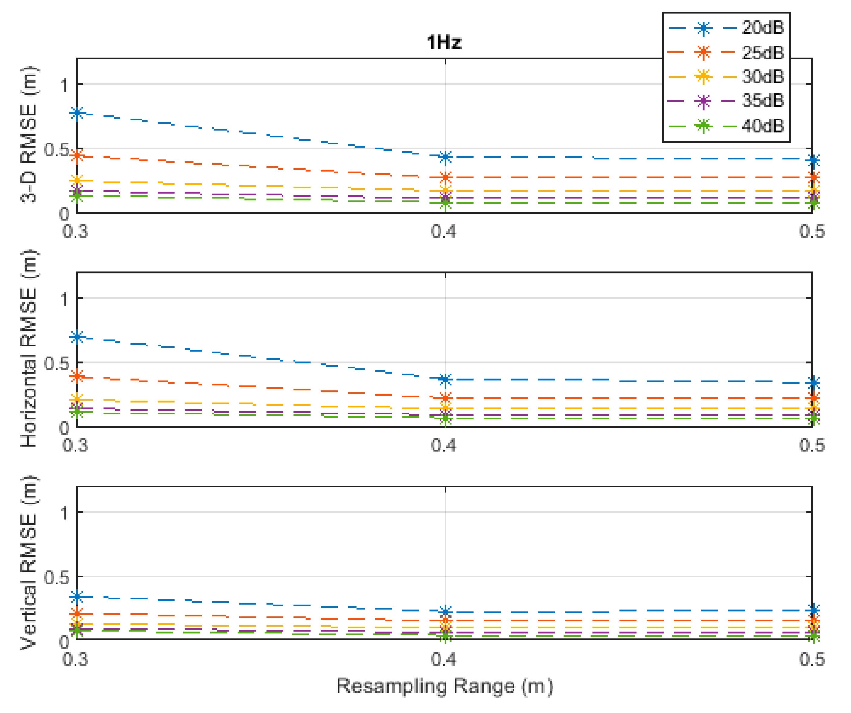
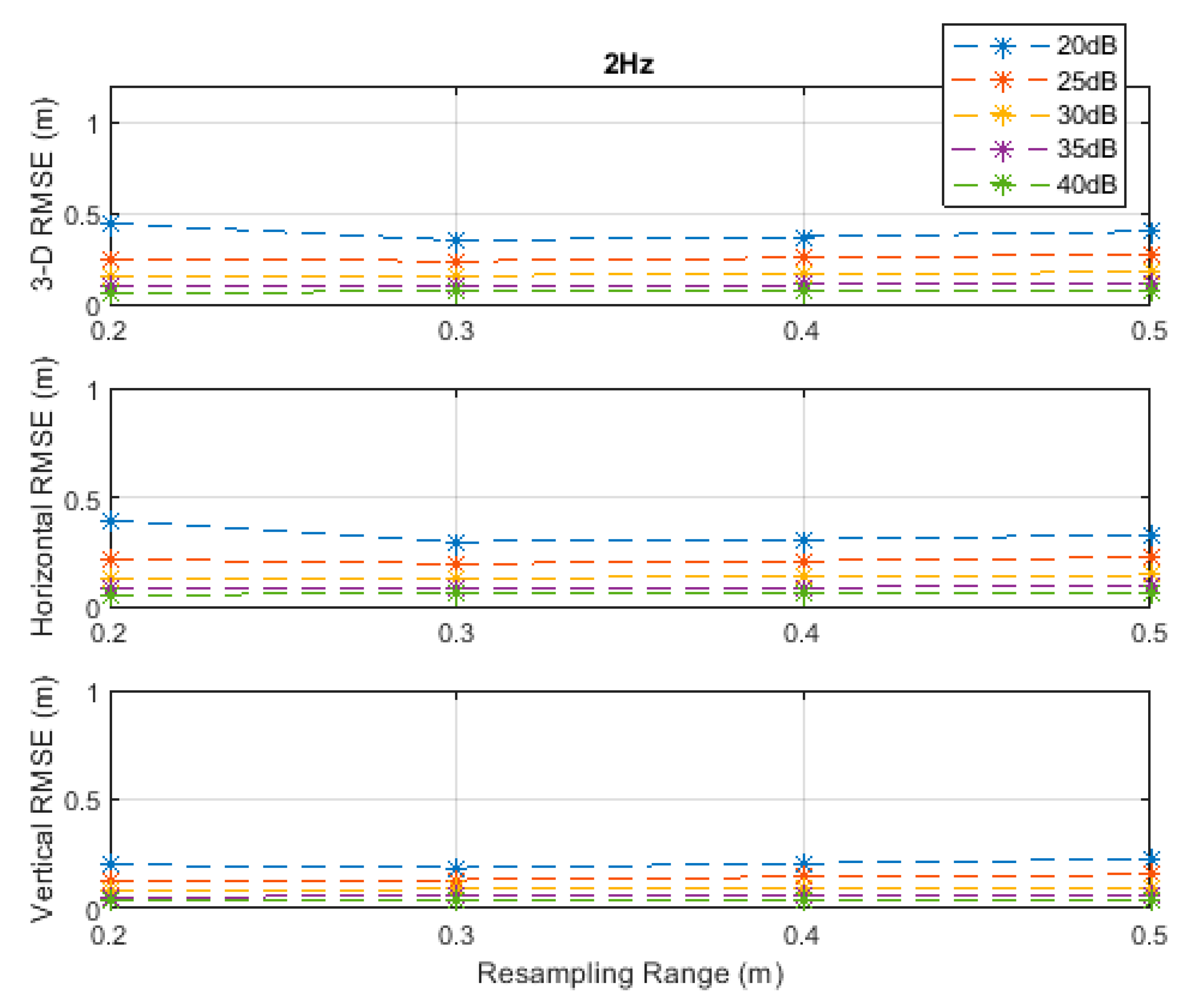
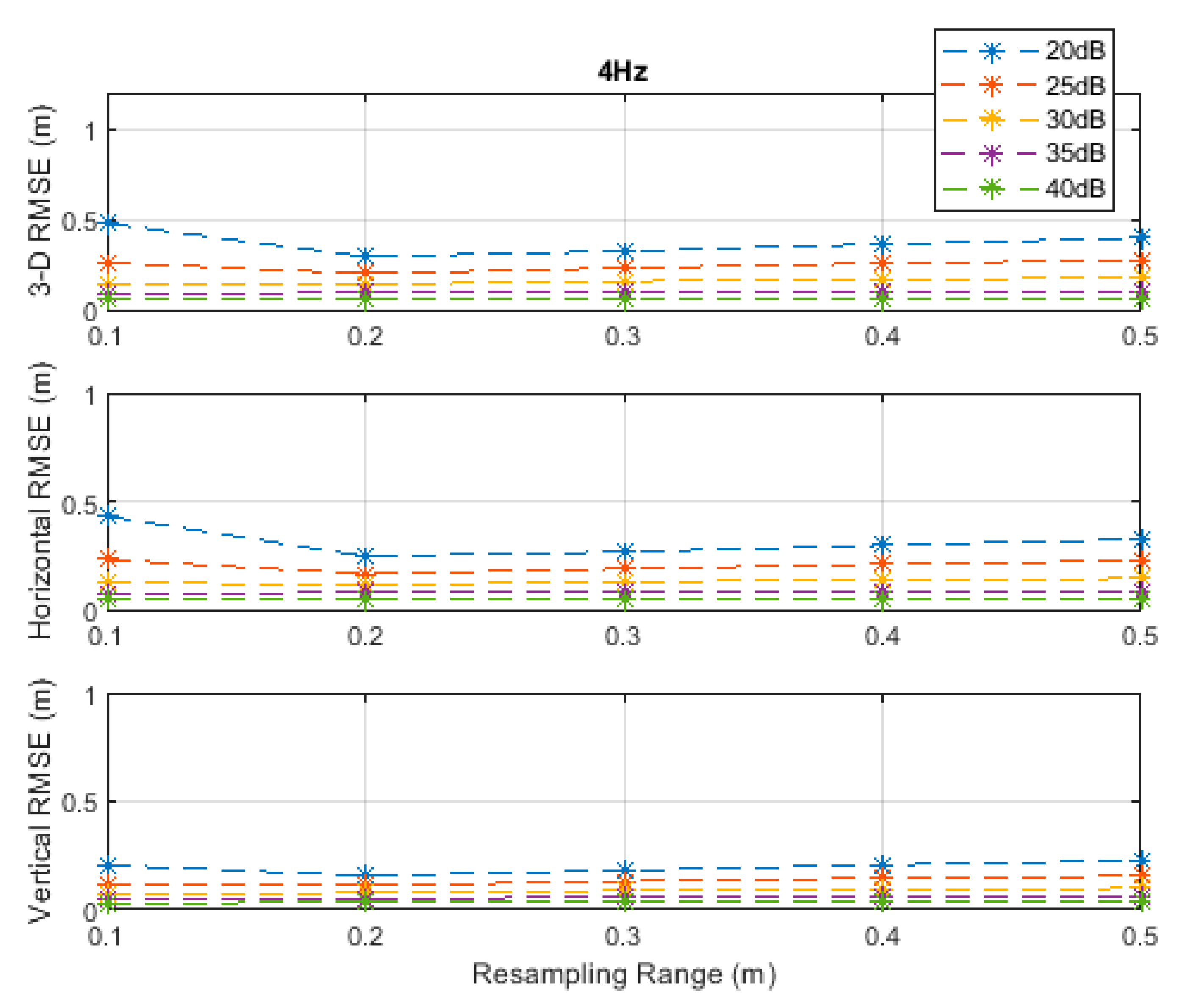
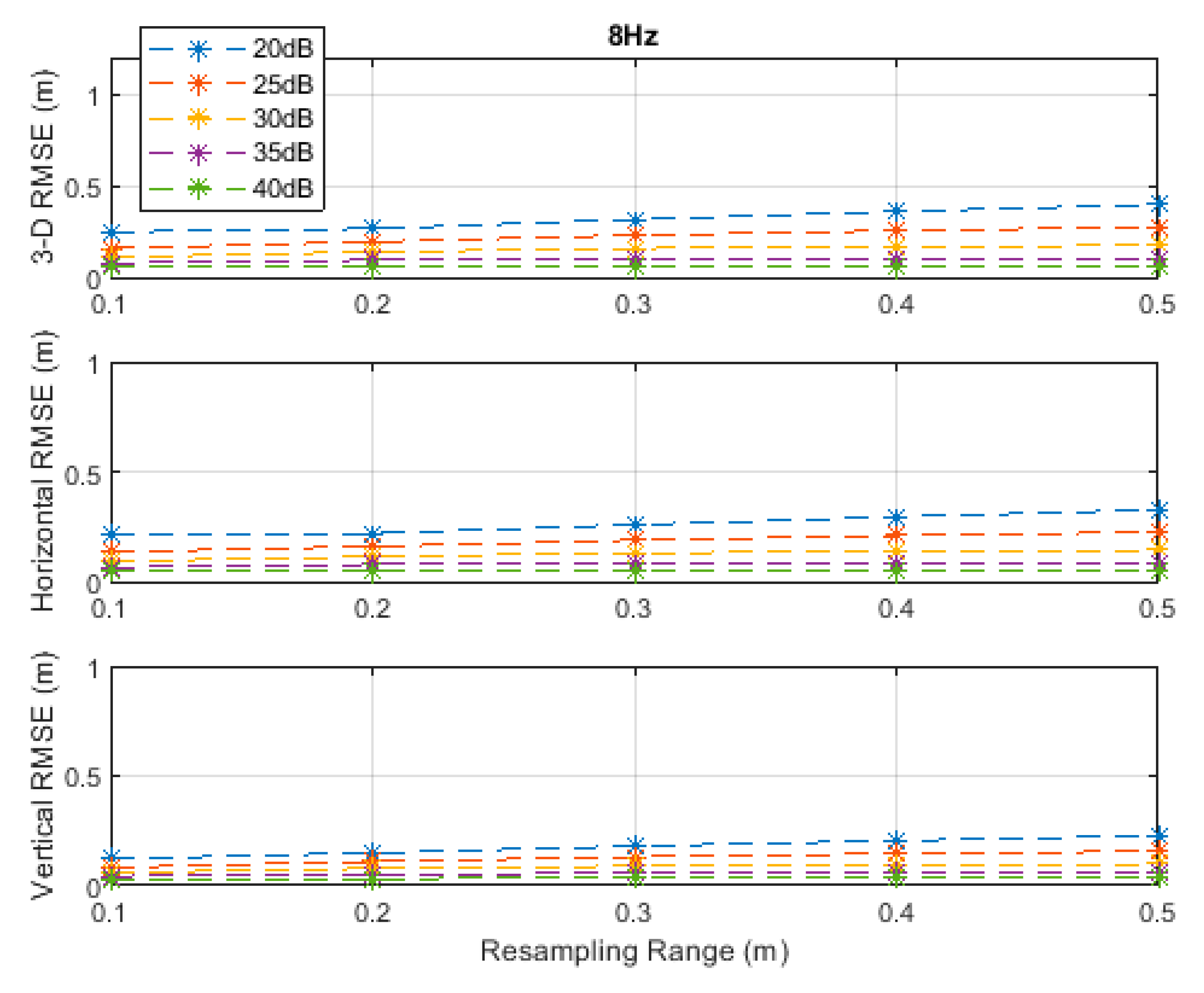
| RMSE (m) | 20 dB | 25 dB | 30 dB | 35 dB | 40 dB | Measurement Update Rate |
|---|---|---|---|---|---|---|
| 3D | 0.46 | 0.33 | 0.24 | 0.20 | 0.16 | |
| Horizontal | 0.37 | 0.27 | 0.20 | 0.16 | 0.13 | 1 Hz |
| Vertical | 0.26 | 0.19 | 0.14 | 0.12 | 0.09 | |
| 3D | 0.39 | 0.29 | 0.21 | 0.17 | 0.14 | |
| Horizontal | 0.32 | 0.24 | 0.17 | 0.14 | 0.11 | 2 Hz |
| Vertical | 0.23 | 0.16 | 0.12 | 0.10 | 0.08 | |
| 3D | 0.33 | 0.25 | 0.18 | 0.14 | 0.12 | |
| Horizontal | 0.27 | 0.20 | 0.15 | 0.12 | 0.10 | 4 Hz |
| Vertical | 0.19 | 0.15 | 0.10 | 0.08 | 0.07 | |
| 3D | 0.27 | 0.20 | 0.16 | 0.13 | 0.10 | |
| Horizontal | 0.22 | 0.17 | 0.13 | 0.10 | 0.08 | 8 Hz |
| Vertical | 0.16 | 0.11 | 0.09 | 0.07 | 0.06 | |
| 3D | 0.23 | 0.18 | 0.14 | 0.11 | 0.09 | |
| Horizontal | 0.19 | 0.14 | 0.12 | 0.09 | 0.07 | 16 Hz |
| Vertical | 0.13 | 0.10 | 0.08 | 0.06 | 0.05 |
| RMSE (m) | 20 dB | 25 dB | 30 dB | 35 dB | 40 dB | Measurement Update Rate |
|---|---|---|---|---|---|---|
| 3D | 0.48 | 0.34 | 0.26 | 0.20 | 0.16 | |
| Horizontal | 0.39 | 0.28 | 0.21 | 0.16 | 0.14 | 1 Hz |
| Vertical | 0.28 | 0.20 | 0.14 | 0.11 | 0.08 | |
| 3D | 0.41 | 0.31 | 0.23 | 0.18 | 0.13 | |
| Horizontal | 0.33 | 0.25 | 0.19 | 0.15 | 0.11 | 2 Hz |
| Vertical | 0.24 | 0.18 | 0.13 | 0.09 | 0.07 | |
| 3D | 0.36 | 0.26 | 0.19 | 0.15 | 0.11 | |
| Horizontal | 0.30 | 0.22 | 0.16 | 0.13 | 0.10 | 4 Hz |
| Vertical | 0.21 | 0.15 | 0.11 | 0.08 | 0.06 | |
| 3D | 0.30 | 0.22 | 0.17 | 0.14 | 0.10 | |
| Horizontal | 0.24 | 0.18 | 0.14 | 0.11 | 0.08 | 8 Hz |
| Vertical | 0.18 | 0.13 | 0.10 | 0.08 | 0.05 | |
| 3D | 0.26 | 0.19 | 0.14 | 0.12 | 0.09 | |
| Horizontal | 0.21 | 0.16 | 0.12 | 0.10 | 0.08 | 16 Hz |
| Vertical | 0.15 | 0.11 | 0.08 | 0.07 | 0.05 |
| RMSE (m) | 20 dB | 25 dB | 30 dB | 35 dB | 40 dB | Measurement Update Rate |
|---|---|---|---|---|---|---|
| 3D | 0.41 | 0.26 | 0.17 | 0.11 | 0.08 | |
| Horizontal | 0.34 | 0.22 | 0.13 | 0.09 | 0.06 | 1 Hz |
| Vertical | 0.23 | 0.15 | 0.10 | 0.06 | 0.04 | |
| 3D | 0.35 | 0.24 | 0.15 | 0.10 | 0.06 | |
| Horizontal | 0.30 | 0.19 | 0.12 | 0.08 | 0.05 | 2 Hz |
| Vertical | 0.19 | 0.13 | 0.08 | 0.05 | 0.03 | |
| 3D | 0.29 | 0.20 | 0.14 | 0.09 | 0.06 | |
| Horizontal | 0.25 | 0.16 | 0.11 | 0.07 | 0.05 | 4 Hz |
| Vertical | 0.16 | 0.11 | 0.07 | 0.05 | 0.03 | |
| 3D | 0.25 | 0.16 | 0.11 | 0.08 | 0.06 | |
| Horizontal | 0.22 | 0.13 | 0.09 | 0.06 | 0.05 | 8 Hz |
| Vertical | 0.12 | 0.08 | 0.06 | 0.04 | 0.03 | |
| 3D | 0.20 | 0.14 | 0.10 | 0.08 | 0.05 | |
| Horizontal | 0.17 | 0.12 | 0.09 | 0.06 | 0.04 | 16 Hz |
| Vertical | 0.11 | 0.08 | 0.06 | 0.04 | 0.03 |
| RMSE (m) | 20 dB | 25 dB | 30 dB | 35 dB | 40 dB | Measurement Update Rate |
|---|---|---|---|---|---|---|
| 3D | 0.52 | 0.34 | 0.24 | 0.17 | 0.13 | |
| Horizontal | 0.44 | 0.28 | 0.18 | 0.12 | 0.09 | 4 Hz |
| Vertical | 0.28 | 0.20 | 0.15 | 0.12 | 0.10 | |
| 3D | 0.45 | 0.30 | 0.20 | 0.15 | 0.11 | |
| Horizontal | 0.38 | 0.24 | 0.16 | 0.11 | 0.08 | 8 Hz |
| Vertical | 0.24 | 0.17 | 0.13 | 0.10 | 0.08 | |
| 3D | 0.36 | 0.25 | 0.18 | 0.13 | 0.10 | |
| Horizontal | 0.31 | 0.20 | 0.14 | 0.10 | 0.07 | 16 Hz |
| Vertical | 0.20 | 0.14 | 0.11 | 0.09 | 0.07 |
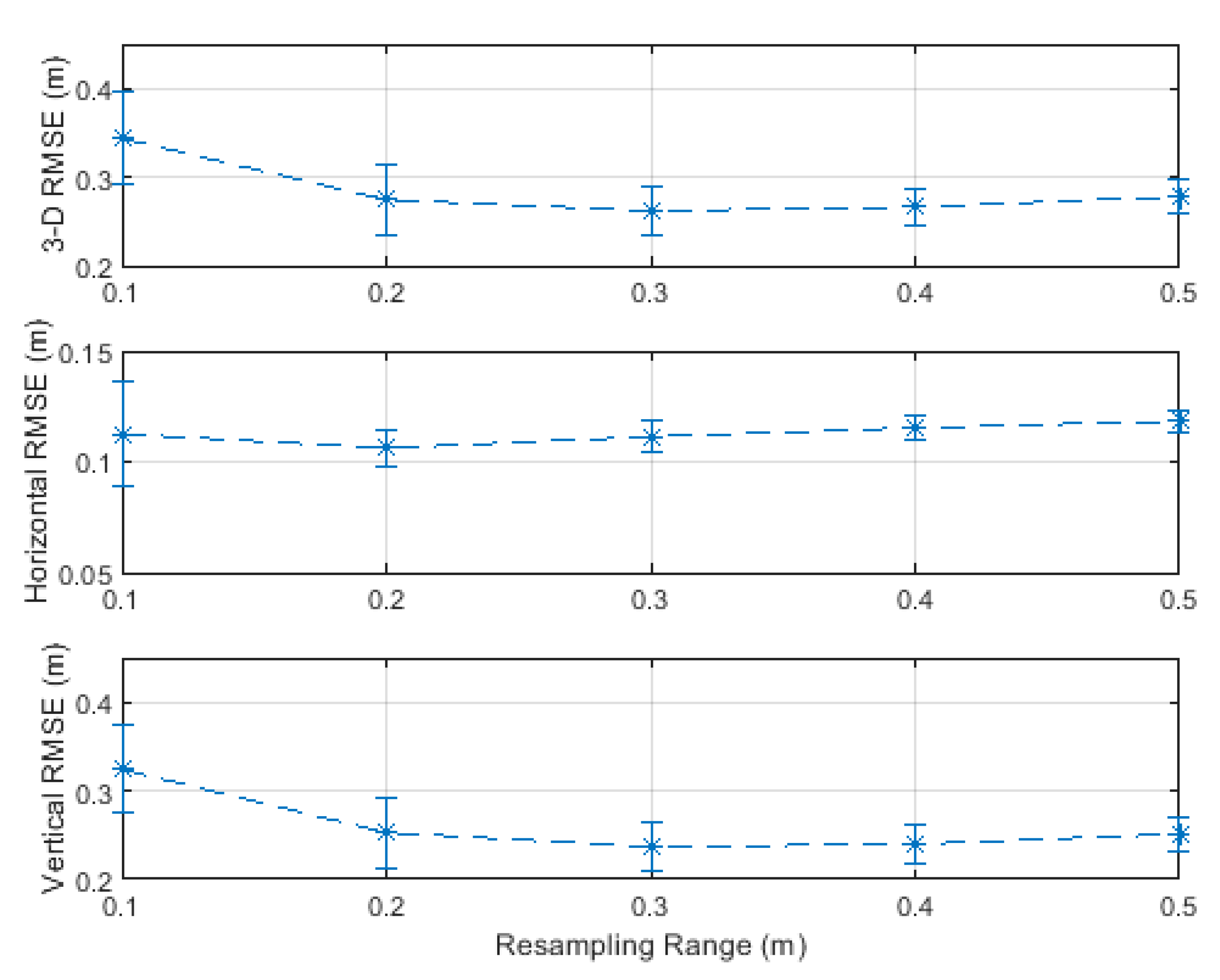
| RMSE (m) | Resampling Range (m) | ||||
|---|---|---|---|---|---|
| 0.1 | 0.2 | 0.3 | 0.4 | 0.5 | |
| 3D | 0.34 | 0.27 | 0.26 | 0.27 | 0.28 |
| 1-σ (cm) | 5.2 | 3.9 | 2.6 | 2.1 | 1.9 |
| Horizontal | 0.11 | 0.11 | 0.11 | 0.12 | 0.12 |
| 1-σ (cm) | 2.3 | 0.8 | 0.7 | 0.5 | 0.5 |
| Vertical | 0.32 | 0.25 | 0.24 | 0.24 | 0.25 |
| 1-σ (cm) | 4.9 | 4.0 | 2.7 | 2.1 | 1.9 |
© 2020 by the author. Licensee MDPI, Basel, Switzerland. This article is an open access article distributed under the terms and conditions of the Creative Commons Attribution (CC BY) license (http://creativecommons.org/licenses/by/4.0/).
Share and Cite
Khalaf-Allah, M. Particle Filtering for Three-Dimensional TDoA-Based Positioning Using Four Anchor Nodes. Sensors 2020, 20, 4516. https://doi.org/10.3390/s20164516
Khalaf-Allah M. Particle Filtering for Three-Dimensional TDoA-Based Positioning Using Four Anchor Nodes. Sensors. 2020; 20(16):4516. https://doi.org/10.3390/s20164516
Chicago/Turabian StyleKhalaf-Allah, Mohamed. 2020. "Particle Filtering for Three-Dimensional TDoA-Based Positioning Using Four Anchor Nodes" Sensors 20, no. 16: 4516. https://doi.org/10.3390/s20164516
APA StyleKhalaf-Allah, M. (2020). Particle Filtering for Three-Dimensional TDoA-Based Positioning Using Four Anchor Nodes. Sensors, 20(16), 4516. https://doi.org/10.3390/s20164516