Data Augmentation for Motor Imagery Signal Classification Based on a Hybrid Neural Network

 ,
,
Abstract
1. Introduction
2. Method
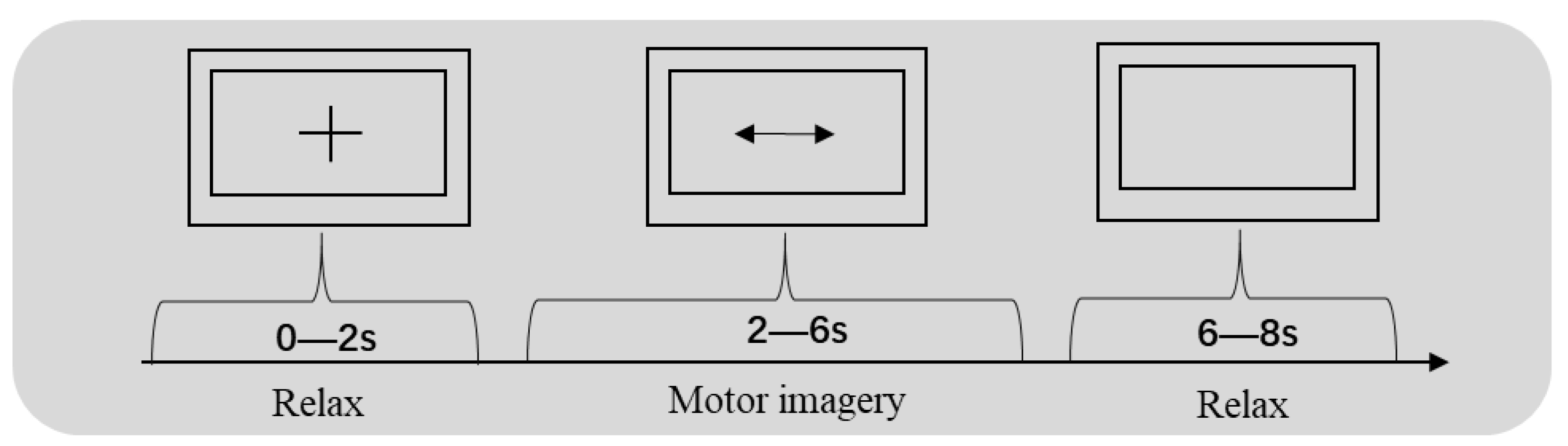
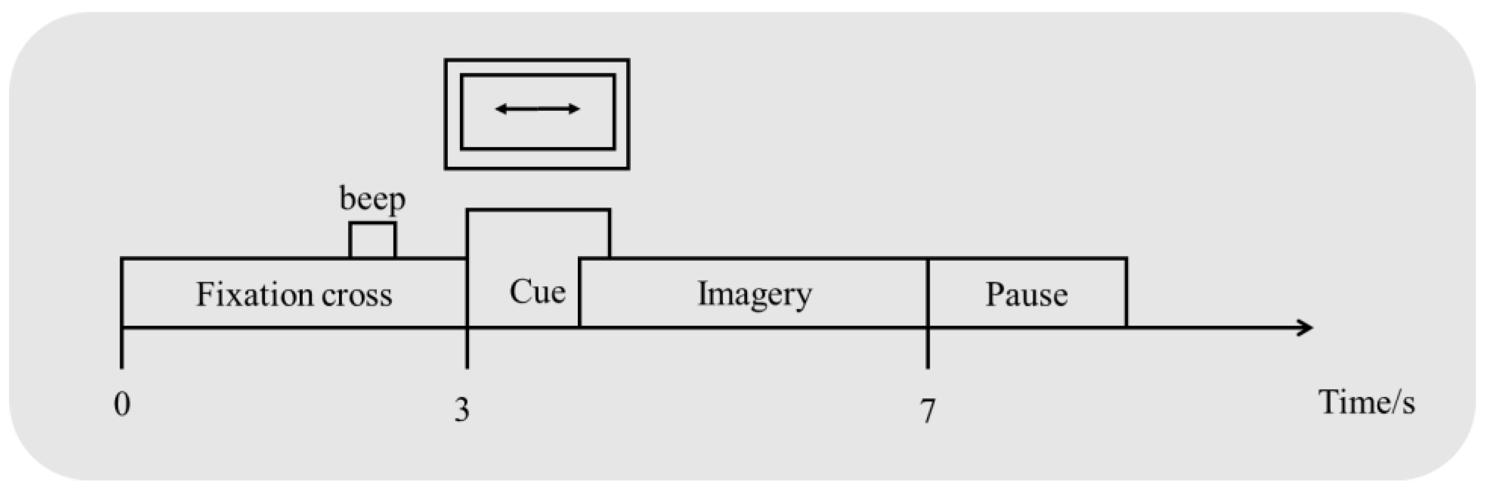
2.1. Datasets
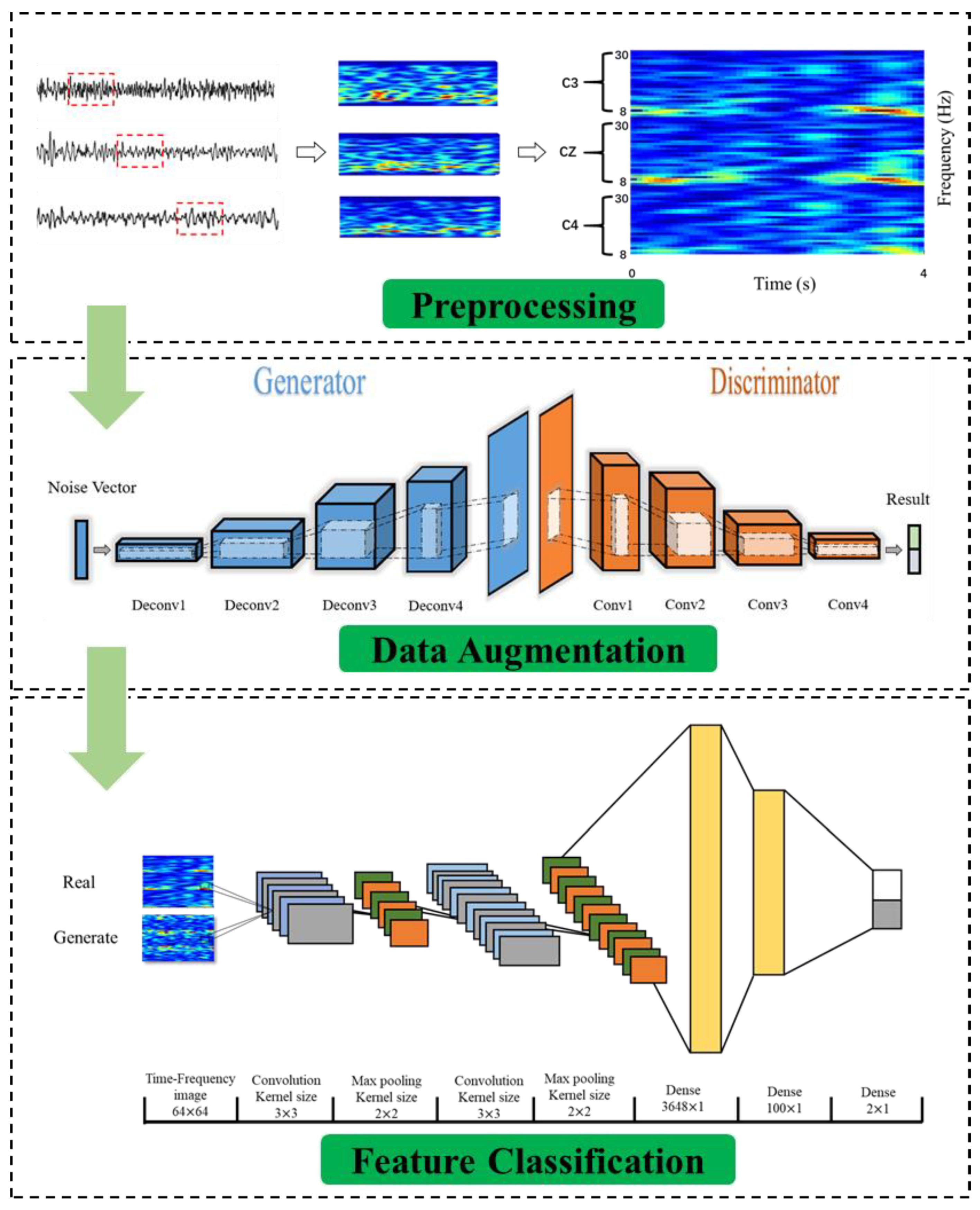
2.2. Preprocessing of the Raw Data
2.3. Different Data Augmentation Models
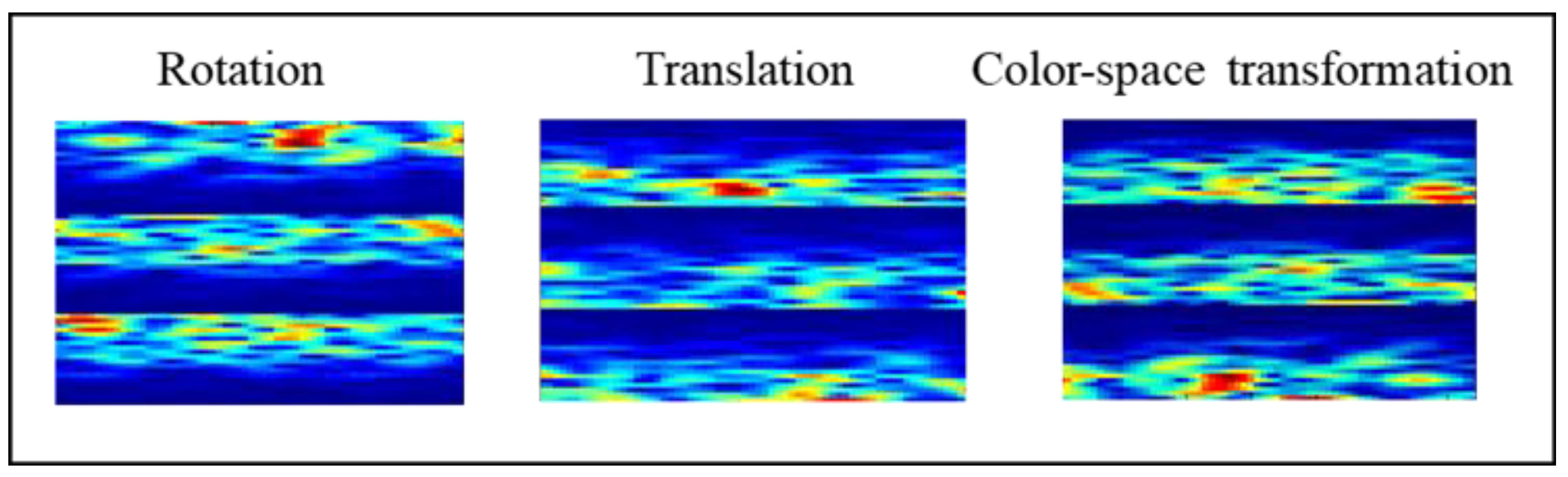
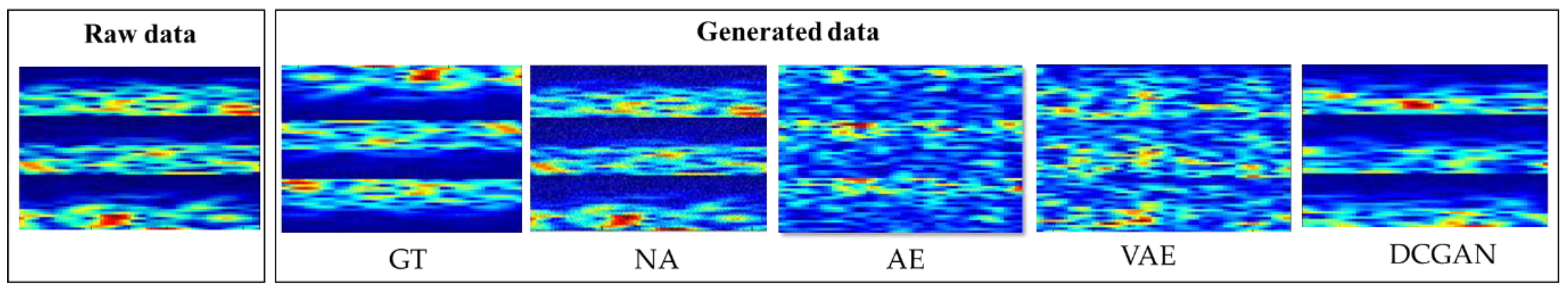
2.3.1. Geometric Transformation (GT)
- (1)
- Rotate the image 180° right or left on the x-axis (rotation);
- (2)
- Shift the images left, right, up, or down; the remaining space is filled with random noise (translation);
- (3)
- Perform augmentations in the color space (color-space transformation).
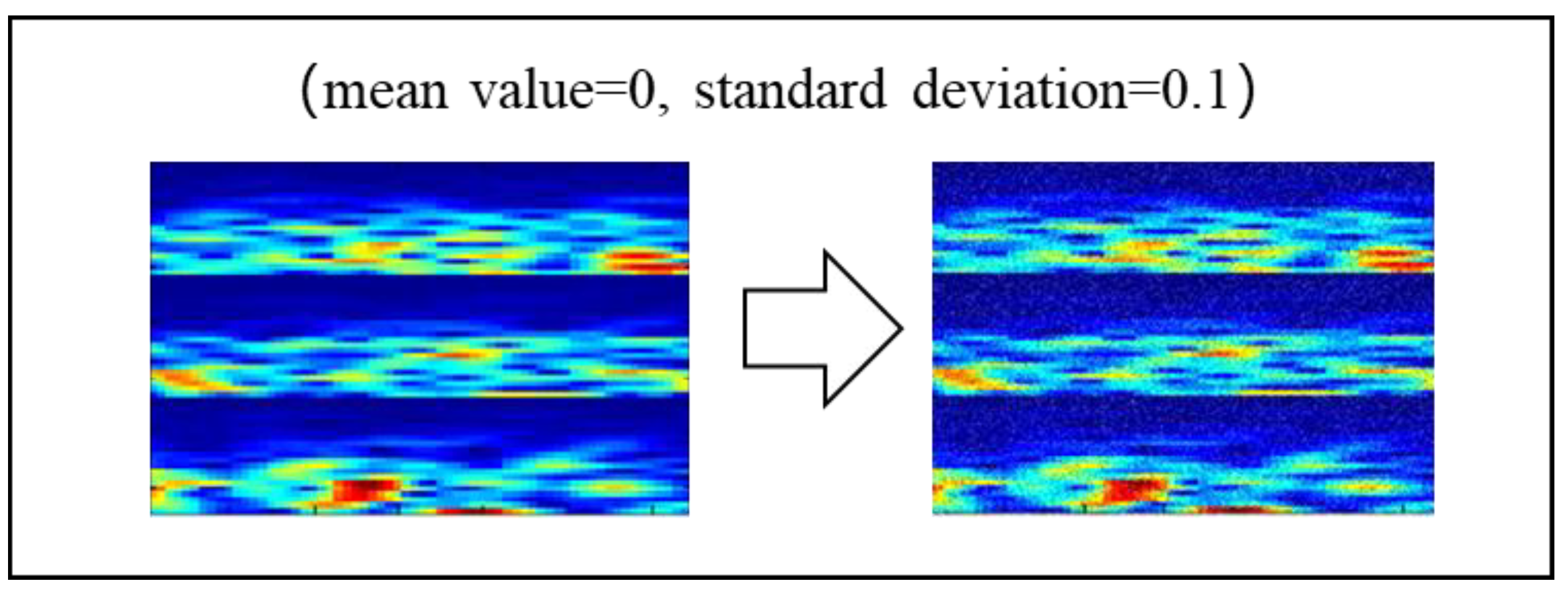
2.3.2. Noise Addition (NA)
2.3.3. Generative Model
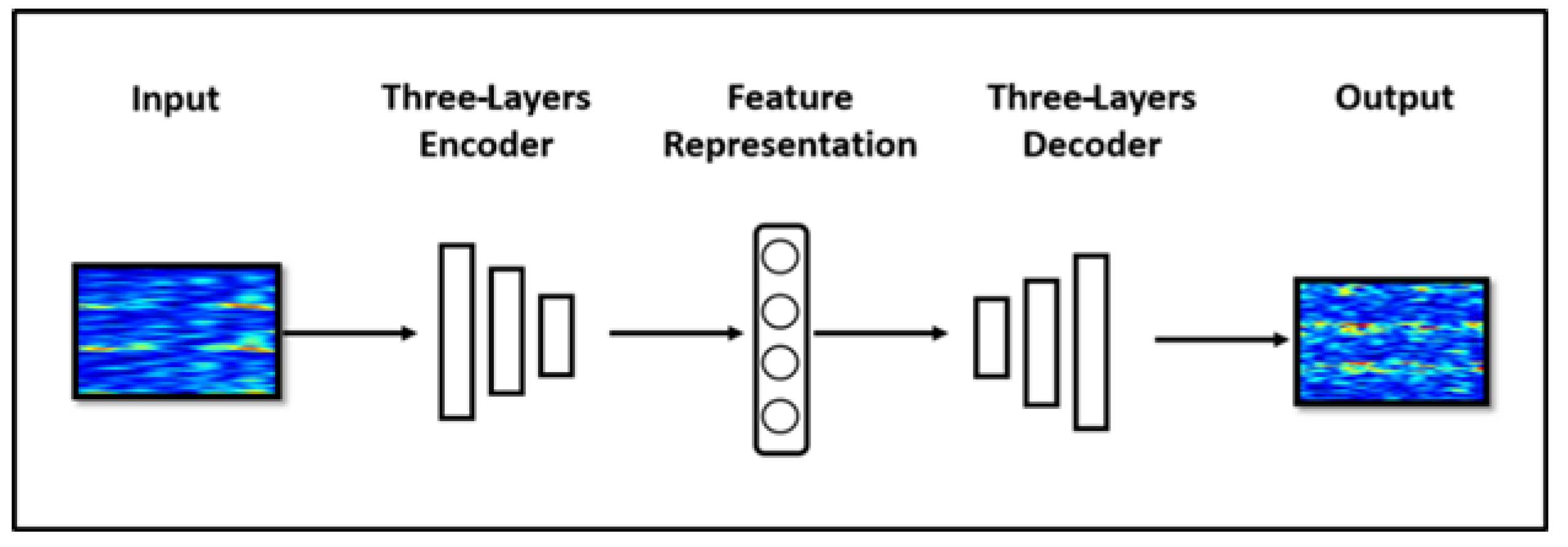
a. Autoencoder (AE)
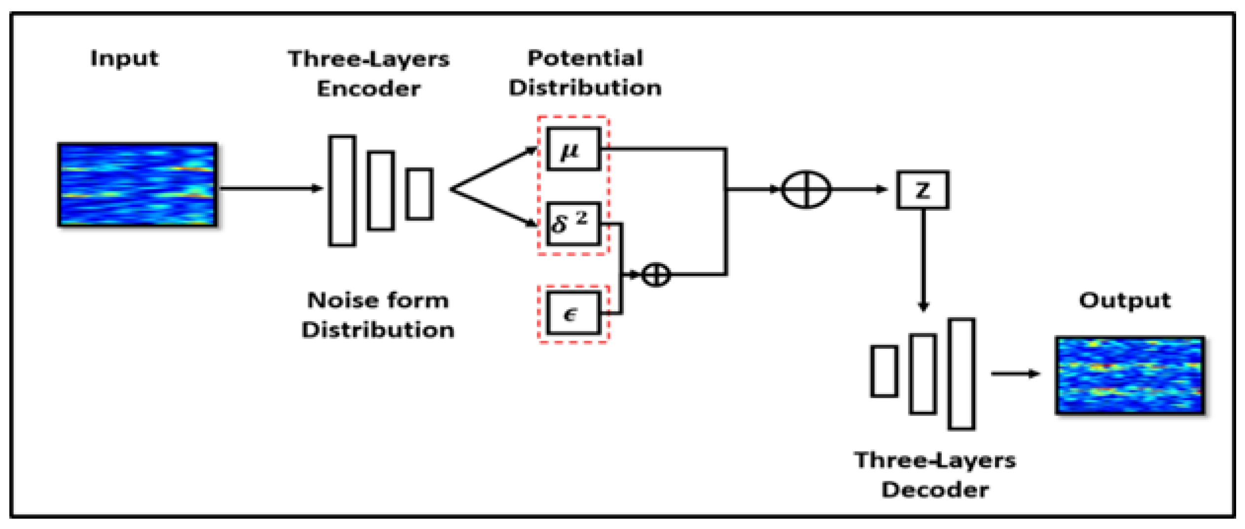
b. Variational Autoencoder (VAE)
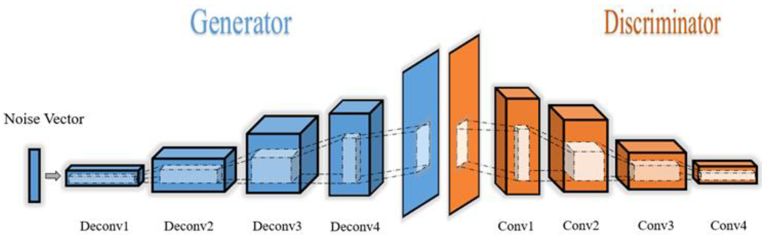
c. Deep Convolutional Generative Adversarial Networks (DCGANs)
- The pooling layer is replaced by fractional-strided convolutions in the generator and by strided convolutions in the discriminator.
- Batch normalization is used in the generator and discriminator, and there is no fully connected layer.
- In the generator, all layers except for the output use the rectified linear unit (ReLU) as an activation function; the output layer use tanh.
- All layers use the leaky ReLU as the action function in the discriminator.
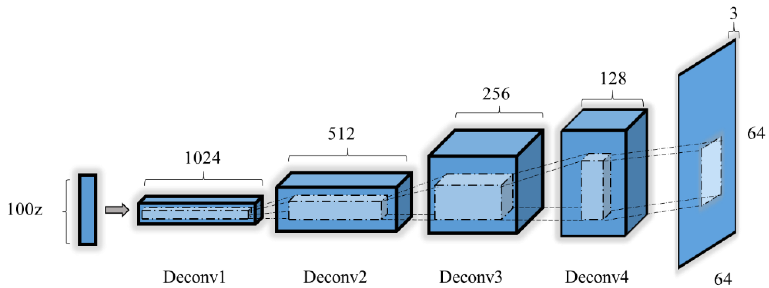
2.3.4. Generator Model
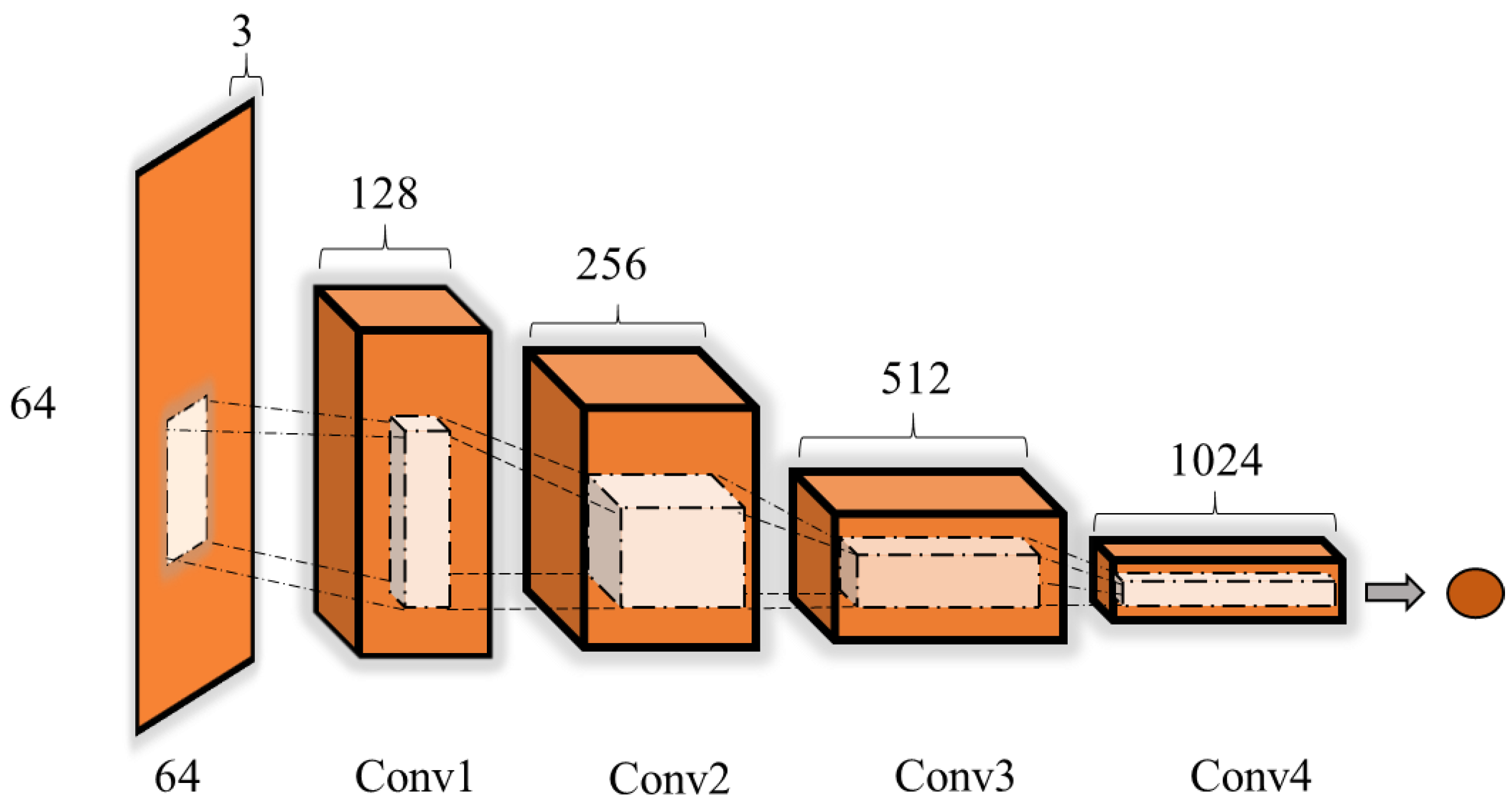
2.3.5. Discriminator Model
2.4. Performance Verification of the Data Augmentation
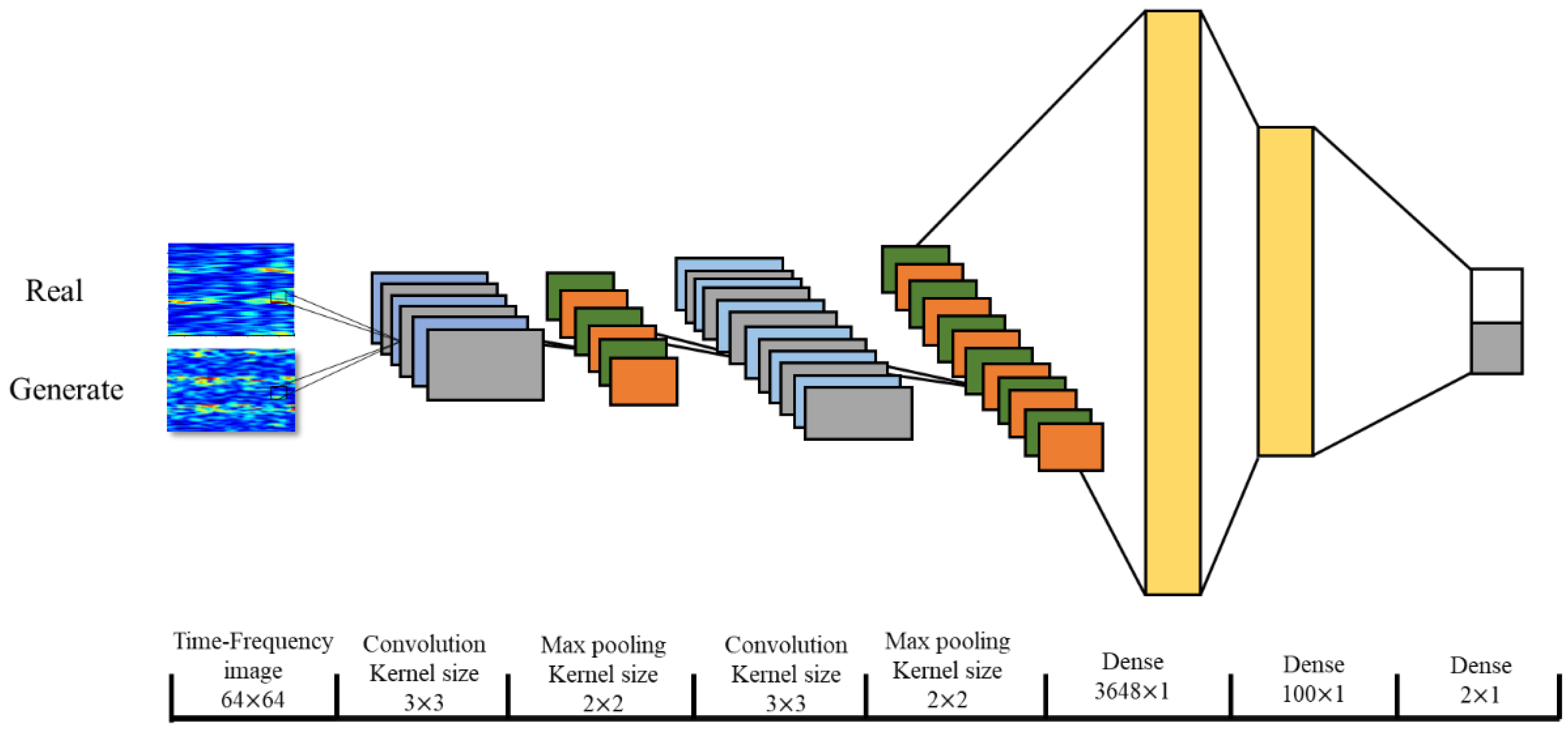
2.5. Evaluation of the MI Classification Performance after the Augmentation
3. Experimental Results
3.1. Results of the Freéchet Inception Distances for Different Data Augmentation Methods
- One subject for each of 200 trials and 720 trials in datasets 1 and 2b, respectively. A larger-scale training data improved the robustness and generalization of the model.
- Due to the difference in sampling rate, the sample sizes of the two datasets were 400 and 1000 (datasets 1 and 2b, respectively). More samples would be helpful to improve the resolution of the spectrogram.
- During the experimental process, dataset 2b designed the cue-based screening paradigm that aimed to enhance the attention of the subjects before imagery. However, there was no similar set in dataset 1. This setting may lead to a more consistent feature distribution and higher quality for MI spectrogram data.
3.2. Classification Performance of Different Data Augmentation Methods
3.3. Comparison with Existing Classification Methods
4. Discussion
5. Conclusions
Author Contributions
Funding
Acknowledgments
Conflicts of Interest
References
- Yuan, H.; He, B. Brain-computer interfaces using sensorimotor rhythms: Current state and future perspectives. IEEE Trans. Biomed. Eng. 2014, 61, 1425–1435. [Google Scholar] [CrossRef] [PubMed]
- Nicolas-Alonso, L.F.; Gomez-Gil, J. Brain computer interfaces, a review. Sensors 2012, 12, 1211–1279. [Google Scholar] [CrossRef] [PubMed]
- Bonassi, G.; Biggio, M.; Bisio, A.; Ruggeri, P.; Bove, M.; Acanzino, L. Provision of somatosensory inputs during motor imagery enhances learning-induced plasticity in human motor cortex. Sci. Rep. 2017, 7, 1–10. [Google Scholar]
- Munzert, J.; Lorey, B.; Zentgraf, K. Cognitive motor processes: The role of motor imagery in the study of motor representations. Brain Res. Rev. 2009, 60, 306–326. [Google Scholar] [CrossRef] [PubMed]
- Coyle, D.; Stow, J.; Mccreadie, K.; Mcelligott, J.; Carroll, A. Sensorimotor Modulation Assessment and Brain-Computer Interface Training in Disorders of Consciousness. Arch. Phys. Med. Rehabil. 2015, 96, S62–S70. [Google Scholar] [CrossRef]
- Anderson, W.S.; Lenz, F.A. Review of motor and phantom-related imagery. Neuroreport 2011, 22, 939–942. [Google Scholar] [CrossRef]
- Phothisonothai, M.; Nakagawa, M. EEG-based classification of motor imagery tasks using fractal dimension and neural network for brain-computer interface. IEICE Trans. Inf. Syst. 2008, 91, 44–53. [Google Scholar] [CrossRef]
- Schlögl, A.; Vidaurre, C.; Müller, K.R. (Eds.) Adaptive methods in BCI research-an introductory tutorial. In Brain-Computer Interfaces Revolutionizing Human-Computer Interfaces; Springer: Berlin/Heidelberg, Germany, 2010; pp. 331–355. [Google Scholar]
- Song, X.; Yoon, S.C.; Perera, V. Adaptive Common Spatial Pattern for Single-Trial EEG Classifcation in Multisubject BCI. In Proceedings of the International IEEE/EMBS Conference on Neural Engineering, San Diego, CA, USA, 6–8 November 2013; pp. 411–414. [Google Scholar]
- Vidaurre, C.; Schlögl, A.; Cabeza, R.; Scherer, R.; Pfurtscheller, G. Study of on-line adaptive discriminant analysis for EEG-based brain computer interface. IEEE Trans. Biomed. Eng. 2007, 54, 550–556. [Google Scholar] [CrossRef]
- Woehrle, H.; Krell, M.M.; Straube, S.; Kim, S.K.; Kirchner, E.A.; Kirchner, F. An adaptive spatial flter for user-independent single trial detection of event-related potentials. IEEE Trans. Biomed. Eng. 2015, 62, 1696–1705. [Google Scholar] [CrossRef]
- Duan, X.; Xie, S.; Xie, X.; Meng, Y.; Xu, Z. Quadcopter Flight Control Using a Non-invasive Multi-Modal Brain Computer Interface. Frontiers. Neurorobotics 2019, 13, 23. [Google Scholar] [CrossRef]
- Song, X.; Shibasaki, R.; Yuan, N.J.; Xie, X.; Li, T.; Adachi, R. DeepMob: Learning deep knowledge of human emergency behavior and mobility from big and heterogeneous data. ACM Trans. Inf. Syst. (TOIS) 2017, 35, 1–19. [Google Scholar] [CrossRef]
- Alom, M.Z.; Taha, T.M.; Yakopcic, C.; Westberg, S.; Sidike, P.; Nasrin, M.S.; Van Esesn, B.C.; Awwal, A.A.S.; Asari, V.K. The history began from alexnet: A comprehensive survey on deep learning approaches. arXiv 2018, arXiv:1803.01164. [Google Scholar]
- Zhong, Z.; Jin, L.; Xie, Z. High performance offline handwritten chinese character recognition using googlenet and directional feature maps. In Proceedings of the 2015 13th International Conference on Document Analysis and Recognition (ICDAR), Tunis, Tunisia, 23–26 August 2015; pp. 846–850. [Google Scholar]
- Cooney, C.; Folli, R.; Coyle, D. Optimizing Layers Improves CNN Generalization and Transfer Learning for Imagined Speech Decoding from EEG. In Proceedings of the 2019 IEEE International Conference on Systems, Man and Cybernetics (SMC), Bari, Italy, 6–9 October 2019; pp. 1311–1316. [Google Scholar]
- LeCun, Y.; Bengio, Y.; Hinton, G. Deep learning. Nature 2015, 521, 436. [Google Scholar] [CrossRef]
- Salamon, J.; Bello, J.P. Deep convolutional neural networks and data augmentation for environmental sound classification. IEEE Signal. Process. Lett. 2017, 24, 279–283. [Google Scholar] [CrossRef]
- Roy, Y.; Banville, H.; Albuquerque, I.; Gramfort, A.; Falk, T.H.; Faubert, J. Deep learning-based electroencephalography analysis: A systematic review. J. Neural Eng. 2019, 16, 051001. [Google Scholar] [CrossRef]
- Perez-Benitez, J.L.; Perez-Benitez, J.A.; Espina Hernandez, J.H. Development of a brain computer interface interface using multi-frequency visual stimulation and deep neural networks. In Proceedings of the International Conference on Electronics, Communications and Computers, Cholula, Mexico, 21–23 February 2018; pp. 18–24. [Google Scholar]
- Setio, A.A.A.; Ciompi, F.; Litjens, G.; Gerke, P.; Jacobs, C.; Van Riel, S.J.; Wille, M.M.W.; Naqibullah, M.; Sanchez, C.I.; Van Ginneken, B. Pulmonary Nodule Detection in CT Images: False Positive Reduction Using Multi-View Convolutional Networks. IEEE Trans. Med. Imaging 2016, 35, 1160–1169. [Google Scholar] [CrossRef]
- Pereira, S.; Pinto, A.; Alves, V.; Silva, C.A. Brain tumor segmentation using convolutional neural networks in MRI images. IEEE Trans. Med. Imaging 2016, 35, 1240–1251. [Google Scholar] [CrossRef]
- Shao, S.; Wang, P.; Yan, R. Generative adversarial networks for data augmentation in machine fault diagnosis. Comput. Ind. 2019, 106, 85–93. [Google Scholar] [CrossRef]
- Frid-Adar, M.; Diamant, I.; Klang, E.; Amitai, M.; Goldberger, J.; Greenspan, H. GAN-based synthetic medical image augmentation for increased CNN performance in liver lesion classification. Neurocomputing 2018, 321, 321–331. [Google Scholar] [CrossRef]
- Abdelfattah, S.M.; Abdelrahman, G.M.; Wang, M. Augmenting the size of EEG datasets using generative adversarial networks. In Proceedings of the 2018 IEEE International Joint Conference on Neural Networks (IJCNN), Rio, Brazil, 8–13 July 2018; pp. 1–6. [Google Scholar]
- Dai, G.; Zhou, J.; Huang, J.; Wang, N. HS-CNN: A CNN with hybrid convolution scale for EEG motor imagery classification. J. Neural Eng. 2020, 17, 016025. [Google Scholar] [CrossRef] [PubMed]
- Li, Y.; Zhang, X.R.; Zhang, B.; Lei, M.Y.; Cui, W.G.; Guo, Y.Z. A Channel-Projection Mixed-Scale Convolutional Neural Network for Motor Imagery EEG Decoding. IEEE Trans. Neural Syst. Rehabil. Eng. 2019, 27, 1170–1180. [Google Scholar] [CrossRef] [PubMed]
- Zhang, Z.; Duan, F.; Solé-Casals, J.; Dinares-Ferran, J.; Cichocki, A.; Yang, Z.; Sun, Z. A novel deep learning approach with data augmsentation to classify motor imagery signals. IEEE Access 2019, 7, 15945. [Google Scholar] [CrossRef]
- Ko, W.; Jeon, E.; Lee, J.; Suk, H.I. Semi-Supervised Deep Adversarial Learning for Brain-Computer Interface. In Proceedings of the 2019 7th International Winter Conference on Brain-Computer Interface (BCI), Gangwon, Korea, 18–20 February 2019; pp. 1–4. [Google Scholar]
- Freer, D.; Yang, G.Z. Data augmentation for self-paced motor imagery classification with C-LSTM. J. Neural Eng. 2019, 17, 016041. [Google Scholar] [CrossRef] [PubMed]
- Majidov, I.; Whangbo, T. Efficient Classification of Motor Imagery Electroencephalography Signals Using Deep Learning Methods. Sensors 2019, 19, 1736. [Google Scholar] [CrossRef] [PubMed]
- Shovon, T.H.; Al Nazi, Z.; Dash, S.; Hossain, F. Classification of Motor Imagery EEG Signals with multi-input Convolutional Neural Network by augmenting STFT. In Proceedings of the 2019 5th International Conference on Advances in Electrical Engineering (ICAEE), Dhaka, Bangladesh, 26–28 September 2019; pp. 398–403. [Google Scholar]
- Lotte, F. Generating Artificial EEG Signals To Reduce BCI Calibration Time. In Proceedings of the 5th International Brain-Computer Interface Workshop, Graz, Austria, 22–24 September 2011; pp. 176–179. [Google Scholar]
- Shorten, C.; Khoshgoftaar, T.M. A survey on Image Data Augmentation for Deep Learning. J. Big Data 2019, 6, 1–48. [Google Scholar] [CrossRef]
- Logan, E.; Brandon, T.; Dimitris, T.; Ludwig, S.; Aleksander, M. A rotation and a translation sufce: Fooling CNNs with simple transformations. arXiv 2018, arXiv:1712.02779. [Google Scholar]
- Goodfellow I., J.; Shlens, J.; Szegedy, C. Explaining and harnessing adversarial examples. arXiv 2015, arXiv:1412.6572. [Google Scholar]
- Wang, F.; Zhong, S.; Peng, J.; Jiang, J.; Liu, Y. Data augmentation for eeg-based emotion recognition with deep convolutional neural networks. In Proceedings of the International Conference on Multimedia Modeling, 5–7 February 2018; Springer: Cham, Bangkok, Thailand; pp. 82–93. [Google Scholar]
- He, K.; Zhang, X.; Ren, S.; Sun, J. Deep Residual Learning for Image Recognition. In Proceedings of the 2016 IEEE Conference on Computer Vision and Pattern Recognition (CVPR), Las Vegas, NV, USA, 27–30 June 2016; pp. 770–778. [Google Scholar]
- Terrance, V.; Graham, W.T. Dataset augmentation in feature space. In Proceedings of the International Conference on Machine Learning (ICML), Sydney, Australia, 10–11 August 2017. [Google Scholar]
- Gao, Y.; Kong, B.; Mosalam, K.M. Deep leaf-bootstrapping generative adversarial network for structural image data augmentation. Comput. Civ. Infrastruct. Eng. 2019, 34, 755–773. [Google Scholar] [CrossRef]
- Hartmann, K.G.; Schirrmeister, R.T.; Ball, T. EEG-GAN: Generative adversarial networks for electroencephalograhic (EEG) brain signals. arXiv 2018, arXiv:1806.01875. [Google Scholar]
- BCI Competition 2008—Graz Data Sets 2A and 2B. Available online: http://www.bbci.de/competition/iv/ (accessed on 30 May 2019).
- Pfurtscheller, G.; Da Silva, F.L. Event-related EEG/MEG synchronization and desynchronization: Basic principles. Clin. Neurophysiol. 1999, 110, 1842–1857. [Google Scholar] [CrossRef]
- Griffin, D.; Lim, J. Signal estimation from modified short-time Fourier transform. IEEE Trans. Acoust. SpeechSignal Process. 1984, 32, 236–243. [Google Scholar] [CrossRef]
- Kıymık, M.; Güler, I.; Dizibüyük, A.; Akın, M. Comparison of STFT and wavelet transform methods in determining epileptic seizure activity in EEG signals for real-time application. Comput. Boil. Med. 2005, 35, 603–616. [Google Scholar] [CrossRef] [PubMed]
- Pfurtscheller, G.; Neuper, C. Motor imagery and direct brain-computer communication. Proc. IEEE 2001, 89, 1123–1134. [Google Scholar] [CrossRef]
- Lemley, J.; Barzrafkan, S.; Corcoran, P. Smart augmentation learning an optimal data augmentation strategy. IEEE Access 2017, 5, 5858–5869. [Google Scholar] [CrossRef]
- Cubuk, E.D.; Zoph, B.; Mane, D.; Vasudevan, V.; Le, Q.V. AutoAugment: Learning Augmentation Policies from Data. arXiv 2018, arXiv:1805.09501. [Google Scholar]
- Moreno-Barea, J.; Strazzera, F.; JerezUrda, D.; Franco, L. Forward Noise Adjustment Scheme for Data Augmentation. In Proceedings of the IEEE Symposium Series on Computational Intelligence (IEEE SSCI 2018), Bengaluru, India, 18–26 November 2018; pp. 728–734. [Google Scholar]
- Kingma, D.P.; Welling, M. Auto-encoding variational bayes. arXiv 2013, arXiv:1312.6114. [Google Scholar]
- Github. 2019. Available online: https://github.com/5663015/galaxy_generation (accessed on 2 August 2019).
- Goodfellow, I.; Pouget-Abadie, J.; Mirza, M.; Xu, B.; Warde-Farely, D.; Ozair, S.; Courville, A.; Bengio, Y. Generative Adversarial Nets. In Proceedings of the International Conference on Neural Information Processing Systems, Montreal, QC, Canada, 8–12 December 2014; pp. 2672–2680. [Google Scholar]
- Salimans, T.; Goodfellow, I.; Zaremba, W.; Cheung, V.; Radford, A.; Chen, X. (Eds.) Improved Techniques for Training GANs. In Advances in Neural Information Processing Systems; NIPS: Barcelona, Spain, 2016; pp. 2234–2242. [Google Scholar]
- Radford, A.; Metz, L.; Chintala, S. Unsupervised representation learning with deep convolutional generative adversarial networks. arXiv 2015, arXiv:1511.06434. [Google Scholar]
- Dosovitskiy, A.; Fischer, P.; Springenberg, J.T.; Riedmiller, M.; Brox, T. Discriminative Unsupervised Feature Learning with Exemplar Convolutional Neural Networks. IEEE Trans. Pattern Anal. Mach. Intell. 2015, 38, 1734–1747. [Google Scholar] [CrossRef]
- Xu, Q.; Huang, G.; Yuan, Y.; Guo, C.; Sun, Y.; Wu, F.; Weinberger, K.Q. An empirical study on evaluation metrics of generative adversarial networks. arXiv 2018, arXiv:1806.07755. [Google Scholar]
- Szegedy, C.; Liu, W.; Jia, Y.; Sermanet, P.; Reed, S.; Anguelov, D.; Erhan, D.; Vanhoucke, V.; Rabinovich, A. Going deeper with convolutions. In Proceedings of the 2015 IEEE Conference on Computer Vision and Pattern Recognition (CVPR), Boston, MA, USA, 7–12 June 2015; pp. 1–9. [Google Scholar]
- Tabar, Y.R.; Halici, U. A novel deep learning approach for classification of EEG motor imagery signals. J. Neural Eng. 2016, 14, 16003. [Google Scholar] [CrossRef]
- Schirrmeister, R.T.; Springenberg, J.T.; Fiederer, L.; Glasstetter, M.; Eggensperger, K.; Tangermann, M.; Hutter, F.; Burgard, W.; Ball, T. Deep learning with convolutional neural networks for EEG decoding and visualization. Hum. Brain Mapp. 2017, 38, 5391–5420. [Google Scholar] [CrossRef] [PubMed]
- Craik, A.; He, Y.; Contreras-Vidal, J.L. Deep learning for electroencephalogram (EEG) classification tasks: A review. J. Neural Eng. 2019, 16, 031001. [Google Scholar] [CrossRef] [PubMed]
- Rodríguez, J.D.; Pérez, A.; Lozano, J.A. Sensitivity Analysis of k-Fold Cross Validation in Prediction Error Estimation. IEEE Trans. Pattern Anal. Mach. Intell. 2009, 32, 569–575. [Google Scholar] [CrossRef] [PubMed]
- Ang, K.K.; Chin, Z.Y.; Wang, C.; Guan, C.; Zhang, H. Filter Bank Common Spatial Pattern Algorithm on BCI Competition IV Datasets 2a and 2b. Front. Behav. Neurosci. 2012, 6, 39. [Google Scholar] [CrossRef]
- Rong, Y.; Wu, X.; Zhang, Y. Classification of motor imagery electroencephalography signals using continuous small convolutional neural network. Int. J. Imaging Syst. Technol. 2020. [Google Scholar] [CrossRef]
- Dai, M.; Zheng, D.; Na, R.; Wang, S.; Zhang, S. EEG Classification of Motor Imagery Using a Novel Deep Learning Framework. Sensors 2019, 19, 551. [Google Scholar] [CrossRef]
- Malan, N.S.; Sharma, S. Feature selection using regularized neighbourhood component analysis to enhance the classification performance of motor imagery signals. Comput. Boil. Med. 2019, 107, 118–126. [Google Scholar] [CrossRef]
- Bustios, P.; Rosa, J.L. Restricted exhaustive search for frequency band selection in motor imagery classification. In Proceedings of the 2017 International Joint Conference on Neural Networks (IJCNN), Anchorage, AK, USA, 14–19 May 2017; IEEE: Anchorage, AK, USA; pp. 4208–4213. [Google Scholar]
- Saa, J.F.D.; Cetin, M. Hidden conditional random fields for classification of imaginary motor tasks from eeg data. In Proceedings of the 2011 19th IEEE European Signal Processing Conference, Barcelona, Spain, 29 August–2 September 2011; pp. 171–175. [Google Scholar]
- Vernon, L.; Amelia, S.; Nicholas, W.; Gordon, S.M.; Hung, C.P.; Lance, B.J. EEGNet: A compact convolutional neural network for EEG-based brain—Computer interfaces. J. Neural Eng. 2018, 15, 056013. [Google Scholar]
- Chaudhary, S.; Taran, S.; Bajaj, V.; Sengur, A. Convolutional Neural Network Based Approach Towards Motor Imagery Tasks EEG Signals Classification. IEEE Sens. J. 2019, 19, 4494–4500. [Google Scholar] [CrossRef]
- Ponce, C.R.; Xiao, W.; Schade, P.; Hartmann, T.S.; Kreiman, G.; Livingstone, M.S. Evolving Images for Visual Neurons Using a Deep Generative Network Reveals Coding Principles and Neuronal Preferences. Cell 2019, 177, 999–1009.e10. [Google Scholar] [CrossRef]
- Padfield, N.; Zabalza, J.; Zhao, H.; Masero, V.; Ren, J. EEG-Based Brain-Computer Interfaces Using Motor-Imagery: Techniques and Challenges. Sensors 2019, 19, 1423. [Google Scholar] [CrossRef] [PubMed]
- Rodríguez-Ugarte, M.; Iáñez, E.; Ortiz, M.; Azorín, J.M. Effects of tDCS on Real-Time BCI Detection of Pedaling Motor Imagery. Sensors 2018, 18, 1136. [Google Scholar] [CrossRef] [PubMed]
- Zanini, R.A.; Colombini, E.L. Parkinson’s Disease EMG Data Augmentation and Simulation with DCGANs and Style Transfer. Sensors 2020, 30, 2605. [Google Scholar] [CrossRef] [PubMed]


| Electroencephalogram (EEG) Pattern | Augmentation Methods | Limitations |
|---|---|---|
| Motor movement/imagery [25] | Recurrent generative adversarial network (GAN) | Shows good potential for time-series data generation but has limitations for image generation |
| Motor imagery [26] | Segmentation–recombination | Limited improvement for the diversity of feature distribution |
| Motor imagery [27] | Noise addition | May change and adversely affect the feature distribution |
| Motor imagery [28] | Empirical mode decomposition | Suitable for time-series data generation but has limitations for image generation; |
| Motor imagery [29] | GAN | instability during training may result in meaningless output |
| Motor imagery [30] | Geometric transformation and noise addition | Easy to obtain motion-related information after geometric transformation but limited improvement for the diversity of data generation |
| Motor imagery [31] | Sliding windows | Easy to lose motion-related information after changing the window size |
| Motor imagery [32] | Geometric transformation | Easy to lose motion-related information after the geometric transformation |
| Layers | Type | Filter Size | Output Dimension | Activation | Note |
|---|---|---|---|---|---|
| Input | 1 | (100,1,1) | ReLU | ||
| Batch norm | (100,1,1) | Momentum = 0.8 | |||
| Deconvolution | 2 | 3 × 3 (1024) | (1024,4,4) | ReLU | |
| Batch norm | (1024,4,4) | ||||
| Deconvolution | 3 | 3 × 3 (512) | (512,8,8) | ReLU | |
| Batch norm | (512,8,8) | ||||
| Deconvolution | 4 | 3 × 3 (256) | (256,16,16) | ReLU | |
| Batch norm | (256,16,16) | ||||
| Deconvolution | 5 | 3 × 3 (128) | (128,32,32) | ReLU | |
| Batch norm | (128,32,32) | ||||
| Output | 6 | 3 × 3 (3) | (3,64,64) | Tanh |
| Layers | Type | Filter Size | Output Dimension | Activation | Note |
|---|---|---|---|---|---|
| Input | (3,64,64) | ||||
| Convolution | 1 | 3 × 3 | (128,32,32) | Leaky ReLU | Dropout rate = 0.25 Momentum = 0.8 |
| Dropout | (128,32,32) | ||||
| Convolution | 2 | 3 × 3 | (256,16,16) | Leaky ReLU | |
| Dropout | (256,16,16) | ||||
| Batch norm | (256,16,16) | ||||
| Convolution | 3 | 3 × 3 | (512,8,8) | Leaky ReLU | |
| Dropout | (512,8,8) | ||||
| Batch norm | (512,8,8) | ||||
| Convolution | 4 | 3 × 3 | (1024,4,4) | Leaky ReLU | |
| Dropout | (1024,4,4) | ||||
| Flatten | (16384) | ||||
| Output | 5 | (1) | Sigmoid |
| Layers | Type | Filter Size | Stride | Output Dimension | Activation | Mode |
|---|---|---|---|---|---|---|
| Input | 1 | (64,64,3) | Valid | |||
| Convolution | 2 | 3 × 3 | (1,1) | (64,64,8) | ReLU | |
| Max-pooling | 3 | 2 × 2 | (32,32,8) | |||
| Convolution | 4 | 3 × 3 | (32,32,8) | |||
| Max-pooling | 5 | 2 × 2 | (16,16,8) | |||
| Dense | 6 | (10,1) | ||||
| Dense | 7 | (2,1) | Softmax |
| Dataset | Mean Difference of the FID (Generated Value−Real Value) | ||||
|---|---|---|---|---|---|
| GT | NA | AE | VAE | DCGAN | |
| Dataset 1 | 487.7 | 159.1 | 323.5 | 277.1 | 126.4 |
| Dataset 2b | 501.8 | 188.5 | 273.6 | 203.4 | 98.2 |
| Ratio | Accuracy% (Mean ± std. dev.) | |||||
|---|---|---|---|---|---|---|
| Method | 1:1 | 1:3 | 1:5 | 1:7 | 1:9 | |
| CNN-GT | 70.5 ± 2.0 | 68.5 ± 3.2 | 69.7 ± 1.8 | 63.5 ± 2.1 | 68.5 ± 3.7 | |
| CNN-NA | 76.5 ± 2.2 | 77.8 ± 3.5 | 72.1 ± 5.2 | 69.8 ± 3.5 | 70.3 ± 3.9 | |
| CNN-AE | 75.6 ± 3.0 | 78.2 ± 1.8 | 77.6 ± 3.5 | 72.0 ± 3.7 | 68.2 ± 5.2 | |
| CNN-VAE | 77.8 ± 3.4 | 78.2 ± 2.2 | 75.4 ± 3.6 | 73.1 ± 2.2 | 70.8 ± 3.9 | |
| CNN-DCGAN | 82.5 ± 1.7 | 83.2 ± 3.5 | 80.9 ± 2.1 | 75.5 ± 4.6 | 78.6 ± 2.6 | |
| Ratio | Accuracy% (Mean ± std. dev.) | |||||
|---|---|---|---|---|---|---|
| Method | 1:1 | 1:3 | 1:5 | 1:7 | 1:9 | |
| CNN-GT | 70.8 ± 4.1 | 73.2 ± 2.1 | 57.2 ± 3.3 | 65.6 ± 2.2 | 59.7 ± 3.2 | |
| CNN-NA | 82.3 ± 1.8 | 86.2 ± 3.1 | 81.3 ± 3.0 | 84.5 ± 4.1 | 84.3 ± 6.7 | |
| CNN-AE | 80.3 ± 2.5 | 83.2 ± 3.1 | 78.6 ± 2.5 | 75.9 ± 2.1 | 85.3 ± 3.4 | |
| CNN-VAE | 85.3 ± 5.3 | 87.6 ± 2.3 | 87.7 ± 3.6 | 86.1 ± 2.8 | 85.9 ± 2.7 | |
| CNN-DCGAN | 89.5 ± 2.7 | 93.2 ± 2.8 | 91.8 ± 2.2 | 87.5 ± 3.5 | 86.6 ± 3.2 | |
| Ratio | Mean Kappa Value% (Mean ± std. dev.) | |||||
|---|---|---|---|---|---|---|
| Method | 1:1 | 1:3 | 1:5 | 1:7 | 1:9 | |
| CNN-GT | 0.3205 ± 0.037 | 0.3010 ± 0.058 | 0.3120 ± 0.048 | 0.2880 ± 0.075 | 0.3120 ± 0.025 | |
| CNN-NA | 0.3678 ± 0.032 | 0.3775 ± 0.086 | 0.3420 ± 0.037 | 0.3088 ± 0.042 | 0.3189 ± 0.052 | |
| CNN-AE | 0.3660 ± 0.075 | 0.3976 ± 0.057 | 0.3887 ± 0.056 | 0.3435 ± 0.057 | 0.3250 ± 0.021 | |
| CNN-VAE | 0.4098 ± 0.018 | 0.4119 ± 0.022 | 0.3976 ± 0.057 | 0.3759 ± 0.017 | 0.3259 ± 0.027 | |
| CNN-DCGAN | 0.4538 ± 0.033 | 0.4679 ± 0.050 | 0.4352 ± 0.032 | 0.4012 ± 0.028 | 0.4155 ± 0.035 | |
| Ratio | MEAN Kappa Value% (Mean ± std. dev.) | |||||
|---|---|---|---|---|---|---|
| Method | 1:1 | 1:3 | 1:5 | 1:7 | 1:9 | |
| CNN-GT | 0.332 ± 0.075 | 0.321 ± 0.066 | 0.227 ± 0.069 | 0.287 ± 0.067 | 0.235 ± 0.045 | |
| CNN-NA | 0.468 ± 0.072 | 0.588 ± 0.054 | 0.539 ± 0.062 | 0.526 ± 0.035 | 0.591 ± 0.087 | |
| CNN-AE | 0.498 ± 0.026 | 0.525 ± 0.071 | 0.496 ± 0.038 | 0.452 ± 0.056 | 0.578 ± 0.066 | |
| CNN-VAE | 0.535 ± 0.087 | 0.591 ± 0.054 | 0.595 ± 0.028 | 0.578 ± 0.077 | 0.546 ± 0.089 | |
| CNN-DCGAN | 0.622 ± 0.078 | 0.671 ± 0.067 | 0.631 ± 0.055 | 0.605 ± 0.075 | 0.580 ± 0.032 | |
| Dataset | CNN vs. CNN-DCGAN | CNN-GT vs. CNN-DCGAN | CNN-NA vs. CNN-DCGAN | CNN-AE vs. CNN-DCGAN | CNN-VAE vs. CNN-DCGAN |
|---|---|---|---|---|---|
| Dataset 1 | 2.4 × 10⁻⁵ | 5.1 × 10⁻⁵ | 3.1 × 10⁻⁴ | 5.6 × 10⁻⁴ | 0.8 × 10⁻² |
| Dataset 2b | 3.5 × 10⁻⁴ | 6.2 × 10⁻⁶ | 8.2 × 10⁻³ | 1.4 × 10⁻⁴ | 2.1 × 10⁻² |
| Method | Researcher | Classifier | Mean Kappa Value |
|---|---|---|---|
| CSCNN * | [63] | CNN | 0.663 |
| CNN-VAE | [64] | VAE | 0.603 |
| NCA * + DTCWT * | [65] | SVM | 0.615 |
| FBCSP * | [62] | NBPW * | 0.599 |
| RES * + FBCSP | [66] | SVM | 0.643 |
| HCRF * | [67] | HCRF | 0.622 |
| CNN-DCGAN | Our method | CNN | 0.671 |
© 2020 by the authors. Licensee MDPI, Basel, Switzerland. This article is an open access article distributed under the terms and conditions of the Creative Commons Attribution (CC BY) license (http://creativecommons.org/licenses/by/4.0/).
Share and Cite
Zhang, K.; Xu, G.; Han, Z.; Ma, K.; Zheng, X.; Chen, L.; Duan, N.; Zhang, S. Data Augmentation for Motor Imagery Signal Classification Based on a Hybrid Neural Network. Sensors 2020, 20, 4485. https://doi.org/10.3390/s20164485
Zhang K, Xu G, Han Z, Ma K, Zheng X, Chen L, Duan N, Zhang S. Data Augmentation for Motor Imagery Signal Classification Based on a Hybrid Neural Network. Sensors. 2020; 20(16):4485. https://doi.org/10.3390/s20164485
Chicago/Turabian StyleZhang, Kai, Guanghua Xu, Zezhen Han, Kaiquan Ma, Xiaowei Zheng, Longting Chen, Nan Duan, and Sicong Zhang. 2020. "Data Augmentation for Motor Imagery Signal Classification Based on a Hybrid Neural Network" Sensors 20, no. 16: 4485. https://doi.org/10.3390/s20164485
APA StyleZhang, K., Xu, G., Han, Z., Ma, K., Zheng, X., Chen, L., Duan, N., & Zhang, S. (2020). Data Augmentation for Motor Imagery Signal Classification Based on a Hybrid Neural Network. Sensors, 20(16), 4485. https://doi.org/10.3390/s20164485