Autonomous Navigation of a Center-Articulated and Hydrostatic Transmission Rover using a Modified Pure Pursuit Algorithm in a Cotton Field


Abstract
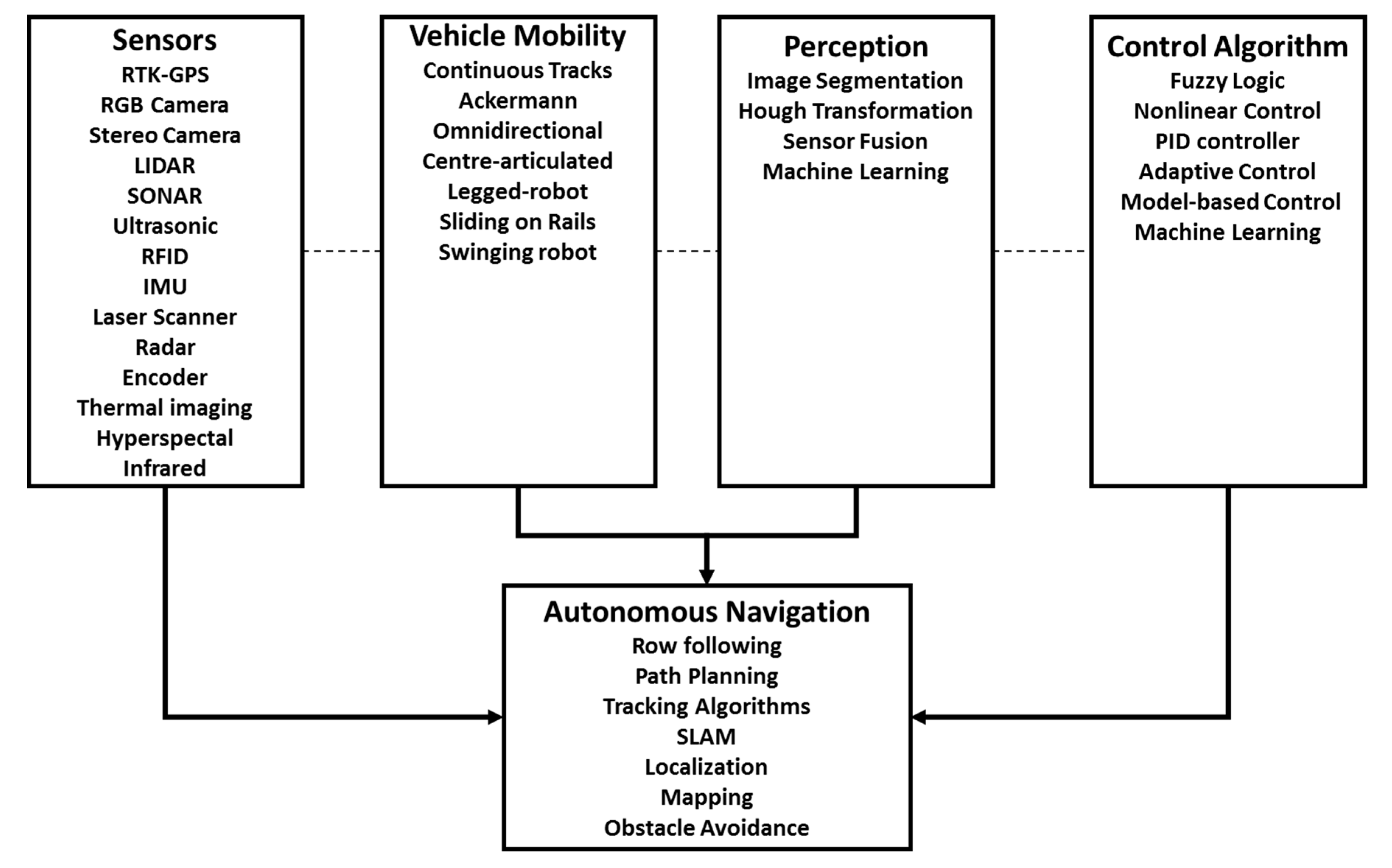
1. Introduction
- Development of the navigation system of the autonomous center-articulated hydrostatic transmission MPR.
- Evaluation of the navigation of the autonomous center-articulated hydrostatic drive MPR in a cotton field.
2. Materials and Methods
2.1. Robot Components and System Setup
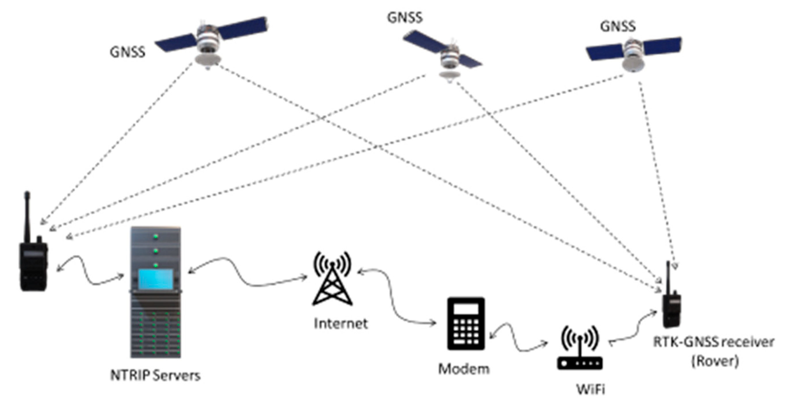
2.2. Real-Time Kinematic GNSS and Network Transport of Radio Technical Commission for Maritime Services (RTCM) via Internet Protocol (NTRIP)
2.3. Calibration of the Potentiometer, IMUs, and Encoders
| Algorithm 1: Proportional control of the articulation angle. |
| Input: Angle reported by the high precision potentiometer γk , target angle γk+1 and threshold Et Output: p which is equal to Kp* (γk+1 - γk)
|
2.4. Robot Navigation Systems
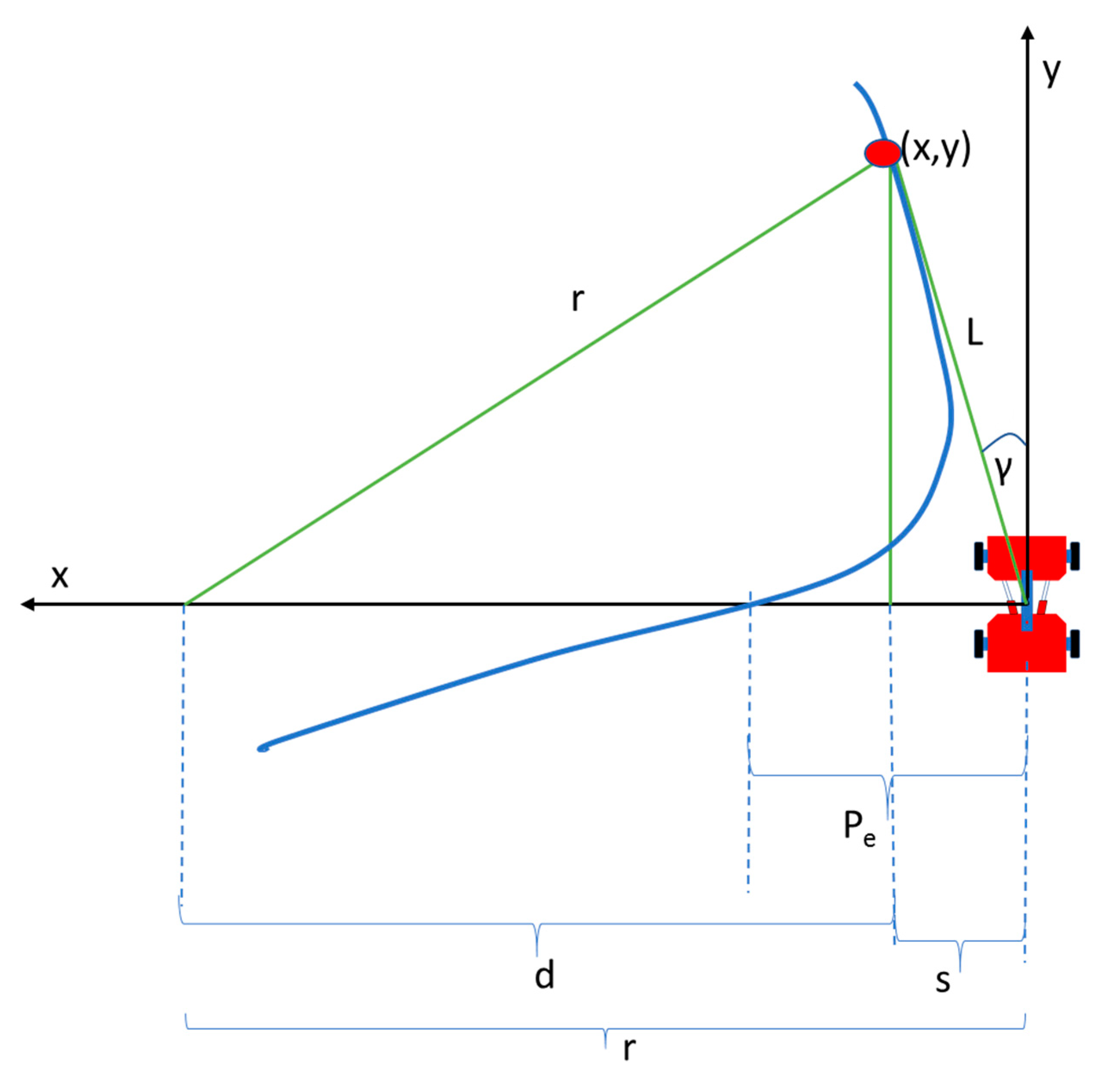
2.5. Modified Pure Pursuit
x = s
x2 + y2 = L2
2.6. Proportional Control of the Articulation Angle
2.7. Proportional Control of the Speed of the Rover
2.8. Waypoints Collection and Cubic Spline Interpolation of the Waypoints
| Algorithm 2: Cubic Spline Algorithm to estimate subinterval of UTM waypoints data intervals. |
| Input: x0, x1, x2, …, xn; a0 = f(x0), a1 = f(x1), a2 = f(x2), ….. an = f(xn) Output: ai, bi, ci, di for j = 0,1,2,…..,n-1
|
2.9. Preliminary Experiment
- A fast ROS rate was set to 10 Hz;
- A short look ahead was set at 1 m;
- Path error was set to 0 which means K x Pe = 0;
- An optimal condition was set (long look-ahead is 3 m, path error is 1.5 times path error and slow ROS rate at 1 Hz).
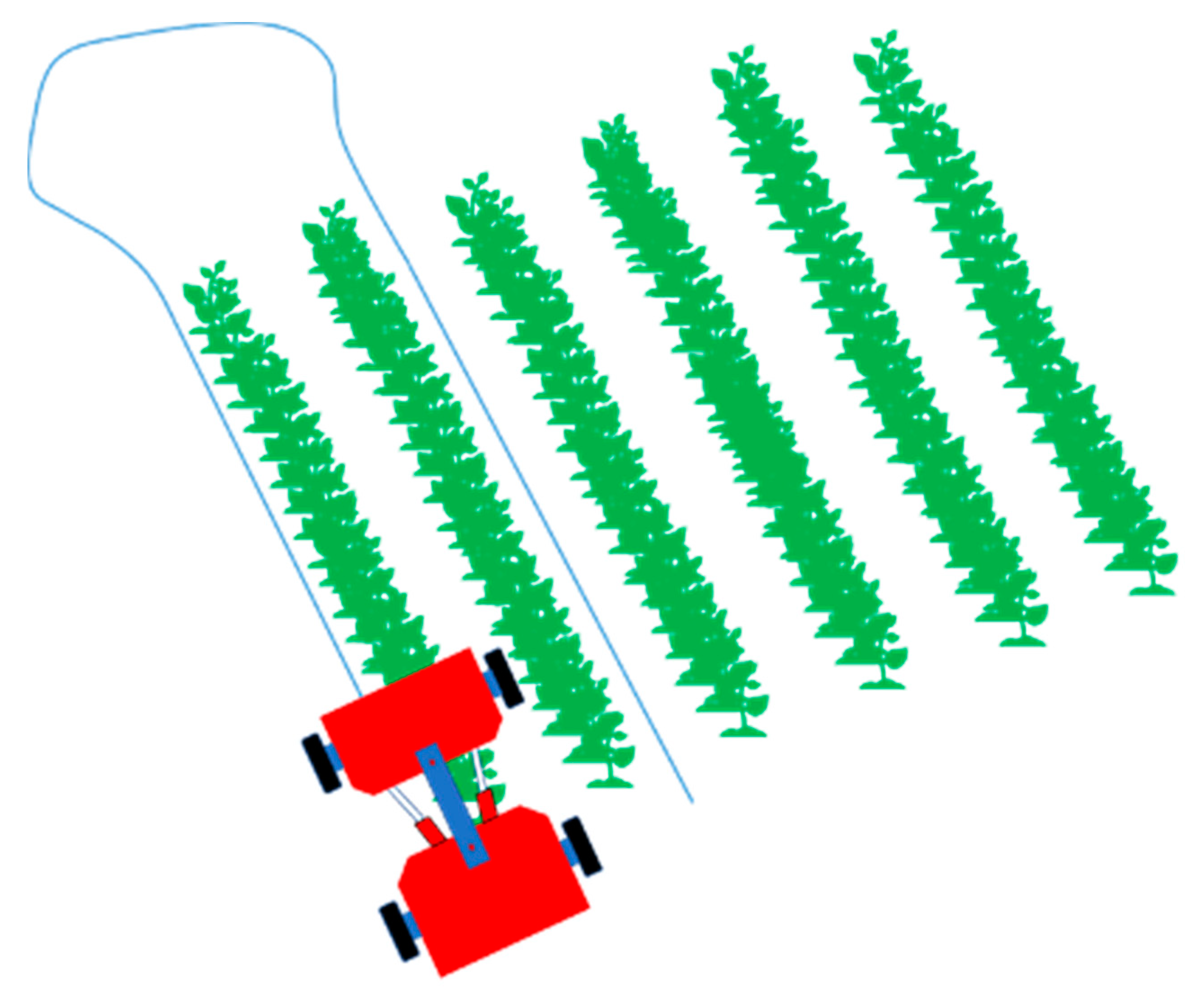
2.10. Field Experiment
3. Results and Discussions
3.1. Preliminary Experiment
3.2. Field Experiments
4. Conclusions
Author Contributions
Funding
Acknowledgments
Conflicts of Interest
References
- Hayes, L. Those Cotton Picking Robots. 2017. Available online: http://georgia.growingamerica.com/features/2017/08/those-cotton-picking-robots (accessed on 29 August 2019).
- Fue, K.G.; Porter, W.M.; Rains, G.C. Real-Time 3D Measurement of Cotton Boll Positions Using Machine Vision Under Field Conditions. In Proceedings of the 2018 BWCC, San Antonio, TX, USA, 3–5 January 2018; pp. 43–54. [Google Scholar]
- UGA Cotton News. 2019 Georgia Cotton Production Guide; U.E. Team, Ed.; UGA Extension Team: Tifton, GA, USA, 2019. [Google Scholar]
- USDA/NASS. 2017 State Agriculture Overview for Georgia. 2018. Available online: https://www.nass.usda.gov/Quick_Stats/Ag_Overview/stateOverview.php?state=GEORGIA (accessed on 29 August 2019).
- Duckett, T.; Pearson, S.; Blackmore, S.; Grieve, B.; Chen, W.-H.; Cielniak, G.; Cleaversmith, J.; Dai, J.; Davis, S.; Fox, C.; et al. Agricultural robotics: The future of robotic agriculture. arXiv 2018, arXiv:1806.06762. [Google Scholar]
- Rains, G.C.; Faircloth, A.G.; Thai, C.; Raper, R.L. Evaluation of a simple pure pursuit path-following algorithm for an autonomous, articulated-steer vehicle. Appl. Eng. Agric. 2014, 30, 367–374. [Google Scholar]
- Fue, K.G.; Porter, W.M.; Barnes, E.M.; Rains, G.C. An Extensive Review of Mobile Agricultural Robotics for Field Operations: Focus on Cotton Harvesting. Agric. Eng. 2020, 2, 10. [Google Scholar] [CrossRef]
- Reiser, D.; Sehsah, E.-S.; Bumann, O.; Morhard, J.; Griepentrog, H.W. Development of an Autonomous Electric Robot Implement for Intra-Row Weeding in Vineyards. Agriculture 2019, 9, 18. [Google Scholar] [CrossRef]
- Auat Cheein, F.; Steiner, G.; Perez Paina, G.; Carelli, R. Optimized EIF-SLAM algorithm for precision agriculture mapping based on stems detection. Comput. Electron. Agric. 2011, 78, 195–207. [Google Scholar] [CrossRef]
- Cheein, F.A.A.; Carelli, R.; Cruz, C.D.L.; Bastos-Filho, T.F. SLAM-based turning strategy in restricted environments for car-like mobile robots. In Proceedings of the 2010 IEEE International Conference on Industrial Technology, Vina del Mar, Chile, 14–17 March 2010. [Google Scholar]
- Ouadah, N.; Ourak, L.; Boudjema, F. Car-Like Mobile Robot Oriented Positioning by Fuzzy Controllers. Int. J. Adv. Robot. Syst. 2008, 5, 25. [Google Scholar] [CrossRef]
- Higuti, V.A.H.; Velasquez, A.E.B.; Magalhaes, D.V.; Becker, M.; Chowdhary, G. Under canopy light detection and ranging-based autonomous navigation. J. Field Robot. 2019, 36, 547–567. [Google Scholar] [CrossRef]
- Xue, J.; Zhang, L.; Grift, T.E. Variable field-of-view machine vision based row guidance of an agricultural robot. Comput. Electron. Agric. 2012, 84, 85–91. [Google Scholar] [CrossRef]
- Farzan, S.; Hu, A.-P.; Davies, E.; Rogers, J. Modeling and control of brachiating robots traversing flexible cables. In Proceedings of the 2018 IEEE International Conference on Robotics and Automation (ICRA), Brisbane, Australia, 21–25 May 2018. [Google Scholar]
- Grimstad, L.; From, P.J. The Thorvald II Agricultural Robotic System. Robotics 2017, 6, 24. [Google Scholar] [CrossRef]
- Xiong, Y.; Peng, C.; Grimstad, L.; From, P.J.; Isler, V. Development and field evaluation of a strawberry harvesting robot with a cable-driven gripper. Comput. Electron. Agric. 2019, 157, 392–402. [Google Scholar] [CrossRef]
- Ramin Shamshiri, R.; Weltzien, C.; Hameed, I.A.; Yule, I.J.; Grift, T.E.; Balasundram, S.K.; Pitonakova, L.; Ahmad, D.; Chowdhary, G. Research and development in agricultural robotics: A perspective of digital farming. Int. J. Agric. Biol. Eng. 2018, 11, 1–11. [Google Scholar] [CrossRef]
- Ball, D.; Upcroft, B.; Wyeth, G.; Corke, P.; English, A.; Ross, P.; Patten, T.; Fitch, R.; Sukkarieh, S.; Bate, A. Vision-based obstacle detection and navigation for an agricultural robot. J. Field Robot. 2016, 33, 1107–1130. [Google Scholar] [CrossRef]
- Kayacan, E.; Kayacan, E.; Chen, I.M.; Ramon, H.; Saeys, W. On the comparison of model-based and model-free controllers in guidance, navigation and control of agricultural vehicles. In Type-2 Fuzzy Logic and Systems; John, R., Hagras, H., Castillo, O., Eds.; Springer: Berlin/Heidelberg, Germany, 2018; pp. 49–73. [Google Scholar]
- Tu, X.; Gai, J.; Tang, L. Robust navigation control of a 4WD/4WS agricultural robotic vehicle. Comput. Electron. Agric. 2019, 164, 104892. [Google Scholar] [CrossRef]
- Boubin, J.; Chumley, J.; Stewart, C.; Khanal, S. Autonomic computing challenges in fully autonomous precision agriculture. In Proceedings of the 2019 IEEE International Conference on Autonomic Computing (ICAC), Umea, Sweden, 16–20 June 2019. [Google Scholar]
- Wang, H.; Noguchi, N. Adaptive turning control for an agricultural robot tractor. Int. J. Agric. Biol. Eng. 2018, 11, 113–119. [Google Scholar] [CrossRef]
- Liakos, G.K.; Busato, P.; Moshou, D.; Pearson, S.; Bochtis, D. Machine Learning in Agriculture: A Review. Sensors 2018, 18, 2674. [Google Scholar] [CrossRef] [PubMed]
- Coulter, R.C. Implementation of the Pure Pursuit Path Tracking Algorithm; Technical Report; Defense Technical Information Center: Fort Belvoir, VA, USA, 1 January 1992. [Google Scholar]
- Backman, J.; Oksanen, T.; Visala, A. Navigation system for agricultural machines: Nonlinear model predictive path tracking. Comput. Electron. Agric. 2012, 82, 32–43. [Google Scholar] [CrossRef]
- Gupta, N.; Khosravy, M.; Gupta, S.; Dey, N.; Crespo, R.G. Lightweight Artificial Intelligence Technology for Health Diagnosis of Agriculture Vehicles: Parallel Evolving Artificial Neural Networks by Genetic Algorithm. Int. J. Parallel Program 2020, 1–26. [Google Scholar] [CrossRef]
- Fulop, A.-O.; Tamas, L. Lessons learned from lightweight CNN based object recognition for mobile robots. In Proceedings of the 2018 IEEE International Conference on Automation, Quality and Testing, Robotics (AQTR), Cluj-Napoca, Romania, 24–26 May 2018. [Google Scholar]
- Chennoufi, M.; Bendella, F.; Bouzid, M. Multi-agent simulation collision avoidance of complex system: Application to evacuation crowd behavior. Int. J. Ambient. Comput. Intell. 2018, 9, 43–59. [Google Scholar]
- Vougioukas, S.G. A distributed control framework for motion coordination of teams of autonomous agricultural vehicles. Biosyst. Eng. 2012, 113, 284–297. [Google Scholar] [CrossRef]
- Jasiński, M.; Mączak, J.; Szulim, P.; Radkowski, S. Autonomous agricultural robot-collision avoidance methods overview. Zesz. Nauk. Inst. PojazdóW 2016, 2, 37–44. [Google Scholar]
- Gupta, S.; Khosravy, M.; Gupta, N.; Darbari, H.; Patel, N. Hydraulic system onboard monitoring and fault diagnostic in agricultural machine. Braz. Arch. Biol. Technol. 2019, 62, 1–15. [Google Scholar] [CrossRef]
- Gupta, S.; Khosravy, M.; Gupta, N.; Darbari, H. In-field failure assessment of tractor hydraulic system operation via pseudospectrum of acoustic measurements. Turk. J. Electr. Eng. Comput. Sci. 2019, 27, 2718–2729. [Google Scholar] [CrossRef]
- Gupta, N.; Khosravy, M.; Patel, N.; Dey, N.; Gupta, S.; Darbari, H.; Crespo, R.G. Economic data analytic AI technique on IoT edge devices for health monitoring of agriculture machines. Appl. Intell. 2020, 1–27. [Google Scholar] [CrossRef]
- Carpio, R.F.; Potena, C.; Maiolini, J.; Ulivi, G.; Rosselló, N.B.; Garone, E.; Gasparri, A. A Navigation Architecture for Ackermann Vehicles in Precision Farming. IEEE Robot. Autom. Lett. 2020, 5, 1103–1110. [Google Scholar] [CrossRef]
- Gao, X.; Li, J.; Fan, L.; Zhou, Q.; Yin, K.; Wang, J.; Song, C.; Huang, L.; Wang, Z. Review of Wheeled Mobile Robots’ Navigation Problems and Application Prospects in Agriculture. IEEE Access 2018, 6, 49248–49268. [Google Scholar] [CrossRef]
- Gao, Y.; Cao, D.; Shen, Y. Path-following control by dynamic virtual terrain field for articulated steer vehicles. Veh. Syst. Dyn. 2019, 1–25. [Google Scholar] [CrossRef]
- Koubâa, A. Robot Operating System (ROS); Springer: Berlin/Heidelberg, Germany, 2017. [Google Scholar]
- Quigley, M.; Conley, K.; Gerkey, B.; Faust, J.; Foote, T.; Leibs, J.; Wheeler, R.; Ng, A.Y. ROS: An open-source Robot Operating System. In Proceedings of the ICRA Workshop on Open Source Software, Kobe, Japan, 12–17 May 2009. [Google Scholar]
- Samuel, M.; Hussein, M.; Mohamad, M.B. A review of some pure-pursuit based path tracking techniques for control of autonomous vehicle. Int. J. Comput. Appl. 2016, 135, 35–38. [Google Scholar] [CrossRef]
- Bergerman, M.; Billingsley, J.; Reid, J.; van Henten, E. Robotics in Agriculture and Forestry. In Springer Handbook of Robotics; Siciliano, B., Khatib, O., Eds.; Springer: Berlin/Heidelberg, Germany, 2016; pp. 1065–1077. [Google Scholar]
- Botterill, T.; Paulin, S.; Green, R.; Williams, S.; Lin, J.; Saxton, V.; Mills, S.; Chen, X.; Corbett-Davies, S. A Robot System for Pruning Grape Vines. J. Field Robot. 2017, 34, 1100–1122. [Google Scholar] [CrossRef]
- Wan, E.A.; Nelson, A.T. Dual extended Kalman filter methods. Kalman Filter. Neural Networks 2001, 123, 123–173. [Google Scholar]
- Moore, T.; Stouch, D. A generalized extended kalman filter implementation for the robot operating system. In Intelligent Autonomous Systems; Strand, M., Dillmann, R., Menegatti, E., Ghidoni, S., Eds.; Springer: Berlin/Heidelberg, Germany, 2016; pp. 335–348. [Google Scholar]
- Post, M.A.; Bianco, A.; Yan, X.T. Autonomous navigation with ROS for a mobile robot in agricultural fields. In Proceedings of the 14th International Conference on Informatics in Control, Automation and Robotics (ICINCO), Madrid, Spain, 26–28 July 2017. [Google Scholar]
- Corke, P.I.; Ridley, P. Steering kinematics for a center-articulated mobile robot. IEEE Trans. Robot. Autom. 2001, 17, 215–218. [Google Scholar] [CrossRef]
- Oberhammer, J.; Tang, M.; Liu, A.-Q.; Stemme, G. Mechanically tri-stable, true single-pole-double-throw (SPDT) switches. J. Micromech. Microeng. 2006, 16, 2251. [Google Scholar] [CrossRef]
- McKinley, S.; Levine, M. Cubic spline interpolation. Coll. Redwoods 1998, 45, 1049–1060. [Google Scholar]


| Mean ± Std. Dev (m) | 1st Pass | 2nd Pass | 3rd Pass | Overall |
|---|---|---|---|---|
| 1St Row | 0.048 ± 0.036 | 0.048 ± 0.035 | 0.066 ± 0.0046 | 0.053 ± 0.041 |
| Turning | 0.233 ± 0.198 | 0.227 ± 0.211 | 0.244 ± 0.211 | 0.235 ± 0.206 |
| 2nd Row | 0.036 ± 0.024 | 0.081 ± 0.028 | 0.115 ± 0.043 | 0.070 ± 0.046 |
| Overall (1st and 2nd Rows) | 0.042 ± 0.032 | 0.062 ± 0.036 | 0.091 ± 0.053 | 0.061 ± 0.044 |
© 2020 by the authors. Licensee MDPI, Basel, Switzerland. This article is an open access article distributed under the terms and conditions of the Creative Commons Attribution (CC BY) license (http://creativecommons.org/licenses/by/4.0/).
Share and Cite
Fue, K.; Porter, W.; Barnes, E.; Li, C.; Rains, G. Autonomous Navigation of a Center-Articulated and Hydrostatic Transmission Rover using a Modified Pure Pursuit Algorithm in a Cotton Field. Sensors 2020, 20, 4412. https://doi.org/10.3390/s20164412
Fue K, Porter W, Barnes E, Li C, Rains G. Autonomous Navigation of a Center-Articulated and Hydrostatic Transmission Rover using a Modified Pure Pursuit Algorithm in a Cotton Field. Sensors. 2020; 20(16):4412. https://doi.org/10.3390/s20164412
Chicago/Turabian StyleFue, Kadeghe, Wesley Porter, Edward Barnes, Changying Li, and Glen Rains. 2020. "Autonomous Navigation of a Center-Articulated and Hydrostatic Transmission Rover using a Modified Pure Pursuit Algorithm in a Cotton Field" Sensors 20, no. 16: 4412. https://doi.org/10.3390/s20164412
APA StyleFue, K., Porter, W., Barnes, E., Li, C., & Rains, G. (2020). Autonomous Navigation of a Center-Articulated and Hydrostatic Transmission Rover using a Modified Pure Pursuit Algorithm in a Cotton Field. Sensors, 20(16), 4412. https://doi.org/10.3390/s20164412