The Accuracy of the Microsoft Kinect V2 Sensor for Human Gait Analysis. A Different Approach for Comparison with the Ground Truth

 ,
,  ,
,  ,
,  and
and 
Abstract
1. Introduction
2. Methods
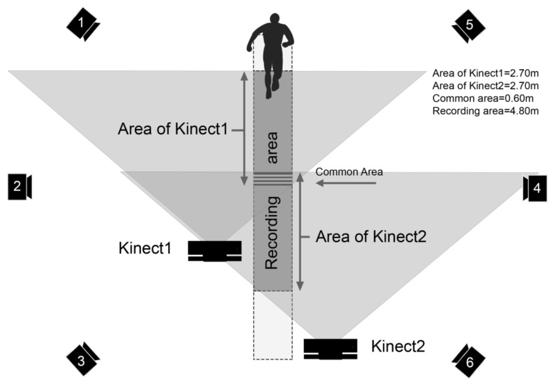
2.1. Data Collection
2.2. Data Processing
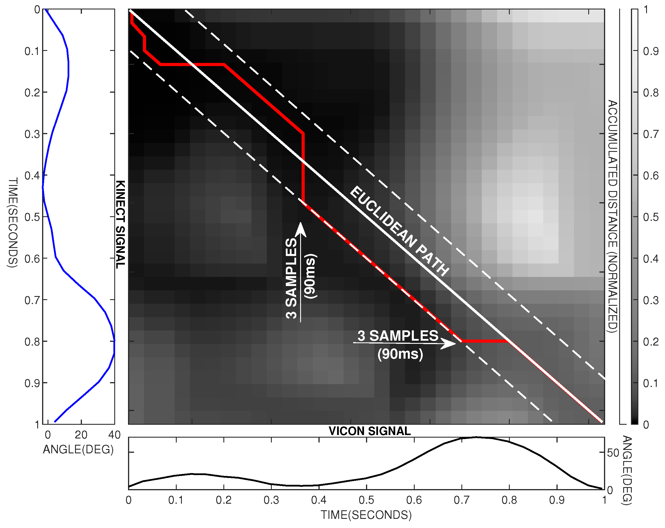
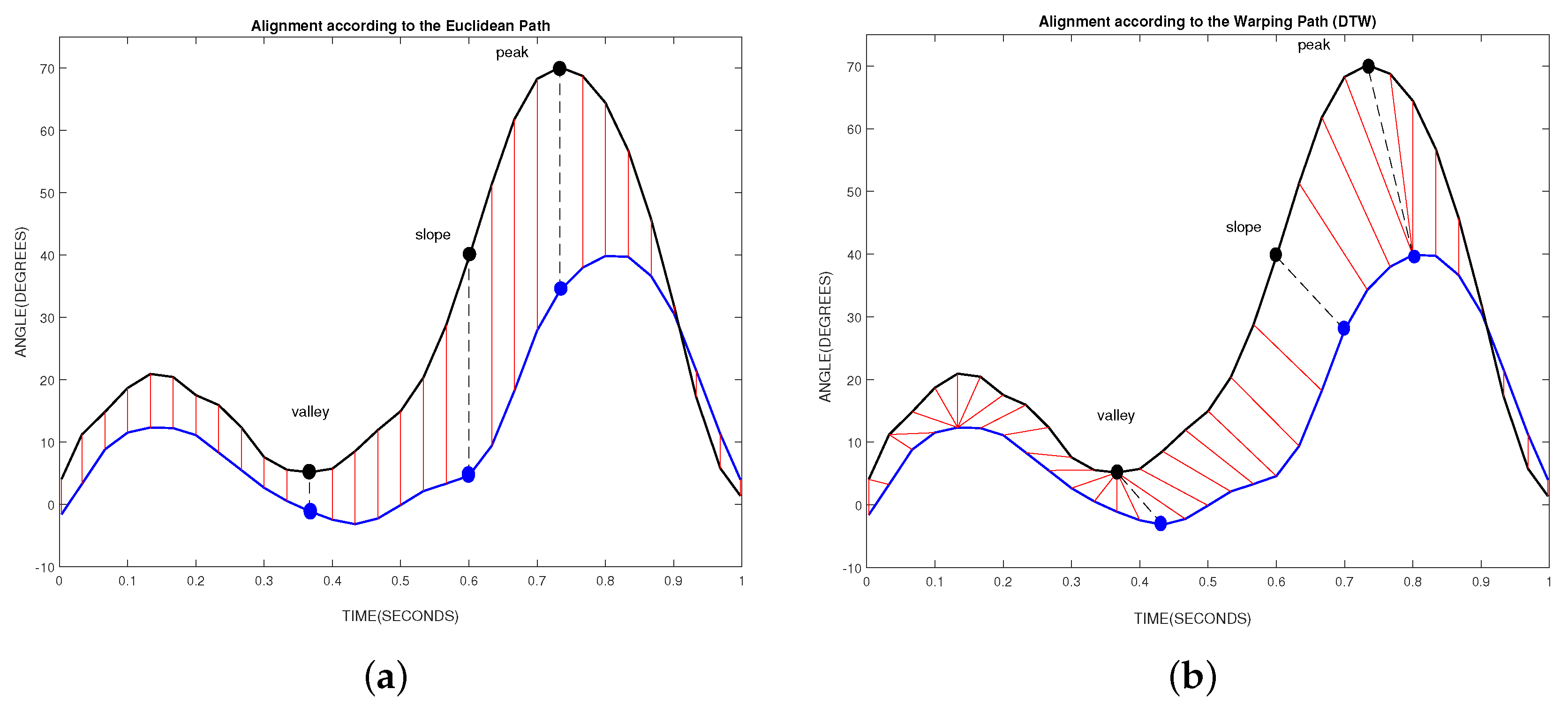
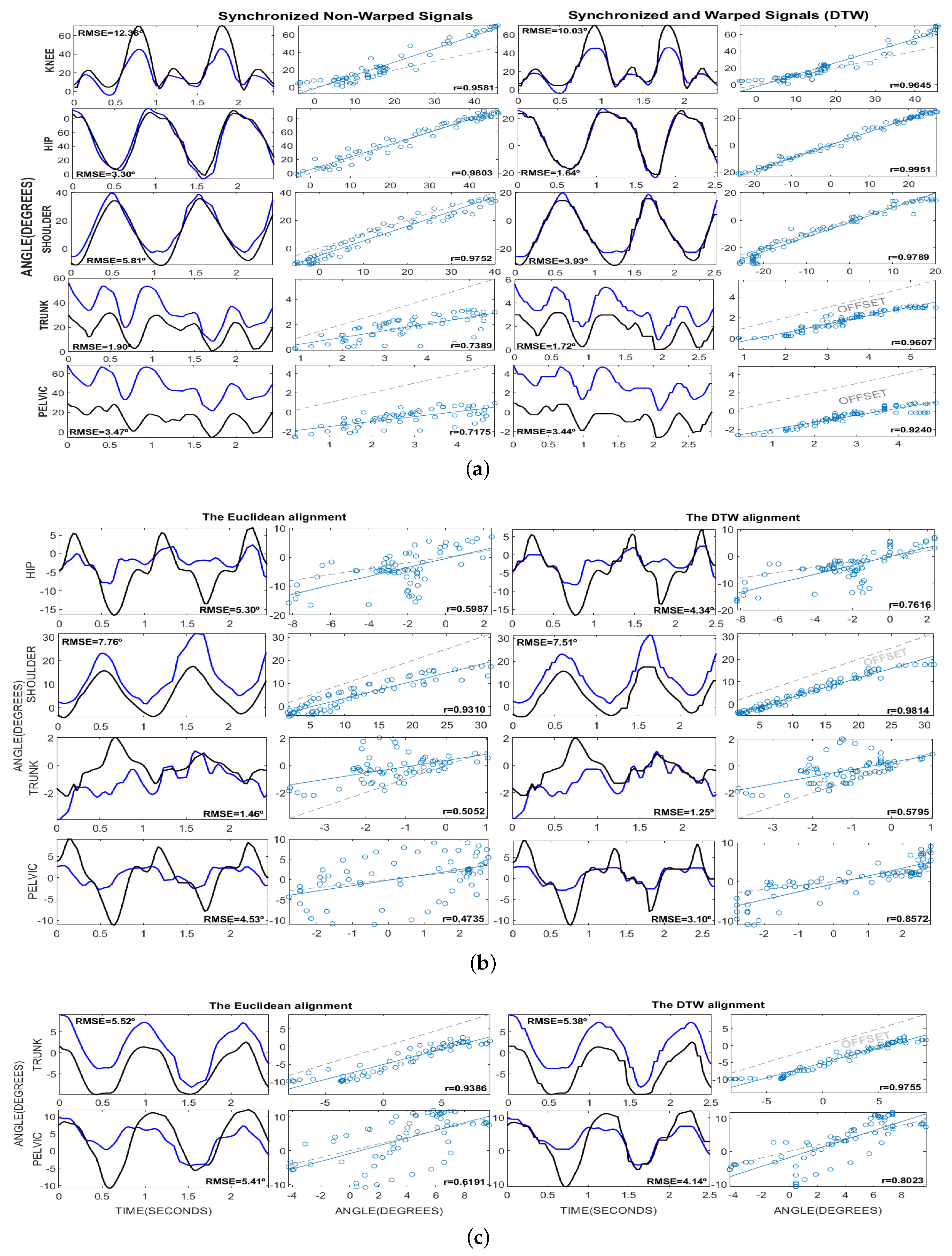
2.3. Data Analysis
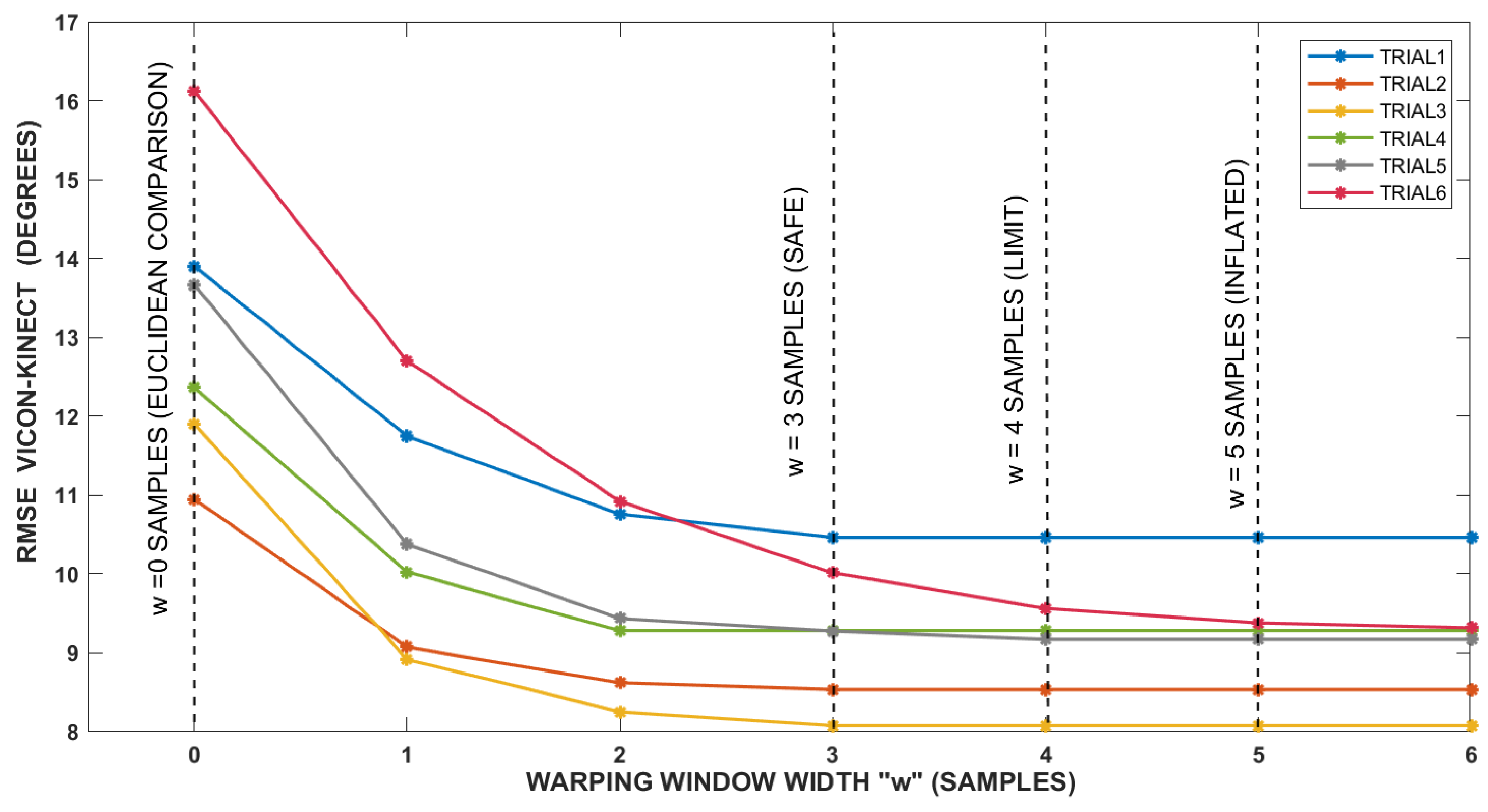
3. Results
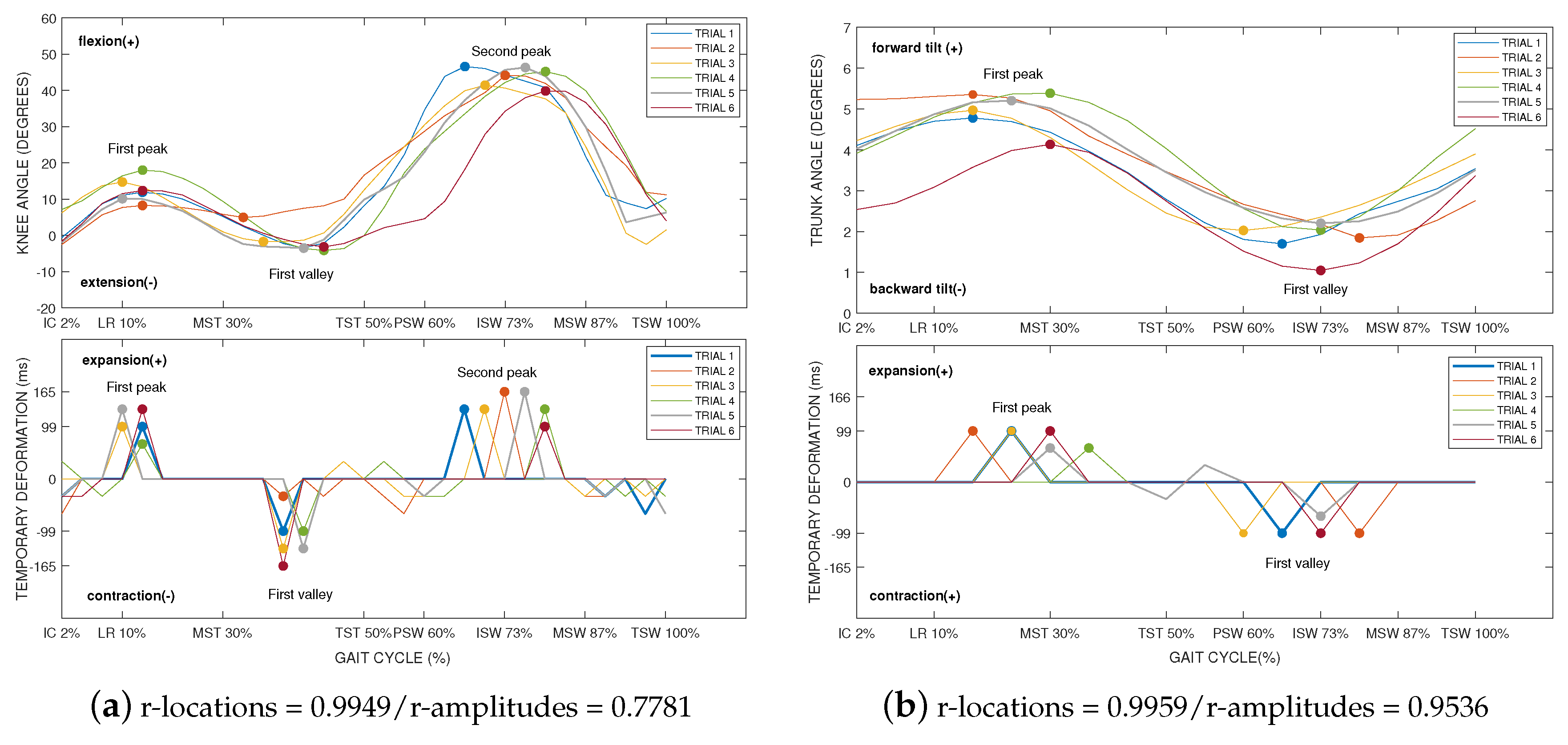
The Presence of Temporary Deformation Patterns
4. Discussion
5. Conclusions
Author Contributions
Funding
Acknowledgments
Conflicts of Interest
References
- Bilesan, A.; Behzadipour, S.; Tsujita, T.; Komizunai, S.; Konno, A. Markerless Human Motion Tracking Using Microsoft Kinect SDK and Inverse Kinematics. In Proceedings of the 2019 12th Asian Control Conference (ASCC), Kitakyushu-shi, Japan, 9–12 June 2019; pp. 504–509. [Google Scholar]
- Dolatabadi, E.; Taati, B.; Mihailidis, A. An automated classification of pathological gait using unobtrusive sensing technology. IEEE Trans. Neural Syst. Rehabil. Eng. 2017, 25, 2336–2346. [Google Scholar] [CrossRef] [PubMed]
- Springer, S.; Seligmann, G. Validity of the Kinect for Gait Assessment: A Focused Review. Sensors 2016, 16, 194. [Google Scholar] [CrossRef] [PubMed]
- Mentiplay, B.F.; Perraton, L.G.; Bower, K.J.; Pua, Y.H.; Mcgaw, R.; Heywood, S.; Clark, R.A. Gait assessment using the Microsoft Xbox One Kinect: Concurrent validity and inter-day reliability of spatiotemporal and kinematic variables. J. Biomech. 2015, 48, 2166–2170. [Google Scholar] [CrossRef] [PubMed]
- Ma, Y.; Mithraratne, K.; Wilson, N.C.; Wang, X.; Zhang, Y. The validity and reliability of a kinect v2-based gait analysis system for children with cerebral palsy. Sensors 2019, 19, 1660. [Google Scholar] [CrossRef]
- Schlagenhauf, F.; Sreeram, S.; Singhose, W. Comparison of Kinect and Vicon Motion Capture of Upper-Body Joint Angle Tracking. In Proceedings of the 2018 IEEE 14th International Conference on Control and Automation (ICCA), Anchorage, AK, USA, 12–15 June 2018; IEEE Computer Society: Piscataway, NJ, USA, 2018; Volume 2018, pp. 674–679. [Google Scholar]
- Tanaka, R.; Takimoto, H.; Yamasaki, T.; Higashi, A. Validity of time series kinematical data as measured by a markerless motion capture system on a flatland for gait assessment. J. Biomech. 2018, 71, 281–285. [Google Scholar] [CrossRef]
- Otte, K. Accuracy and Reliability of the Kinect Version 2 for Clinical Measurement of Motor Function. PLoS ONE 2016, 11, e0166532. [Google Scholar] [CrossRef]
- Livingston, M.A.; Sebastian, J.; Ai, Z.; Decker, J.W. Performance measurements for the Microsoft Kinect skeleton. In Proceedings of the 2012 IEEE Virtual Reality Workshops (VRW), Costa Mesa, CA, USA, 4–8 March 2012; IEEE: Piscataway, NJ, USA, 2012; pp. 119–120. [Google Scholar]
- Webster, D.; Celik, O. Experimental evaluation of Microsoft Kinect’s accuracy and capture rate for stroke rehabilitation applications. In Proceedings of the2014 IEEE Haptics Symposium (HAPTICS), Houston, TX, USA, 23–26 February 2014; IEEE Computer Society: Piscataway, NJ, USA, 2014; pp. 455–460. [Google Scholar]
- Edwards, M.; Green, R. Low-Latency Filtering of Kinect Skeleton Data for Video Game Control. In Proceedings of the 29th International Conference on Image and Vision Computing New Zealand, IVCNZ’14, Hamilton, New Zealand, 19–21 November 2014; Volume 19–21, pp. 190–195. [Google Scholar]
- Guess, T.M. Comparison of 3D Joint Angles Measured With the Kinect 2.0 Skeletal Tracker Versus a Marker-Based Motion Capture System. J. Appl. Biomech. 2017, 33, 176–182. [Google Scholar] [CrossRef]
- Pohl, M.B.; Messenger, N.; Buckley, J.G. Changes in foot and lower limb coupling due to systematic variations in step width. Clin. Biomech. 2006, 21, 175–183. [Google Scholar] [CrossRef]
- Chan, J.; Leung, H.; Poizner, H. Correlation Among Joint Motions Allows Classification of Parkinsonian Versus Normal 3-D Reaching. IEEE Trans. Neural Syst. Rehabil. Eng. 2010, 18, 142–149. [Google Scholar] [CrossRef][Green Version]
- Park, K.; Dankowicz, H.; Hsiao-Wecksler, E.T. Characterization of spatiotemporally complex gait patterns using cross-correlation signatures. Gait Posture 2012, 36, 120–126. [Google Scholar] [CrossRef]
- Sakoe, H.; Chiba, S. Dynamic programming algorithm optimization for spoken word recognition. IEEE Trans. Acoust. 1978, 26, 43–49. [Google Scholar] [CrossRef]
- Boulgouris, N.V.; Plataniotis, K.N.; Hatzinakos, D. Gait recognition using dynamic time warping. In Proceedings of the IEEE 6th Workshop on Multimedia Signal Processing, Siena, Italy, 29 September–1 October 2004; IEEE: Piscataway, NJ, USA, 2004; pp. 263–266. [Google Scholar]
- Patras, L.; Giosan, I.; Nedevschi, S. Body gesture validation using multi-dimensional dynamic time warping on Kinect data. In Proceedings of the 2015 IEEE International Conference on Intelligent Computer Communication and Processing (ICCP), Cluj-Napoca, Romania, 3–5 September 2015; IEEE: Piscataway, NJ, USA, 2015; pp. 301–307. [Google Scholar]
- Gaspar, M.; Welke, B.; Seehaus, F.; Hurschler, C.; Schwarze, M. Dynamic Time Warping compared to established methods for validation of musculoskeletal models. J. Biomech. 2017, 55, 156–161. [Google Scholar] [CrossRef] [PubMed]
- Mueen, A.; Keogh, E. Extracting Optimal Performance from Dynamic Time Warping. In Proceedings of the 22nd ACM SIGKDD International Conference on Knowledge Discovery and Data Mining, KDD’16, San Francisco, CA, USA, 13–17 August 2016; Volume 13–17, pp. 2129–2130. [Google Scholar]
- Shi, L.; Duan, F.; Yang, Y.; Sun, Z. The Effect of Treadmill Walking on Gait and Upper Trunk through Linear and Nonlinear Analysis Methods. Sensors 2019, 19, 2204. [Google Scholar] [CrossRef] [PubMed]
- Kharazi, M.R.; Memari, A.H.; Shahrokhi, A.; Nabavi, H.; Khorami, S.; Rasooli, A.H.; Barnamei, H.R.; Jamshidian, A.R.; Mirbagheri, M.M. Validity of microsoft kinectTM for measuring gait parameters. In Proceedings of the 2015 22nd Iranian Conference on Biomedical Engineering (ICBME), Tehran, Iran, 25–27 November 2015; IEEE: Piscataway, NJ, USA, 2015; pp. 375–379. [Google Scholar]
- Pfister, A.; West, A.M.; Bronner, S.; Noah, J.A. Comparative abilities of Microsoft Kinect and Vicon 3D motion capture for gait analysis. J. Med. Eng. Technol. 2014, 38, 274–280. [Google Scholar] [CrossRef] [PubMed]
- Bravo, M.D.A.; Rengifo, R.C.F.; Agredo, R.W. Comparación de dos Sistemas de Captura de Movimiento por medio de las Trayectorias Articulares de Marcha. Rev. Mex. Ing. Biomed. 2016, 37, 149–160. [Google Scholar]
- Guffanti, D.; Brunete, A.; Hernando, M. Non-Invasive Multi-Camera Gait Analysis System and its Application to Gender Classification. IEEE Access 2020, 8, 95734–95746. [Google Scholar] [CrossRef]
- Ma, M.; Proffitt, R.; Skubic, M.; Jan, Y.K. Validation of a Kinect V2 based rehabilitation game. PLoS ONE 2018, 13, e0202338. [Google Scholar] [CrossRef]
- Wei, T.; Lee, B.; Qiao, Y.; Kitsikidis, A.; Dimitropoulos, K.; Grammalidis, N. Experimental study of skeleton tracking abilities from microsoft kinect non-frontal views. In Proceedings of the 2015 3DTV-Conference: The True Vision—Capture, Transmission and Display of 3D Video (3DTV-CON), Lisbon, Portugal, 8–10 July 2015; IEEE: Piscataway, NJ, USA, 2015; Volume 2015, pp. 1–4. [Google Scholar]
- Davis, R.B.; Õunpuu, S.; Tyburski, D.; Gage, J.R. A gait analysis data collection and reduction technique. Hum. Mov. Sci. 1991, 10, 575–587. [Google Scholar] [CrossRef]
- Ceccato, J.C.; de Sèze, M.; Azevedo, C.; Cazalets, J.R. Comparison of Trunk Activity during Gait Initiation and Walking in Humans (Trunk Activity in Walking). PLoS ONE 2009, 4, e8193. [Google Scholar] [CrossRef]
- Keogh, E.; Ratanamahatana, C.A. Exact indexing of dynamic time warping. Knowl. Inf. Syst. 2005, 7, 358–386. [Google Scholar] [CrossRef]
- Górecki, T.; Łuczak, M. The influence of the Sakoe-Chiba band size on time series classification. J. Intell. Fuzzy Syst. 2019, 36, 527–539. [Google Scholar] [CrossRef]
- Vidal Ruiz, E.; Casacuberta Nolla, F.; Rulot Segovia, H. Is the DTW “distance” really a metric? An algorithm reducing the number of DTW comparisons in isolated word recognition. Speech Commun. 1985, 4, 333–344. [Google Scholar] [CrossRef]


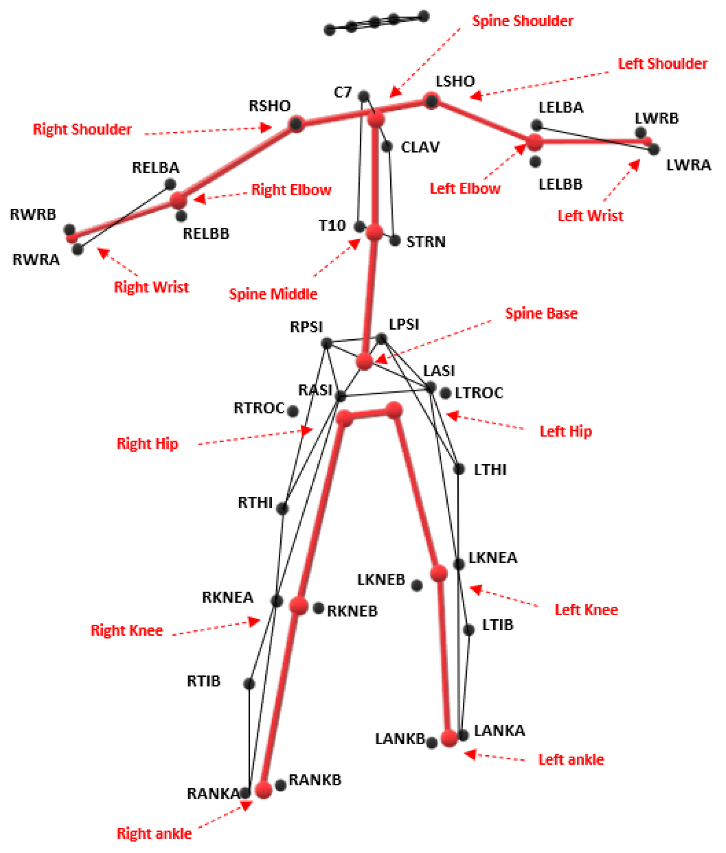
| Kinect V2 Equivalent Joint | Vicon Markers |
|---|---|
| Spine base | Midpoint [RPSI,LPSI,RASI,LASI] |
| Spine middle | Midpoint [T10,STRN] |
| Spine shoulder | Midpoint [C7,CLAV] |
| Left shoulder | Marker LSHO |
| Left elbow | Midpoint [LELB marker A,LELB marker B] |
| Left wrist | Midpoint [LWR marker A,LWR marker B] |
| Right shoulder | Marker RSHO |
| Right elbow | Midpoint [RELB marker A,RELB marker B] |
| Right wrist | Midpoint [RWR marker A,RWR marker B] |
| Left hip | Hip joint centering algorithm [LASI,LPSI] |
| Left knee | Midpoint [LKNE marker A,LKNE marker B] |
| Left ankle | Midpoint [LANK marker A,LANK marker B] |
| Right hip | Hip joint centering algorithm [RASI,RPSI] |
| Right knee | Midpoint [RKNE marker A,RKNE marker B] |
| Right ankle | Midpoint [RANK marker A,RANK marker B] |
| Euclidean Matching | Dynamic Time Warping Matching | ||||||
|---|---|---|---|---|---|---|---|
| RMSE (°) | Pearson Correlation | Qualitative r | RMSE (°) | Pearson Correlation | Qualitative r | ||
| (Mean ± SD) | (Mean ± SD) | (H./M./L.) | (Mean ± SD) | (Mean ± SD) | (H./M./L.) | ||
| Sagittal | Knee flex/ext. | 13.15 ± 1.83 | 0.91 ± 0.04 | HIGH | 10.47 ± 1.49 | 0.94 ± 0.02 | HIGH |
| Hip flex/ext. | 6.20 ± 2.08 | 0.94 ± 0.03 | HIGH | 2.65 ± 1.06 | 0.99 ± 0.01 | HIGH | |
| Shoulder flex/ext. | 9.53 ± 3.88 | 0.94 ± 0.02 | HIGH | 5.80 ± 3.39 | 0.97 ± 0.03 | HIGH | |
| Trunk forw/back. tilt | 2.09 ± 0.38 | 0.75 ± 0.02 | MODERATE | 1.93 ± 0.40 | 0.91 ± 0.04 | HIGH | |
| Pelvis ant/post. tilt | 3.22 ± 0.37 | 0.72 ± 0.07 | MODERATE | 3.14 ± 0.39 | 0.87 ± 0.06 | HIGH | |
| Frontal | Hip add/abd. | 5.83 ± 0.99 | 0.41 ± 0.19 | LOW | 4.70 ± 0.94 | 0.63 ± 0.13 | MODERATE |
| Shoulder add./abd. | 11.76 ± 3.98 | 0.87 ± 0.08 | HIGH | 11.69 ± 3.98 | 0.94 ± 0.05 | HIGH | |
| Trunk right/left sway | 1.31 ± 0.39 | 0.50 ± 0.19 | MODERATE | 1.10 ± 0.36 | 0.62 ± 0.18 | MODERATE | |
| Pelvis up/down. obliquity | 4.44 ± 0.48 | 0.40 ± 0.15 | LOW | 3.11 ± 0.42 | 0.76 ± 0.08 | MODERATE | |
| Transverse | Trunk int/ext. rotation | 5.26 ± 0.64 | 0.88 ± 0.05 | HIGH | 5.09 ± 0.58 | 0.96 ± 0.02 | HIGH |
| Pelvis int/ext. rotation | 5.88 ± 0.36 | 0.54 ± 0.14 | MODERATE | 4.81 ± 0.43 | 0.72 ± 0.12 | MODERATE | |
© 2020 by the authors. Licensee MDPI, Basel, Switzerland. This article is an open access article distributed under the terms and conditions of the Creative Commons Attribution (CC BY) license (http://creativecommons.org/licenses/by/4.0/).
Share and Cite
Guffanti, D.; Brunete, A.; Hernando, M.; Rueda, J.; Navarro Cabello, E. The Accuracy of the Microsoft Kinect V2 Sensor for Human Gait Analysis. A Different Approach for Comparison with the Ground Truth. Sensors 2020, 20, 4405. https://doi.org/10.3390/s20164405
Guffanti D, Brunete A, Hernando M, Rueda J, Navarro Cabello E. The Accuracy of the Microsoft Kinect V2 Sensor for Human Gait Analysis. A Different Approach for Comparison with the Ground Truth. Sensors. 2020; 20(16):4405. https://doi.org/10.3390/s20164405
Chicago/Turabian StyleGuffanti, Diego, Alberto Brunete, Miguel Hernando, Javier Rueda, and Enrique Navarro Cabello. 2020. "The Accuracy of the Microsoft Kinect V2 Sensor for Human Gait Analysis. A Different Approach for Comparison with the Ground Truth" Sensors 20, no. 16: 4405. https://doi.org/10.3390/s20164405
APA StyleGuffanti, D., Brunete, A., Hernando, M., Rueda, J., & Navarro Cabello, E. (2020). The Accuracy of the Microsoft Kinect V2 Sensor for Human Gait Analysis. A Different Approach for Comparison with the Ground Truth. Sensors, 20(16), 4405. https://doi.org/10.3390/s20164405