1. Introduction
One of the main challenges for the safety validation of autonomous driving vehicles lies on the influence of weather phenomena [
1,
2]. As each of the main sensors, namely LIDAR, radar and cameras increases its sensitivity in order to detect smaller objects faster and hence be able to drive autonomously at higher speeds, the possible influence of environmental perturbations on their perception increases. On the one hand, those perturbations could cause false positives (the term false positives in this paper refers to a false detection in the point cloud before segmentation and classification are done), confuse self-calibration algorithms and reduce the sensor range [
3,
4]. On the other hand, they could constitute a source of valuable information if the dependencies are known and properly characterized to better evaluate and predict road conditions or adapt its operation mode, for example, [
5].
In this paper, we focus on the influence of rain, fog and snow on a LIDAR sensor. Previous results are expanded by considering not only absorption and reflection [
2] as well as changes in the reflection characteristics of the target [
3], but also the simultaneous influence of a changing ambient illumination in outdoor conditions.
With that objective in mind, a LIDAR was placed outdoors in a static position. As target, an asphalt region of a parking lot was used. The collected point cloud data was separated between detections on the atmosphere and street. The detections on those two areas were analyzed using a classifier in order to identify if, in a static scenario, reliable information about the current weather could be extracted based on the information provided by an automotive LIDAR. Finally, possible applications of the results are shown, including a way of extending the method for use in a moving platform (car/bus/truck) in which sensor and targets move. For the virtual simulation, the use of physically-based rendering is suggested in order to include the effects of a changing background illumination together with changing reflection properties of targets in a reproducible way.
The next section introduces the current state of the art regarding the influence of weather on the LIDAR performance and the use of weather classification algorithms with focus on LIDAR data.
Section 3 presents the experimental setup and
Section 4 the results for the atmosphere and street regions.
2. State of the Art
2.1. Influence of Weather on a Performance
One of the main disadvantages of optical sensors (camera and LIDAR) in comparison to radar is their higher performance degradation under the presence of rainfall, fog and snow [
6]. In general, the influence of adverse weather on the performance of a LIDAR sensor can be divided as follows:
Previous attempts to simulate the impact of weather on the performance of a LIDAR make use of the LIDAR equation [
3], which calculates the absorption and scattering coefficients of rain, snow or fog based on the drop size distribution [
12]. Given the relationship between drop size distribution and rain intensity, it is possible to use Monte Carlo simulations to calculate a false positives rate caused by the drops [
13] for a given rain intensity. Alternatively, the detections can be filtered out using a Kalman filter or dynamic radius outlier removal filters [
14,
15].
The effect of rain on the reflectance of different targets has also been studied [
2,
7]. In this case, the absorption and scattering caused by rain is characterized simultaneously with the change in target reflectance by measuring the range, intensity and number of reflected points using a LIDAR sensor for targets placed outdoors. It is found that rain causes a decrement in the intensity and number of detected points for all targets tested, which included materials such as metal, asphalt, concrete and a retro reflective surface, each one placed at a different distance [
2]. The authors mention that the change in the reflection characteristics of the target seem to generate an intensity change bigger than the one generated by absorption and scattering caused by rain [
2]. The material with the maximum reduction in number of reflected points is found to be asphalt.
This paper will focus on the case in which the LIDAR sensor and target are both placed outdoors. In that way, the effect of a changing background illumination and the change in the optical properties of the LIDARs cover are also included. As target, an asphalt portion of a parking lot is used. Besides physical effects, the influence of sensor internal algorithms that dynamically adapt the performance of the sensor like automatic gain control [
16], for example, are left active.
2.2. Effect of Water on a Surface’s Transmission and Reflection
For analysis purposes, the effect of water upon the transmission and reflection of a porous material can be divided into three stages: first, the pores of the material are filled with water. When the material reaches saturation, a thin water film forms on top of it. As the water level increases, the characteristics of the material itself lose importance and the reflection starts to depend mostly on the optical properties of water.
The first stage can be understood by considering the change in the optical path length of the material when its pores are filled with water instead of air. This implies a higher probability of absorption of the photons and hence a reduction in its transmission. Regarding reflection, the scattering of the surface changes to a more forward scattering. Consequently, as can also be seen in the visible spectral range, the surface becomes more opaque [
7]. A comparison of different dry and wet materials shows an average reflectivity reduction of around 10% for a wavelength of 900 nm and of around 30% for a wavelength of 1.5 µm [
1]
The second stage can be analyzed assuming a thin and homogenous water layer. In this case, considering the plastic cover of a LIDAR, for example, a multilayer interface is built consisting of air, plastic or glass, a coating, and a water layer. The Fresnel equations can then be used to calculate the reflectance. In most cases, though, the layer will not be homogeneous. In that case, the surface can be characterized in transmission and reflection by measuring its bidirectional transmittance distribution function (BTDF) and bidirectional reflectance distribution function (BRDF) [
17] for the required wavelength.
For further increments in the water level, the reflection can be analyzed by using the bathymetric LIDAR equation [
16].
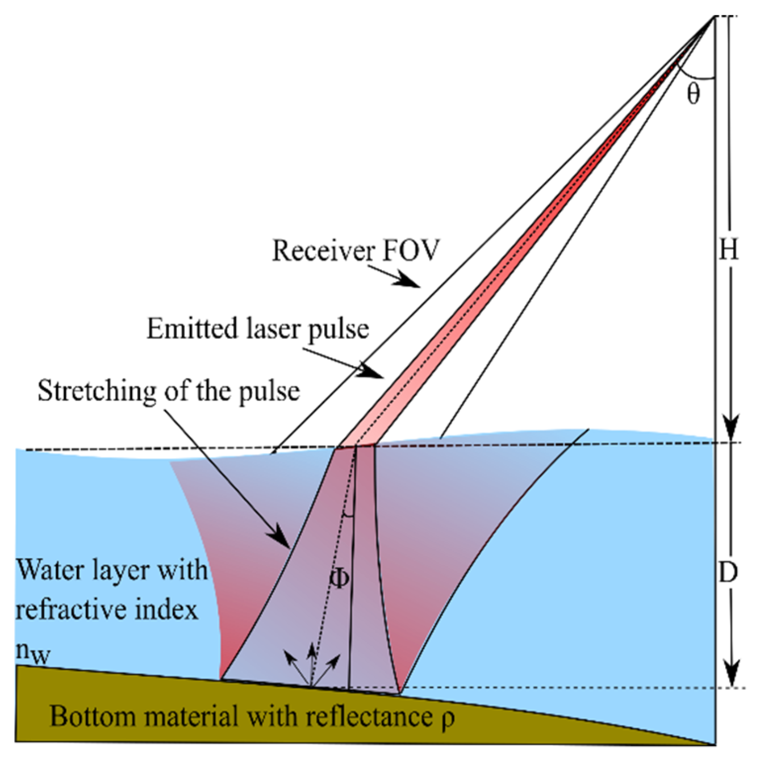
This equation uses the parameters as illustrated in
Figure 1. It is defined as:
where
corresponds to the received power,
to the transmitted power,
to the reflectance of the bottom material,
to the incident angle of the transmitted laser beam in air,
to the refracted beam angle in water,
to the altitude of the LIDAR above the water,
to the distance between the water surface and the bottom material,
the refraction index of water,
which combines stretching and attenuation of the pulse, and
is a constant containing sensor-related values [
16]. This equation corresponds to the conventional LIDAR range equation for an extended target, with an added exponential decay in a scattering medium corresponding to the Beer-Lambert law.
2.3. Effect of Ambient Light on LIDAR Measurements
Since at the end, the information obtained from the LIDAR is based on detections over the noise level, the APD (avalanche photo diode) equation also needs to be considered:
where
can be calculated as shown in Equation (1) and
corresponds to the noise which is a combination of the shot noise
, the background noise
, which is proportional to the background light optical power collected by the detector, and the thermal noise
[
1].
Finally, the time of flight (TOF) is defined as the time difference between the start of the sent pulse
and the moment when the detected intensity reaches a certain minimum value
(5). Assuming a Gaussian distribution for the noise (3), a SNR of 3
(0.27% probability that a detection is caused by noise) with respect to the mean noise level can be used, for example, in order to define a valid detection (4). If the average noise level increases from
to
as shown in
Figure 2, and the shape of the echo pulse remains the same, there is no detection. Correspondingly, the total number of reflected points is reduced. This fact is used for the analysis in the measurement section.
As can be deduced from
Figure 2 the intensity of the detection
, its distance, which is calculated using the TOF, and the EPW (Echo pulse width) value also change depending on the noise level. This kind of walk error, which can also be caused by a change in the form of the echo pulse, can in some cases be compensated but not completely avoided [
18]. The EPW, which is measured in meters [
19], corresponds to the width of the pulse above the noise level. It is proportional to the reflection of the object.
2.4. Light Scattering and Absorption by Particles in the Atmosphere
Particles in the atmosphere scatter and absorb the laser light depending on their shape, size and complex index of refraction [
20]. Spherical particles with a size parameter
smaller than 0.1 (Rayleigh regime) tend to have a symmetric forward/backwards scattering. Particles with
values between 0.1 and 50 (Mie regime) have a bigger forward as backward scattering lobe, while particles with
values bigger than 50 (Geometric regime) have a very large forward scattering lobe and almost no backwards scattering [
20]. In case of snow, the analysis is more complicated and depends on the exact shape of the crystal, which depends on the temperature [
3]. For multiple particles, the scattering coefficient is also proportional to particle concentration and size [
21].
Table 1 shows the average radius and size parameter for typical particles in the atmosphere. The size parameter is based on a laser with a wavelength of 905 nm, which is in the range of wavelengths typically used for autonomous driving cars [
22,
23]. The refractive index for both water and ice at this wavelength has an imaginary part in the order of
[
24] and hence the single scattering albedo (SSA) for both drops and crystals in the geometric regime approximates 0.53 [
25,
26]. For fog, it approximates 0.8 [
26].
Although the parameters are distributed over a broad range, not all the sizes occur with the same probability, with common sizes for snowflakes around 1 mm [
29], for rain drops around 0.2 mm and for fog droplets around 3 µm (Chu Hogg) and 18 µm (Advection) [
3].
2.5. Weather Classification Using LIDAR
There are different alternatives to evaluate current weather and road friction in the vicinity of a car. One alternative is using the information provided by the vehicle, for example from windshield wipers, fog lights, torque and speed of engine and tires, anti-lock braking system (ABS), electronic stability control (ESC) and traction control system (TCS) intervention events, temperature, global navigation satellite system (GNSS) position, steering wheel angle and breaking signal [
30]. Another alternative is to use sensors specific for road surface analysis like polarization cameras or short distance multi-wavelength IR sensors. These sensors use the change in the amount of vertically polarized light or its resonance frequency caused by the different phases of water to classify between ice, snow and mixtures [
31]. A third alternative, and the focus of this paper, is to use advanced driver assistance systems (ADAS) sensors like visible spectrum (VIS) cameras, ultrasound, radar or LIDAR whose main purpose is the detection of static and moving objects but whose performance is affected by weather [
32]. All these techniques can be used by themselves or combined to provide different levels of classification accuracy [
30]. Additionally, the information provided by other cars or sensors can be included using vehicle-to-everything (V2X) technologies [
33].
LIDAR sensors have been used to classify aerosols on the atmosphere using the difference between the extinction cross section and backscatter cross section caused by the different types of aerosols. The differences in the linear depolarization ratio and the frequency differences caused by inelastic scattering (Raman LIDAR systems) are also used [
34,
35]. These kinds of systems are able to provide the type, size and concentration of the different aerosols. A drawback regarding automotive LIDAR systems is that they usually use monochromatic unpolarized light and measure only elastic scattering effects. This is compensated in some systems by providing multi target detection (multiple echoes), which facilitates the differentiation of detections caused by rain, fog or snow from those caused by a solid objects [
36,
37].
Regarding the types of classifiers used, in the context of removal of detections caused by fog [
38], support vector machine (SVM) and K-nearest neighbor (KNN) were used reporting a classification accuracy of heavy fog vs. solid objects higher than 90% (F-Score) with SVM and 79.4% (F-Score) with KNN. The room in which the experiment took place had a size of 5 m by 4 m. A recent study [
32] with a focus similar to the present paper used a Velodyne LIDAR puck (VLP) and a SCALA sensor to classify between clear, rain, and fog. They reported a true positive rate higher than 95% for all three classes using the VLP sensor. The SCALA sensor had a true positive rate (TPR) of 99.78% for fog, but it fell to 84.92% for rain and 83.19% for clear using SVM. It is important to mention that the measurements were done in a climate chamber where the visibility values for the fog and rain intensity were kept within relatively constant ranges. The measurements are reported in a region with a size of 10 m by 25 m. A second set of measurements was performed on the road using only the VLP sensor. In this case, only two classes were used: clear and rain. A TPR of 92.45% for rain and 97.60% for clear is reported using KNN. To train the classifier, a parameter vector based on the position of the detection in Cartesian and spherical coordinates as well as the echo number and the intensity (for the VLP sensor) or echo-pulse width (for the SCALA sensor) is used.
In a recent paper [
39], the measurement distance was reduced to a region close to the LIDAR cover (<1.6 m). In this case, the classes used were: clean, salt, dirt type 1, dirty type 2 and frost. Images where constructed from two different views: front view image, with layer number on the y axis, horizontal angle on the x axis and echo-pulse width as color and top view image with vertical angle on the y axis radial distance in the x axis and layer number as color. These two image types were used to train a deep neural network reaching a classification accuracy of 77.98%. If only classifying between clean, salt and frost, the accuracy increased up to 95.41%. Although in this case the focus is not weather classification, the state of the LIDAR cover provides an important hint about it.
3. Experiment
As mentioned in the introduction, the sensor was placed outdoors and the recorded data was extracted for two regions: atmosphere region (distance from sensor <5 m) and street region (distance from sensor between 33 m and 37 m).
The measurement setup consisted of a LIDAR sensor, which was installed on the roof of a building, as illustrated on the left side of
Figure 3 (see
Appendix A for detailed setup information). The reflectance of water for non-polarized light coming from air is almost constant and close to 2% up to an angle of around 45° to the surface normal, and increases exponentially [
40] above this angle. Hence, an angle close to 45° or less would be convenient in order to preserve a dependency on
(see (1)) in the results for thin water layers. In our test setup, an angle of 46° is used.
The recorded data was obtained by activating and deactivating the laser scanner at predefined times, from April to December 2017. In total, 639 h were recorded, during which it was raining 74 h (12%), foggy 45 h (7%) and snowing 9 h (1%).
For the evaluation, the recorded hours were discriminated in four weather classes: Clear, Rain, Fog and Snow. The recorded data was classified using information from a weather station from the Bavarian Environmental Agency [
41]. As fog is not reported, we performed the fog measurements manually started and stopped them. The precipitation values are reported with an interval of five minutes and for snow and background radiation each hour (see
Appendix B for detailed weather information). The weather station was located at a distance of 7 km from the measurement setup.
Due to an automatic gain control system, which will be further explained in the Results section, only two values were used for background radiation: (1) with background radiation and (2) without background radiation. For each sample, the following procedure was followed:
It was verified that no people, cars or other objects were passing by during the measurement.
For Fog, Rain and Snow samples it was verified that the weather remained the same during a period of at least 5 min before and after.
Clear samples were taken from days were the weather station did not report rain or snow and no fog was seen.
The samples were randomly chosen over different days in order to increase the variability.
From each sample, which had a duration of 10s, the single frames were extracted. This resulted in a total of 6130 frames without background radiation and 1930 with background radiation for each weather type. The reason for having a lower number of frames during the day is the difficulty of recording snow data on the street region during that time. The total number of frames is nevertheless within the range used for similar classifiers [
32,
39].
Each frame contains possibly up to thousands of detections distributed on the cover of the sensor, the atmosphere and the street region.
Section 4.1 explains the features used for the parameter vector upon which the classification takes place. These features are based on the analysis of each region:
Region A (
Section 4.1.1) corresponds to changes in the optical characteristics of the atmosphere and the LIDAR cover.
Region B (
Section 4.1.2) corresponds to changes in the reflection of the street. The term region is used instead of surface or plane because it includes reflections coming from water drops splash which may be a few cm away from the street surface or also from a snow cover.
In both figures, the distances are measured horizontally across the axis of symmetry of the sensor (x-direction; Cartesian coordinates were used instead of polar coordinates to facilitate the extraction of the detections corresponding to the street region).
4. Results
In the first step, the influence of a changing background radiation was investigated. Background radiation is measured in watts per square meters and gives a numeric value for the brightness. During the night, its value is zero, the biggest value measured during the day and also in the group of selected samples was 779 .
The number of scan points shown in
Table 2 corresponds to the average of 3800 frames during clear weather. The frames are separated based on their echo number:
for the first echo and
for the second. It can be seen that with no background radiation, the mean number of scan points is on average 35% higher for the first echo and for the second echo it is 2.3 times higher. This is caused by the reduction on the noise level (as explained in
Figure 2) which also causes the increment of the EPW (~30%). When comparing the number of detections in the atmosphere region with and without background radiation (
Section 4.1.1) a reduction in the number of detections can also be seen.
4.1. Characterization of the Distributions in the Atmosphere and Street Region
In order to characterize each of the obtained distributions, a group of seven different parameters were used as shown in
Figure 4. The same parameters apply to the atmosphere and street regions with and without background radiation, as in each case they capture the main changes in the shape of the different distributions.
The meaning of each parameter is as follows:
- (1)
The number of detections in the maximum of the histogram ().
- (2)
The position of the maximum of the histogram in meters ().
- (3)
Total number of detections in the region ().
- (4)
Mean detection distance in x-direction ().
- (5)
Standard deviation of the detection distance in x-direction ().
- (6)
Distance at which 90% of the total number of detections in the region is reached. The points are accumulated per bin from left to right starting at 0 m or 33 m, respectively ().
- (7)
Number of discrete distances () where detections take place relative to the total number of detections. Especially useful when there is background radiation. This parameter is proportional to the number of bars in the histogram.
- (8)
Number of first echo detections ().
- (9)
Number of second echo detections ().
- (10)
Number of third echo detections ().
- (11)
Mean value of the echo-pulse width ().
- (12)
Standard deviation of the echo-pulse width ().
As will be examined in the discussion section, not all parameters are equally relevant for both regions. For this reason,
Table 3 and
Table 4 summarize the most relevant parameters for each. Furthermore, they constitute the bases for the presented analysis, which tries to relate the theoretical background about the variation in the optical properties of the LIDAR cover, the street and the atmosphere as presented in
Section 2 with the change in the distribution of the detections.
4.1.1. Atmosphere Region
In order to facilitate the interpretation of the data, the results are shown using a histogram with a bin size of 5 cm. For each class, 1900 frames are used.
Figure 5 shows the detections in the atmosphere region without and with background radiation. A logarithmic scale is chosen to point out the differences between the different weather types. The relevant numerical parameters extracted from each distribution are presented in
Table 3.
The reflections in the region from 0 to 0.5 m are caused by a combination of multipath reflections on the LIDAR cover and detections on drops or snowflakes. The presence of water or dirt on the cover caused by the different weather types also influences the form of the distribution.
Regarding the region from 0.5 m to 5 m for Clear, some detections are seen. An explanation is that in this case the noise level is at its minimum and hence the sensibility is high. Therefore, some of these detections could have been caused by other particles in the air like pollen, dust or insects.
For Snow, the total number of detections is larger than for Fog, but smaller than for Rain. In comparison with raindrops, the snowflakes tend to be bigger. However, their concentration tends to be smaller (
Table 1) and given that the SSAs are similar, it is reasonable to assume that the number of detections is lower. In contrast to Clear and Fog, the distribution for Snow is not homogeneous and shows a maximum around 1.8 m (also slightly visible in the rain distribution w/o), which most probably depends on the optical design of the sensor.
In the case of Fog, it is interesting to see that the total number of detections is lower than for Rain. Fog drops tend to have a higher SSA than snow and raindrops and since they have a bigger backscattering lobe, their concentration is also higher. On the other hand, their size is much smaller which seems to cause - together with the increment in the noise level - that more detections fall under the minimum required voltage (
Figure 2) in comparison with raindrops or snowflakes. The increased noise level also explains why the
value is the lowest of all classes.
As already mentioned with background radiation, the number of detections generally smaller (
Table 2) and therefore the differences between the distributions for each weather type (
Figure 5 w, compared to
Figure 5 w/o) are reduced. This influences the classification accuracy as will be seen in
Table 5. Besides that, most of the characteristics already described remain valid. It is interesting to see that even with a higher noise level due to sunlight, the number of detections while snowing maintains a value over distance higher than the other classes. As a result of this, the value of
is much higher. This effect is caused by the bigger size, on average, of the snowflakes.
4.1.2. Street Region
Measurements of the optical properties of the street provide direct information about road friction, which are relevant for self-driving cars to identify situations like aquaplaning. As proof of concept, it is hence interesting to know if the same method can be used for this region. In comparison with the atmosphere, measurements in the street region have a higher degree of uncertainty. Especially during the day and during winter, the use of de-icing or cleaning agents as well as the change in surface temperature could influence measurements. Other factors are the presence of dew, ice and the inhomogeneous distribution of water on the street surface. Nevertheless, the distributions for each weather type (
Figure 6) are distinct enough to allow for a useful interpretation and classification. As in
Figure 5, the bin size is 5 cm.
Figure 6 w/o shows the detections on the street without background radiation and
Figure 6 w with background radiation. In this case, a linear scale is preferable. As for the atmosphere region, the relevant numerical parameters extracted from each distribution are presented in
Table 4. However,
is not present and its place is taken by
, additionally
is replaced by
the reason being that for the street region, the new parameters allow for a better separation between the classes as will be analyzed in the Discussion section (feature ablation study).
Considering
Figure 6 w/o as well as the information provided by
Table 4 first, the EPW (the analysis is based on the mean value of each variable) value is lower as would be expected from the reflection of the different surfaces going from Snow to Clear to Rain. This is reasonable given that the street had a snow cover of a few cm [
41], which has a higher albedo (0.8) [
42] than dry asphalt (0.12) [
43] or wet asphalt (0.03 at 46°). Fog has the lowest EPW value, which contrasts with the results reported using a climate chamber [
32] in which the EPW increased proportionally with fog density beyond the values for Rain and Clear. We believe this may apply to surfaces perpendicular to the laser beam in which the backscattering caused by fog particles and the reflection of the surface have the same main direction; in our case, due to the angle of 46° between the laser beam and the surface normal, the net effect is a reduction of the EPW. Besides having the highest EPW, Snow is also characterized by having the smallest
value due to the presence of a snow cover.
The class Clear has a
and
value higher than all other classes. This is caused by the more Lambertian reflection lobe of dry asphalt. The presence of humidity or water—as is the case for Fog and Rain—reduces this lobe and increases the forward reflection, as was discussed in
Section 2.2. Clear is also characterized by a low number of second echo detections (
) in comparison with Rain and Snow where the laser beam hits many drops or snowflakes first before hitting the street surface.
Rain is characterized by a relatively low EPW. The number of second echo detections is the highest in all the classes. This, as already mentioned for the atmosphere region, is caused by the higher concentration of drops over snowflakes and their bigger size in comparison with fog droplets. More first echo detections on the drops cause more second echo detections on the street.
Fog has the lowest
value as happened for the atmosphere region. As mentioned before, this hints to an increment of the average noise level which causes weak detections to vanish (
Figure 2). The number of second echo detections is similar to Clear.
Considering
Figure 6 w, the EPW for Snow is reduced to a value similar to that of Fog and Rain. This could have been caused by melting of part of the snow cover and the presence of footsteps and wheel marks, which reduced the average albedo of the surface.
Clear has the highest and Fog the smallest, as happens without background radiation. Regarding it remains the highest for Clear but now Fog has the second highest value. Those for Snow are similar. This also indicates a partial melting of the snow cover and the reduction of any extra humidity caused by fog on the street surface.
Rain and Snow become very similar with Rain having a higher value. The value of increases when increases and therefore is higher for Snow and Rain and decreases with . This causes that the values for Clear and Fog with background radiation are higher than without. In general, though, an increase in the noise level due to sunlight causes in both atmosphere and street regions a reduction of the mean values of all the parameters. The next section presents the classification results and relates them with the analysis presented in this section.
4.2. Classifier
The results show that there is enough variability in the data for classification. However, a single sample by itself cannot be accurately classified, especially with background radiation when the number of detections is low. For that reason, all frames are used to train a classification algorithm. The inputs for the classifier are the parameters shown in
Figure 4, the most important of which were discussed in the previous section: number of detections in the maximum of the histogram (
), mean detection distance in x-direction (
), standard deviation of the detection distance in x-direction (
), number of second echo detections (
) and mean value of the echo-pulse width (
).
For the classification, KNN was employed due to its good performance and use in previous studies [
32,
38]. To balance the number of samples per class random under sampling was used. With the aim of allowing for comparison and avoiding bias, the same classifier was used in all cases. Five-fold cross validation was used; meaning that four fifths of all data is used for training and one fifth for validation. The process is repeated five times with different partitions of the data, the result is then averaged. The confusion matrix shows the number of samples which where correctly classified in its diagonal. A gray scale is used to facilitate the interpretation going from white for zero frames to black for the maximum number of frames (6130 without and 1930 with background radiation). The F-score is presented as metric. Being the harmonic mean of the precision and recall metrics [
44], it provides a good evaluation of the classifier’s performance.
4.2.1. Atmosphere Region
As shown in
Table 5, the F-Score for Snow and Rain for the atmosphere region is higher than 94% in both cases. Without background radiation, it is higher than 99%. This is due to the characteristically high
value of Snow and the high amount of total detections
and first echo detection
of Rain in comparison with the other two classes.
Clear and Fog have a higher F-Score with and without background radiation. The reduction of the average values for Fog during the day to values smaller than those for Clear reduces the number of misclassifications between the two classes. This, on the other hand, has as disadvantage that more frames are incorrectly classified between Rain and Fog as the similarities between the two classes increase.
4.2.2. Street Region
The street region (
Table 6) shares some similarities with the atmosphere region. As before, Snow and Rain have the highest classification values. The values for Clear and Fog are slightly better, as fewer frames are confused between the two classes. This happens mostly because the variations between the
values are higher. Misclassifications between Rain and Fog are also far less common. This coincides with previous results [
2] in which it is mentioned that changes in surface reflection are the ones that cause the most notable effects on the detections.
5. Discussion
In this section, the obtained results are compared with known weather classification results using LIDAR. Furthermore, feature ablation is used to reduce the number of features to the most relevant ones while simultaneously increasing in some classes the classification accuracy. Finally, the possibility of using the same classifiers in a moving platform like a car or truck, for example, is briefly discussed as well as ways to improve accuracy and robustness. The section finishes with a short note about simulation.
5.1. Atmosphere Region
Compared with previous results mentioned in
Section 2.5, the classifier for Fog has a slightly lower F-Score: 84.4 (w/o BR (Background radiation)) and 89.8 (w BR) than a classifier trained specifically to distinguish between fog an solid objects (F-Score: 90.1) [
38]. When compared to the results obtained using a climate chamber, our classifier has a TPR for Fog of 83.7% (w/o BR) and 92.5% (w BR) versus 99.8% [
32]. The slightly lower results are mostly a consequence of the innate variability of the outdoor measurement as the parameters and algorithm used for the classification are similar. In case of Rain and Clear, this variability could have been an advantage as in both cases the TPRs are higher. For Rain, our classifier has a TPR of 98.8% (w/o BR) and 97.2% (w BR) compared to 84.9% in a climate chamber [
32]. For Clear, the values are 85.0% (w/o BR) and 91.4% (w BR) compared to 83.2% in a climate chamber [
32].
5.2. Street Region
For this region, the results are better. Consequently, only the TPR for Fog is lower when comparing it with the result obtained in a climate chamber [
32]: 94.8% (w/o BR) and 98.4% (w BR) versus 99.8%. In all other cases, our classifier provides better results.
5.3. Feature Ablation Study
Some features provide a very small separation between the classes and in some cases may even reduce the classification accuracy. For that reason, a feature ablation study is done. The results are presented in
Table 7 for the atmosphere region and
Table 8 for the street region. In each case, the classifier is trained with all features minus one, the results are compared with the original result using all features. The F1-score is used as evaluation parameter as was done in
Table 5 and
Table 6.
Half of the features seem to have a very small impact on the classification. The number of discrete distances () when removed mostly improves the classification results while, for example, removing the mean value of the EPW notably reduces the classification values. Something similar happens for the street region. In this case, besides the () the standard deviation of the EPW () also seems to have a detrimental impact on the classification.
Based on these results the number of parameters used for the classification was reduced with minor reduction in the F1-Scores and in half of the cases with minor increases. The final classification results are presented in
Table 9 and
Table 10.
While for the atmosphere region: Clear, Fog and Snow (w BR) improve, all classes with background radiation improve for the street region.
5.4. Extension for a Moving Platform (Street)
In a dynamic environment, the surface of the road doesn’t remain constant with respect to the sensor, additionally other objects block dynamically the field of view of the sensor, the road itself changes and the effect of the wind becomes more important. Nevertheless, it should be possible to use a ground plane classification algorithm to select a region on the road as long as it is not blocked. If the measurement is done for sufficient time in order to compensate for the surface deviations, a similar analysis as done for the street before could be used. The change in the reflection of the road would also need to be considered.
5.5. Increasing Classification Accuracy and Robustness
Much more snow data needs to be collected with as many different types of snow as possible. Specifically for the street, the measurement should be repeated using different types of asphalt; additionally, a direct measurement of the state of the surface needs to be done using a reference sensor in order to reduce the uncertainty of the measurements. There are already special sensors that can accomplish this task, but they are in most cases not designed for automotive applications. This, together with the advantage of using a sensor, which is already installed in various car models, are the main motivations for further research.
With enough data it may be possible to return a probability per class instead of a binary classification, this may increase the robustness and usefulness of the method allowing for weather combinations. Furthermore, the acquisition of a weather station which can be placed next to the sensor would increase accuracy.
Finally, the use of the same method with other LIDAR sensors would provide important information about the influence of internal sensor calibration algorithms and architecture upon the most important classification parameters and the best size for the atmosphere region.
5.6. Virtual Simulation
Some form of ray tracing is usually used for the simulation of LIDAR sensors [
45,
46]. Regarding the atmosphere, it is possible to use volumetric scattering or particle systems. Particles would have the advantage of being able to interact with forces. For example, the effect of wind could be simulated, but the computational cost would be higher. The change in the background illumination can be simulated using a lamp placed at infinity (parallel rays without distance falloff). For the street, different BRDFs and textures can be used to simulate the reflection properties and roughness.
6. Conclusions
This paper shows that it is possible to use an automotive LIDAR sensor to differentiate between four different weather types: Clear, Rain, Fog and Snow. Two alternatives were presented, using the detections in the atmosphere region or using the detections on asphalt. Additionally, the presence of background radiation was taken into consideration. For the atmosphere region the F1-Scores were: Clear (85.30 w/o BR, 92.54 w BR), Rain (98.82 w/o BR, 93.27 w BR), Fog (84.82 w/o BR, 89.01 w BR) and Snow (99.27 w/o BR, 96.86 w BR). For the street region the F1-Scores were: Clear (91.29 w/o BR, 96.67 w BR), Rain (99.43 w/o BR, 99.09 w BR), Fog (91.42 w/o BR, 96.81 w BR) and snow (99.76 w/o BR, 98.86 w BR)
Different parameters were defined and used as input for the classifier based on the changes in the distribution of the detection distances for each weather type as well as the number of echoes and the EPW.
For the atmosphere region, the average particle size and density seem to be the most important physical parameters that influences the total number of detections. For the street region, the surface albedo and scattering profile are the most important parameters.
The presence of background illumination increases the noise and hence reduces the total number of detections and the EPW.
The classification based on the atmospheric region does not depend on the road surface or the angle of the LIDAR sensor and hence can be directly used in a moving car. The classification results can be combined with the information provided by other sensors in the car or cooperative with other cars [
47] in order to increase the confidence level.
An algorithm like the one presented can help to improve the evaluation of road friction and be an input for other sensors or semi-/autonomous functions whose performance depends on local weather [
48,
49].
Author Contributions
Conceptualization, J.R.V.R. and T.G.; methodology, J.R.V.R. and T.G.; software, V.T. and J.R.V.R.; validation, J.R.V.R., V.T. and T.G.; investigation, J.R.V.R.; resources, J.R.V.R. and B.B.; data curation, V.T. and J.R.V.R.; writing—original draft preparation, J.R.V.R. and V.T.; writing—review and editing, J.R.V.R., T.G., J.C. and B.B.; visualization, J.R.V.R.; supervision, T.G., J.C. and B.B. All authors have read and agreed to the published version of the manuscript.
Funding
This research received no external funding
Acknowledgments
The authors would like to thank Olaf Schubert, Thomas Maag and Mario Berk from the Development Radar/Laser Sensors Automated Driving Department of Audi AG, Ingolstadt, Germany for helpful recommendations (O.S, T.M) and support with the statistical evaluation (M.B).
Conflicts of Interest
The authors declare no conflict of interest.
Abbreviations
| ABS | Anti-lock braking system |
| ADAS | Advanced driver assistance systems |
| BR | Background radiation |
| EPW | Echo pulse width |
| ESC | Electronic stability control |
| GNSS | Global navigation satellite system |
| KNN | K-nearest neighbor |
| LIDAR | Light detection and ranging |
| SVM | Support vector machine |
| TCS | Traction control system |
| TPR | True positive rate |
| V2X | Vehicle-to-everything |
| VIS | Visible spectrum (340 to 740 nm) |
| VLP | Velodyne LIDAR puck |
Appendix A
Placement of the LIDAR sensor.
Figure A1.
Measurement setup showing the placement of the LIDAR sensor. The location was chosen to avoid the influence of dust caused by cars and local weather variations caused by nearby high buildings or other structures.
Figure A1.
Measurement setup showing the placement of the LIDAR sensor. The location was chosen to avoid the influence of dust caused by cars and local weather variations caused by nearby high buildings or other structures.
Appendix B
Relevant probability distributions of weather-related variables.
Figure A2.
Histogram of the rain intensity for the Rain samples. In most cases the rain intensity was less than 5 mm/h.
Figure A2.
Histogram of the rain intensity for the Rain samples. In most cases the rain intensity was less than 5 mm/h.
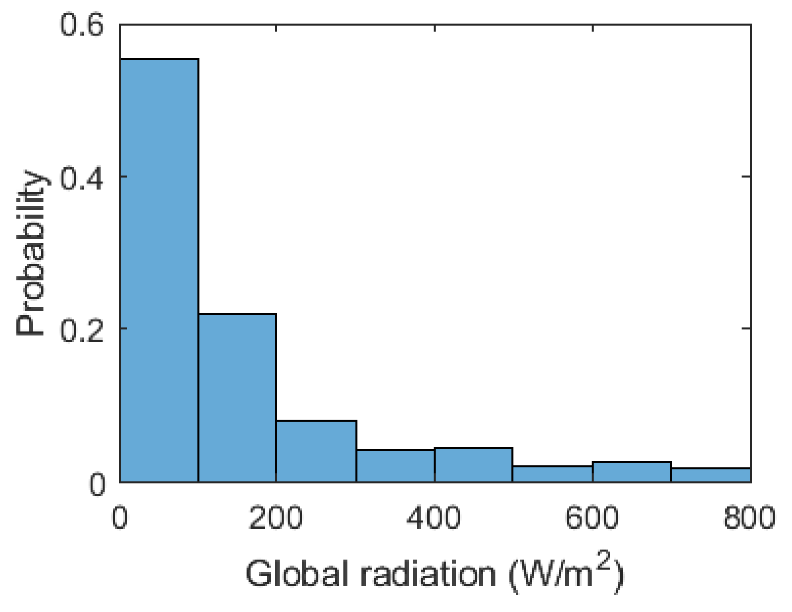
Figure A3.
Histogram of the global radiation for all samples with background radiation. The average value varies depending on the class: 343 W/ (Clear), 104 W/ (Rain), 86 W/ (Fog), 13 W/ (Snow).
Figure A3.
Histogram of the global radiation for all samples with background radiation. The average value varies depending on the class: 343 W/ (Clear), 104 W/ (Rain), 86 W/ (Fog), 13 W/ (Snow).
References
- Wojtanowski, J.; Zygmunt, M.; Kaszczuk, M.; Mierczyk, A.Z.; Muzal, M. Comparison of 905 nm and 1550 nm semiconductor laser rangefinders’ performance deterioration due to adverse environmental conditions. Opto-Electronics Rev. 2014, 22, 183–190. [Google Scholar] [CrossRef]
- Filgueira, A.; González-Jorge, H.; Lagüela, S.; Díaz-Vilariño, L.; Arias, P. Quantifying the influence of rain in LiDAR performance. Meas. 2017, 95, 143–148. [Google Scholar] [CrossRef]
- Rasshofer, R.H.; Spies, M.; Spies, H. Influences of weather phenomena on automotive laser radar systems. Adv. Radio Sci. 2011, 9, 49–60. [Google Scholar] [CrossRef]
- Schöner, H.P. The role of simulation in development and testing of autonomous vehicles. In Proceedings of the Driving Simulation Conference, Stuttgart, Germany, 7 September 2017. [Google Scholar]
- Wood, M.; Knobel, C.; Garbacik, N.; Wittmann, D.; Liu, S.; Syguda, S.; Wiltschko, T.; Weast, J.; Dornieden, B. Safety first for automated driving. Available online: https://newsroom.intel.com/wp-content/uploads/sites/11/2019/07/Intel-Safety-First-for-Automated-Driving.pdf (accessed on 5 July 2019).
- Reif, K. Fahrstabilisierungssysteme und Fahrerassistenzsysteme, 1st ed.; Wiesbaden: Vieweg+ Teubner: Wiesbaden, Germany, 2010. [Google Scholar]
- Shimano, M.; Okawa, H.; Asano, Y.; Bise, R.; Nishino, K.; Sato, I. Wetness and Color from a Single Multispectral Image. In Proceedings of the 2017 IEEE Conference on Computer Vision and Pattern Recognition (CVPR), Honolulu, HI, USA, 22–27 July 2017; pp. 321–329. [Google Scholar]
- McKeen, L.W. The Effect of UV Light and Weather on Plastics and Elastomers; William Andrew: Norwich, NY, USA, 2013. [Google Scholar]
- Rivero, J.R.V.; Tahiraj, I.; Schubert, O.; Glassl, C.; Buschardt, B.; Berk, M.; Chen, J. Characterization and simulation of the effect of road dirt on the performance of a laser scanner. In Proceedings of the 2017 IEEE 20th International Conference on Intelligent Transportation Systems (ITSC), Yokohama, Japan, 16–19 October 2017; pp. 1–6. [Google Scholar] [CrossRef]
- Gaudio, P.; Gelfusa, M.; Malizia, A.; Parracino, S.; Richetta, M.; De Leo, L.; Perrimezzi, C.; Bellecci, C. Detection and monitoring of pollutant sources with Lidar/Dial techniques. J. Physics: Conf. Ser. 2015, 658. [Google Scholar] [CrossRef]
- Ryde, J.; Hillier, N. Performance of laser and radar ranging devices in adverse environmental conditions. J. Field Robot. 2009, 26, 712–727. [Google Scholar] [CrossRef]
- Guo, J.; Zhang, H.; Zhang, X.-J. Propagating Characteristics of Pulsed Laser in Rain. Int. J. Antennas Propag. 2015, 2015, 1–7. [Google Scholar] [CrossRef]
- Dura, M. Modeling the effect of precipitation on automotive LIDAR detection capability. Master’s Thesis, Technical University of Munich, Munich, Germany, 2017. [Google Scholar]
- Dannheim, C.; Icking, C.; Mader, M.; Sallis, P. Weather Detection in Vehicles by Means of Camera and LIDAR Systems. In Proceedings of the Sixth International Conference on Computational Intelligence, Communication Systems and Networks, Tetova, Macedonia, 3–5 June 2014; pp. 186–191. [Google Scholar]
- Charron, N.; Phillips, S.; Waslander, S.L. De-noising of Lidar Point Clouds Corrupted by Snowfall. In Proceedings of the15th Conference on Computer and Robot Vision (CRV), Toronto, ON, Canada, 9–11 May 2018; pp. 254–261. [Google Scholar]
- Kashani, A.G.; Olsen, M.J.; Parrish, C.E.; Wilson, N. A Review of LIDAR Radiometric Processing: From Ad Hoc Intensity Correction to Rigorous Radiometric Calibration. Sensors 2015, 15, 28099–28128. [Google Scholar] [CrossRef] [PubMed]
- Bartell, F.O.; Dereniak, E.L.; Wolfe, W.L. The Theory and Measurement of Bidirectional Reflectance Distribution Function (BRDF) and Bidirectional Transmittance Distribution Function (BTDF). In Proceedings of the Huntsville Technical Symposium, Radiation Scattering in Optical Systems, Huntsville, AL, USA, 3 March 1981; pp. 154–160. [Google Scholar]
- He, W.; Sima, B.; Chen, Y.; Dai, H.; Chen, Q.; Gu, G. A correction method for range walk error in photon counting 3D imaging LIDAR. Opt. Commun. 2013, 308, 211–217. [Google Scholar] [CrossRef]
- Holder, M.; Rosenberger, P.; Bert, F.; Winner, H. Data-driven Derivation of Requirements for a Lidar Sensor Model. In Proceedings of the Graz Symposium Virtual Vehicle, Graz, Austria, 15–16 May 2018. [Google Scholar]
- Wallace, J.M.; Hobbs, P.V. Atmospheric science: An introductory survey, 2nd ed.; Elsevier: Amsterdam, The Netherlands, 2006. [Google Scholar]
- Kim, I.I.; McArthur, B.; Korevaar, E.J. Comparison of laser beam propagation at 785 nm and 1550 nm in fog and haze for optical wireless communications. In Proceedings of the Information Technologies 2000, Boston, MA, USA, 6 February 2001; pp. 26–37. [Google Scholar]
- Thakur, R. Scanning LIDAR in Advanced Driver Assistance Systems and Beyond: Building a road map for next-generation LIDAR technology. IEEE Consum. Electron. Mag. 2016, 5, 48–54. [Google Scholar] [CrossRef]
- Kidono, K.; Miyasaka, T.; Watanabe, A.; Naito, T.; Miura, J. Pedestrian recognition using high-definition LIDAR. In Proceedings of the 2011 IEEE Intelligent Vehicles Symposium (IV), Baden-Baden, Germany, 5–9 June 2011; pp. 405–410. [Google Scholar]
- Carn, S.A. Scattering: Fundamentals of Remote Sensing. Available online: http://pages.mtu.edu/~scarn/teaching/GE4250/scattering_lecture.pdf (accessed on 26 April 2018).
- Liou, K.N.; Yang, P. Light scattering by ice crystals: Fundamentals and applications; Cambridge University Press: Cambridge, UK, 2016. [Google Scholar]
- Moosmüller, H.; Sorensen, C. Small and large particle limits of single scattering albedo for homogeneous, spherical particles. J. Quant. Spectrosc. Radiat. Transf. 2018, 204, 250–255. [Google Scholar] [CrossRef]
- Awan, M.S.; Horwath, L.C.; Muhammad, S.S.; Leitgeb, E.; Nadeem, F.; Khan, M.S. Characterization of Fog and Snow Attenuations for Free-Space Optical Propagation. J. Commun. 2009, 4, 533–545. [Google Scholar] [CrossRef]
- Mohan, M.; Payra, S. Aerosol Number Concentrations and Visibility during Dense Fog over a Subtropical Urban Site. J. Nanomater. 2014, 2014, 1–6. [Google Scholar] [CrossRef]
- Tokay, A.; Bringi, V.; Huang, G.; Schoenhuber, M.; Basho, P.; Wolff, D.; Hudak, D.; Skofronick-Jackson, G.; Petersen, W. Snowflake Size Distribution Measurements in South. Central Ontario, Canada. Available online: https://pmm.nasa.gov/sites/default/files/document_files/parsivel_Tokay_c3vp_agu.pdf (accessed on 26 April 2018).
- Ditze, M.; Golatowski, F.; Laum, N.; Várhelyi, A.; Gustafsson, S.; Geramani, K. A survey on intelligen vehicle safety systems for adverse weather conditions. In Proceedings of the FISITA World Automotive Congress, Budapest, Hungary, 30 May–4 June 2010; pp. 1491–1498. [Google Scholar]
- Andersson, M.; Bruzelius, F.; Casselgren, J.; Hjort, M.; Löfving, S.; Olsson, G.; Rönnber, J.; Sjödahl, M.; Solyom, S.; Svendenius, J.; et al. Road Friction Eestimation, Part II: IVSS Project Report. Available online: http://fudinfo.trafikverket.se/fudinfoexternwebb/Publikationer/Publikationer_001101_001200/Publikation_001109/IVSS_RFEII_Slutrapport.pdf (accessed on 10 November 2010).
- Heinzler, R.; Schindler, P.; Seekircher, J.; Ritter, W.; Stork, W. Weather Influence and Classification with Automotive Lidar Sensors. In Proceedings of the 2019 IEEE Intelligent Vehicles Symposium (IV), Paris, France, 9–12 June 2019; p. 7. [Google Scholar]
- Dannheim, C.; Mader, M.; Loewenau, J.; Icking, C.; Massow, K. A novel approach for the enhancement of cooperative ACC by deriving real time weather information. In Proceedings of the 16th International IEEE Conference on Intelligent Transportation Systems (ITSC 2013), Hague, The Netherlands, 6–9 October 2013; pp. 2207–2211. [Google Scholar]
- Groß, S.; Esselborn, M.; Weinzierl, B.; Wirth, M.; Fix, A.; Petzold, A. Aerosol classification by airborne high spectral resolution lidar observations. Atmos. Chem. Phys. Discuss. 2013, 13, 2487–2505. [Google Scholar] [CrossRef]
- Papagiannopoulos, N.; Mona, L.; Amiridis, V.; Binietoglou, I.; D’Amico, G.; Guma-Claramunt, P.; Schwarz, A.; Alados-Arboledas, L.; Amodeo, A.; Apituley, A.; et al. An automatic aerosol classification for earlinet: Application and results. EPJ Web Conf. 2018, 176. [Google Scholar] [CrossRef][Green Version]
- Koskinen, S.; Peussa, P. Friction: Final Report. Available online: https://trimis.ec.europa.eu/sites/default/files/project/documents/20130411_151442_58182_FRICTION_FinalReport_D13.pdf (accessed on 26 June 2009).
- Bijelic, M.; Gruber, T.; Ritter, W. A benchmark for lidar sensors in fog: Is detection breaking down? In Proceedings of the 2018 IEEE Intelligent Vehicles Symposium (IV), Changshu, China, 26–30 June 2018. [Google Scholar]
- Shamsudin, A.U.; Ohno, K.; Westfechtel, T.; Takahiro, S.; Okada, Y.; Tadokoro, S. Fog removal using laser beam penetration, laser intensity, and geometrical features for 3D measurements in fog-filled room. Adv. Robot. 2016, 30, 1–15. [Google Scholar] [CrossRef]
- James, J.K.; Puhlfürst, G.; Golyanik, V.; Stricker, D. Classification of LIDAR Sensor Contaminations with Deep Neural Networks. In Proceedings of the Computer Science in Cars Symposium (CSCS), Munich, Germany, 13–14 September 2018; p. 8. [Google Scholar]
- Mobley, C.D. Light and Water: Radiative Transfer in Natural Waters; Academic Press: New York, NY, USA, 1994. [Google Scholar]
- Bayerisches Landesamt für Umwelt, Gewässerkundlicher Dienst Bayern. Available online: https://www.gkd.bayern.de/de/meteo/niederschlag/kelheim/hepberg-200106/download (accessed on 30 July 2020).
- Markvart, T.; McEvoy, A.; Castaner, L. Practical Handbook of Photovoltaics: Fundamentals and Applications; Elsevier: Amsterdam, The Netherlands, 2003. [Google Scholar]
- Pavement Albedo. Available online: https://web.archive.org/web/20070829153207/http://eetd.lbl.gov/HeatIsland/Pavements/Albedo/ (accessed on 18 October 2019).
- Sasaki, Y. The truth of the F-measure. Available online: https://www.researchgate.net/publication/268185911_The_truth_of_the_F-measure/citation/download (accessed on 18 October 2019).
- Fink, C.; Russ Moulton Jr, J.; Bybee, D.; George, K. GPU Raytracing for real-time sensor-band phenomenology modeling. In Proceedings of the IMAGE Society, Dayton, OH, USA, 22–23 June 2012. [Google Scholar]
- Kavak, Ç. GPU Based Infrared Signature Modeling and Scene Simulation. Master’s Thesis, Middle East Technical University, Ankara, Turkey, 2014. [Google Scholar]
- Jalalmaab, M.; Pirani, M.; Fidan, B.; Jeon, S. Cooperative Estimation of Road Condition Based on Dynamic Consensus and Vehicular Communication. IEEE Trans. Intell. Veh. 2018, 4, 90–100. [Google Scholar] [CrossRef]
- Cheng, G.; Wang, Z.; Zheng, J.Y. Modeling Weather and Illuminations in Driving Views Based on Big-Video Mining. IEEE Trans. Intell. Veh. 2018, 3, 522–533. [Google Scholar] [CrossRef]
- Brunker, A.; Wohlgemuth, T.; Frey, M.; Gauterin, F.; Alexander, B. Odometry 2.0: A Slip-Adaptive EIF-Based Four-Wheel-Odometry Model for Parking. IEEE Trans. Intell. Veh. 2018, 4, 114–126. [Google Scholar] [CrossRef]
Figure 1.
Illustration of the parameters used in the bathymetric LIDAR equation. Although the used LIDAR is not a bathymetric LIDAR the equation is used to show the dependencies present when the amount of water on top of a certain surface is high. These dependencies are used for the analysis of the street region when covered by water in
Section 4.
Figure 2.
Relation between TOF and intensity for a received pulse. If the noise level increases (blue) no detection is registered. The sent pulse (idealized) is shown in red and the received signal in black.
Figure 2.
Relation between TOF and intensity for a received pulse. If the noise level increases (blue) no detection is registered. The sent pulse (idealized) is shown in red and the received signal in black.
Figure 3.
Depiction of the measurement setup. Left: schematic front view of the LIDAR sensor position and its effective field of view (A: atmosphere region, B: street region), the used axis corresponds to the LIDAR coordinate system. Middle: example of the obtained point cloud (birds eye view). Right: Picture from top of the building. The field of view of the sensor is illustrated by the red triangle.
Figure 4.
Parameters used to characterize the distributions in the atmosphere and street region.
Figure 4.
Parameters used to characterize the distributions in the atmosphere and street region.
Figure 5.
Distribution of the detections for each weather class (1900 frames each) in the atmosphere region (0-5 m) (w/o) without and (w) with background radiation. With : standard deviation of the detection distance in x-direction in cm.
Figure 5.
Distribution of the detections for each weather class (1900 frames each) in the atmosphere region (0-5 m) (w/o) without and (w) with background radiation. With : standard deviation of the detection distance in x-direction in cm.
Figure 6.
Distribution of the detections for each weather class (1900 frames each) in the street region: (w/o) without and (w) with background radiation. With : standard deviation of the detection distance in x-direction in cm.
Figure 6.
Distribution of the detections for each weather class (1900 frames each) in the street region: (w/o) without and (w) with background radiation. With : standard deviation of the detection distance in x-direction in cm.
Table 1.
Typical atmospheric scattering particles with their average size parameter for a wavelength from 905 nm and concentration [
21,
24,
27,
28,
29].
Table 1.
Typical atmospheric scattering particles with their average size parameter for a wavelength from 905 nm and concentration [
21,
24,
27,
28,
29].
| Type | Radius (µm) | Size Parameter | Concentration |
|---|
| Air molecules | 0.0001 | 0.0007 | <3 × |
| Haze, smoke, dust | 0.01–1 | 0.07 | –5 × |
| Fog | 1–20 | 7–139 | –5 × |
| Rain | 100–10000 | 694–69427 | 10– |
| Snow | 1000–5000 | 6943–34714 | – |
| Hail | 5000–50000 | 34714–347137 | –1 |
Table 2.
Influence of background radiation on the total number of echoes and EPW for 1900 frames during the day and 1900 during the night including both regions during clear weather. The results show mean value ± standard deviation.
Table 2.
Influence of background radiation on the total number of echoes and EPW for 1900 frames during the day and 1900 during the night including both regions during clear weather. The results show mean value ± standard deviation.
| | | |
|---|
| 257 ± 19 | 66 ± 67 | 1.21 ± 0.39 |
| 190 ± 110 | 20 ± 25 | 0.93 ± 0.27 |
Table 3.
Most important parameters for the atmosphere region (0–5 m)*. (w/o) Without background radiation, (w) with background radiation. With : total number of detections in the region, : number of detections in the maximum, : standard deviation of the detection distance, : number of first echo detections and : echo-pulse width. The results show mean value ± standard deviation.
| | Clear | Fog | Rain | Snow |
|---|
| | w | w/o | w | w/o | w | w/o | w | w/o |
|---|
| 86 ± 34 | 244 ± 16 | 114 ± 14 | 313 ± 55 | 238 ± 161 | 661 ± 113 | 137 ± 13 | 344 ± 57 |
| 55 ± 18 | 113 ± 19 | 74 ± 14 | 124 ± 34 | 159 ± 124 | 287 ± 60 | 79 ± 14 | 126 ± 21 |
| [cm] | 5 ± 11 | 10 ± 8 | 3 ± 2 | 7 ± 5 | 3 ± 3 | 15 ± 8 | 57 ± 22 | 84 ± 23 |
| 86 ± 34 | 244 ± 16 | 114 ± 14 | 313 ± 55 | 238 ± 161 | 659 ± 112 | 135 ± 12 | 324 ± 46 |
| [m] | 0.75 ± 0.29 | 0.95 ± 0.35 | 0.82 ± 0.29 | 0.94 ± 0.34 | 0.86 ± 0.30 | 1.00 ± 0.35 | 0.86 ± 0.32 | 1.02 ± 0.38 |
Table 4.
Most important parameters for the street region (33–37 m). (w/o) Without background radiation, (w) with background radiation. With : number of detections in the maximum, : mean detection distance, : standard deviation of the detection distance, : number of second echo detections and : echo-pulse width. The results show mean value ± standard deviation.
| | Clear | Fog | Rain | Snow |
|---|
| | w | w/o | w | w/o | w | w/o | w | w/o |
|---|
| 77 ± 39 | 45 ± 37 | 88 ± 30 | 72 ± 26 | 97 ± 39 | 125 ± 33 | 89 ± 30 | 132 ± 33 |
| [cm]* | 74 ± 15 | 96 ± 27 | 73 ± 02 | 74 ± 03 | 69 ± 03 | 71 ± 03 | 70 ± 05 | 60 ± 03 |
| [cm] | 27 ± 22 | 68 ± 30 | 17 ± 5 | 24 ± 5 | 21 ± 5 | 31 ± 7 | 22 ± 8 | 37 ± 9 |
| 40 ± 21 | 131 ± 20 | 37 ± 11 | 128 ± 21 | 52 ± 19 | 300 ± 52 | 51 ± 9 | 193 ± 32 |
| EPW [m] | 1.10 ± 0.24 | 1.48 ± 0.23 | 1.02 ± 0.25 | 1.09 ± 0.30 | 1.01 ± 0.26 | 1.22 ± 0.33 | 1.03 ± 0.26 | 1.63 ± 0.30 |
Table 5.
Confusion matrix for the atmosphere region without background radiation (left, 6130 samples per class) and with background radiation (right, 1930 samples per class) (classifier: Weighted KNN).
Table 5.
Confusion matrix for the atmosphere region without background radiation (left, 6130 samples per class) and with background radiation (right, 1930 samples per class) (classifier: Weighted KNN).
| | | Predicted Class |
|---|
| | | Without Background Radiation | With Background Radiation |
|---|
| | Clear | Rain | Fog | Snow | Clear | Rain | Fog | Snow |
|---|
| Actual Class | Clear | 5284 | 1 | 844 | 1 | 1670 | 32 | 188 | 40 |
| Rain | 3 | 6055 | 32 | 40 | 0 | 1877 | 43 | 10 |
| Fog | 980 | 16 | 5132 | 2 | 58 | 80 | 1785 | 7 |
| Snow | 2 | 19 | 1 | 6108 | 0 | 50 | 42 | 1838 |
| | F-Score | 84.97 | 99.04 | 84.36 | 99.42 | 91.42 | 94.74 | 89.78 | 96.23 |
Table 6.
Confusion matrix for the street region without background radiation (left, 6130 samples per class) and with background radiation (right, 1930 samples per class) (classifier: Weighted KNN).
Table 6.
Confusion matrix for the street region without background radiation (left, 6130 samples per class) and with background radiation (right, 1930 samples per class) (classifier: Weighted KNN).
| | | Predicted Class |
|---|
| | | Without Background Radiation | With Background Radiation |
|---|
| | Clear | Rain | Fog | Snow | Clear | Rain | Fog | Snow |
|---|
| Actual Class | Clear | 5462 | 0 | 667 | 1 | 1761 | 32 | 112 | 25 |
| Rain | 0 | 6078 | 52 | 0 | 5 | 1912 | 1 | 12 |
| Fog | 315 | 6 | 5809 | 0 | 13 | 0 | 1900 | 17 |
| Snow | 11 | 0 | 3 | 6116 | 0 | 0 | 13 | 1917 |
| | F-Score | 91.62 | 99.45 | 91.67 | 99.89 | 95.04 | 98.71 | 96.11 | 98.31 |
Table 7.
Results of the feature ablation analysis for the atmosphere region using the F1-Score as evaluation parameter. In comparison with the score using all features, the features are marked with ✓ when the F1-Score for two or more classes decreases more than 0.4 (marked in grey), with ✕ when increases more than 0.4 (marked in blue) and with - in other cases (All- is marked as neutral because the F1-Score of Clear increases).
| Feature | Atmosphere w/o BR (F1-Score) | Atmosphere w BR (F1-Score) | Evaluation |
|---|
| Clear | Rain | Fog | Snow | Clear | Rain | Fog | Snow |
|---|
| All | 84.97 | 99.04 | 84.36 | 99.42 | 91.42 | 94.74 | 89.78 | 96.23 | |
| All- | 85.11 | 98.94 | 84.48 | 99.36 | 91.10 | 94.23 | 89.15 | 96.05 | ✓ |
| All- | 84.83 | 99.11 | 84.34 | 99.41 | 91.54 | 94.76 | 89.65 | 96.02 | - |
| All- | 84.50 | 99.04 | 83.85 | 99.40 | 91.04 | 94.65 | 89.16 | 96.10 | ✓ |
| All- | 84.94 | 99.11 | 84.24 | 99.48 | 91.60 | 94.54 | 89.74 | 96.11 | - |
| All- | 84.71 | 99.02 | 84.01 | 99.31 | 91.40 | 94.38 | 89.12 | 95.17 | ✓ |
| All- | 84.76 | 99.09 | 84.18 | 99.47 | 91.36 | 94.66 | 89.49 | 96.16 | - |
| All- | 85.62 | 99.12 | 85.20 | 99.38 | 91.25 | 94.67 | 89.64 | 96.13 | ✕ |
| All- | 84.43 | 99.04 | 83.84 | 99.42 | 91.20 | 94.86 | 89.26 | 96.18 | ✓ |
| All- | 85.21 | 99.09 | 84.50 | 99.49 | 91.37 | 94.43 | 89.55 | 96.02 | - |
| All- | 85.25 | 99.11 | 84.63 | 99.44 | 91.50 | 94.59 | 89.63 | 96.21 | - |
| All- | 82.01 | 98.09 | 80.71 | 98.79 | 91.55 | 92.51 | 88.22 | 95.48 | ✓ |
| All- | 84.86 | 98.92 | 84.21 | 99.47 | 91.93 | 93.59 | 88.55 | 96.42 | - |
Table 8.
Results of the feature ablation analysis for the atmosphere region using the F1-Score as evaluation parameter. In comparison with the score using all features the features are marked with ✓ when the F1-Score for two or more classes decreases more than 0.4 (marked in gray), with ✕ when increases more than 0.4 (marked in blue) and with - in other cases.
| Feature | Street w/o BR (F1-Score) | Street w BR (F1-Score) | Evaluation |
|---|
| Clear | Rain | Fog | Snow | Clear | Rain | Fog | Snow |
|---|
| All | 91.62 | 99.45 | 91.67 | 99.89 | 95.04 | 98.71 | 96.11 | 98.31 | |
| All- | 91.19 | 99.51 | 91.42 | 99.81 | 95.18 | 98.71 | 96.23 | 98.15 | ✓ |
| All- | 91.62 | 99.37 | 91.66 | 99.85 | 94.94 | 98.79 | 95.89 | 98.18 | - |
| All- | 91.63 | 99.44 | 91.67 | 99.90 | 94.89 | 98.76 | 95.93 | 98.23 | - |
| All- | 91.58 | 99.23 | 91.42 | 99.90 | 94.09 | 98.63 | 94.80 | 98.10 | ✓ |
| All- | 91.67 | 99.50 | 91.77 | 99.89 | 94.70 | 98.50 | 95.94 | 97.87 | ✓ |
| All- | 91.44 | 99.46 | 91.58 | 99.82 | 94.90 | 98.66 | 96.04 | 98.31 | - |
| All- | 91.57 | 99.62 | 91.75 | 99.89 | 95.98 | 98.91 | 96.67 | 98.39 | ✕ |
| All- | 91.35 | 99.37 | 91.32 | 99.89 | 94.76 | 98.61 | 95.91 | 98.05 | - |
| All- | 91.32 | 99.42 | 91.33 | 99.91 | 93.76 | 97.86 | 95.31 | 96.51 | ✓ |
| All- | 91.55 | 99.45 | 91.68 | 99.77 | 96.15 | 98.87 | 96.95 | 99.07 | - |
| All- | 91.07 | 99.27 | 90.99 | 99.86 | 94.00 | 97.91 | 95.49 | 97.67 | ✓ |
| All- | 92.05 | 99.55 | 92.08 | 99.95 | 95.79 | 99.07 | 96.61 | 98.59 | ✕ |
Table 9.
F1-Score per class for the atmosphere region when using only the parameters: .
Table 9.
F1-Score per class for the atmosphere region when using only the parameters: .
| Atmosphere w/o BR (F1-Score) | Atmosphere w BR (F1-Score) |
|---|
| Clear | Rain | Fog | Snow | Clear | Rain | Fog | Snow |
|---|
| 85.30 | 98.82 | 84.82 | 99.27 | 92.54 | 93.27 | 89.01 | 96.86 |
Table 10.
F1-Score per class for the street region when using the parameters: , , , .
Table 10.
F1-Score per class for the street region when using the parameters: , , , .
| Street w/o BR (F1-Score) | Street w BR (F1-Score) |
|---|
| Clear | Rain | Fog | Snow | Clear | Rain | Fog | Snow |
|---|
| 91.29 | 99.43 | 91.42 | 99.76 | 96.67 | 99.09 | 96.81 | 98.86 |
© 2020 by the authors. Licensee MDPI, Basel, Switzerland. This article is an open access article distributed under the terms and conditions of the Creative Commons Attribution (CC BY) license (http://creativecommons.org/licenses/by/4.0/).

 ,
, 


