Fully Automated Segmentation of Bladder Sac and Measurement of Detrusor Wall Thickness from Transabdominal Ultrasound Images

 ,
,  , and
, and
Abstract

1. Introduction
2. Materials and Methods
2.1. Data Acquisition
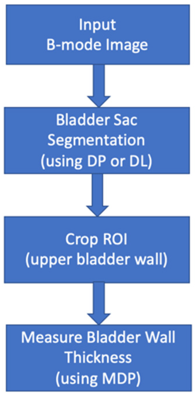
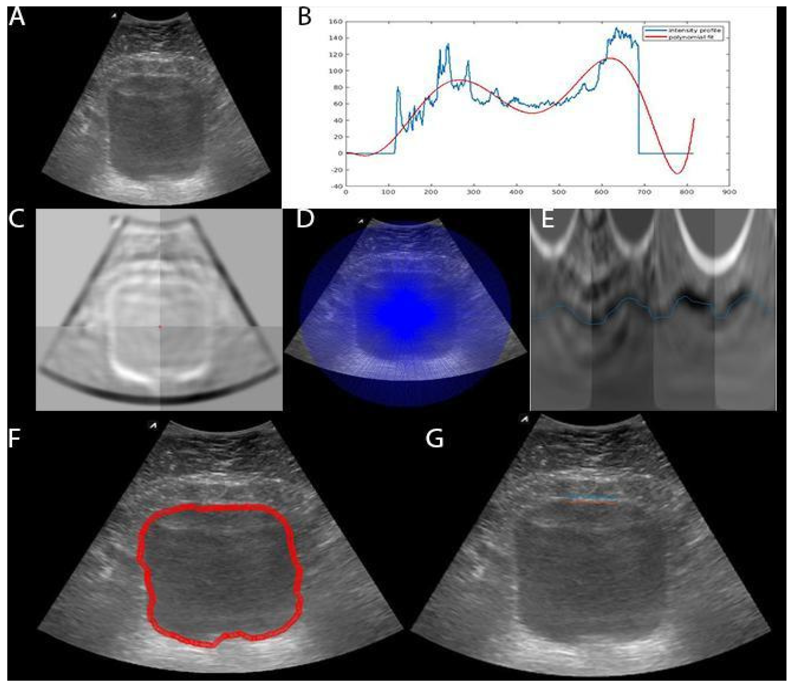
2.2. Bladder Segmentation
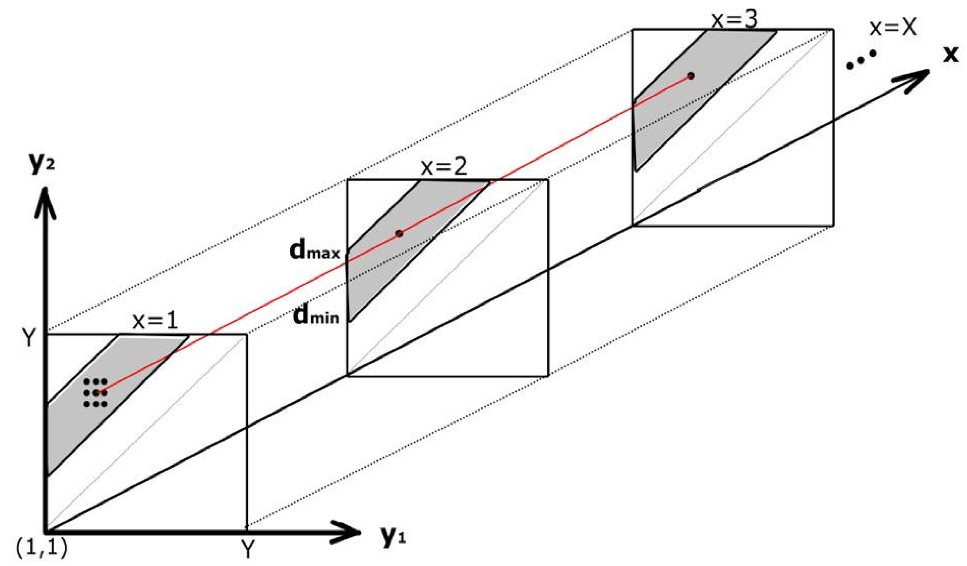
2.2.1. Dynamic Programming (DP)
2.2.2. Deep Learning (DL)
2.3. Bladder Wall Thickness Measurement
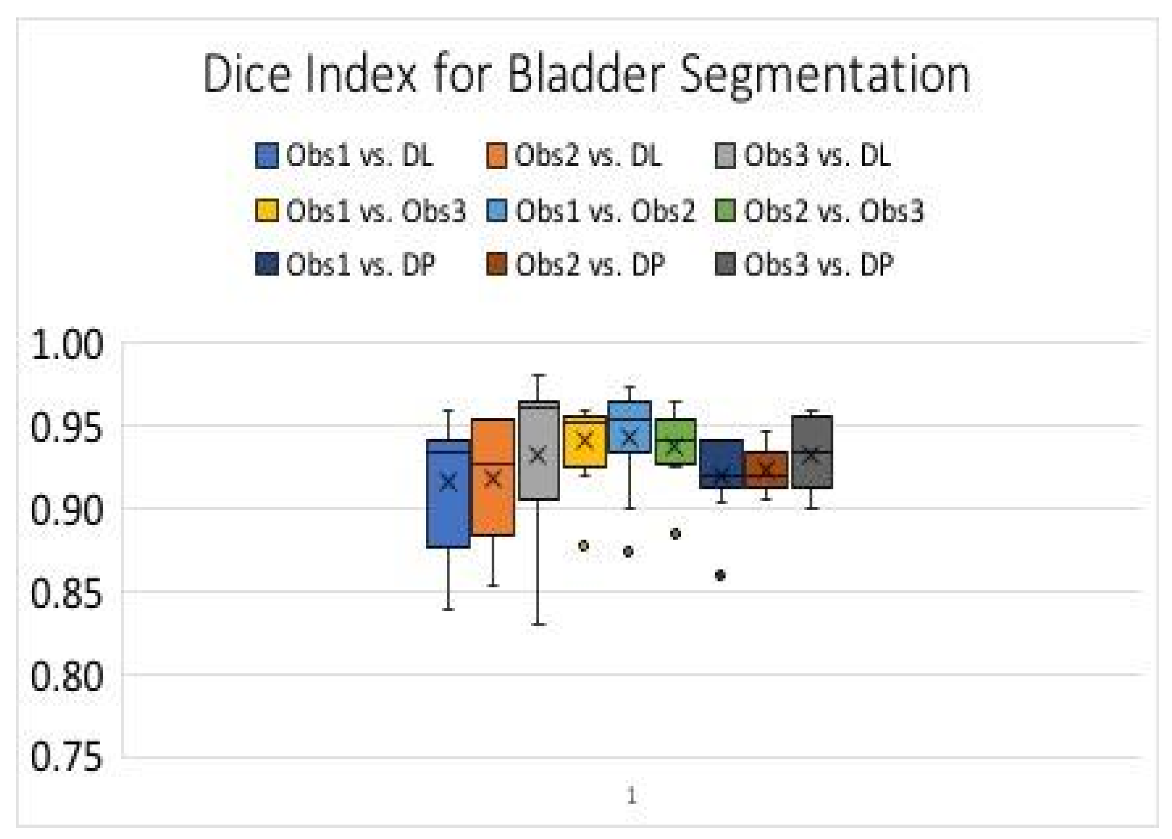
2.4. Evaluations
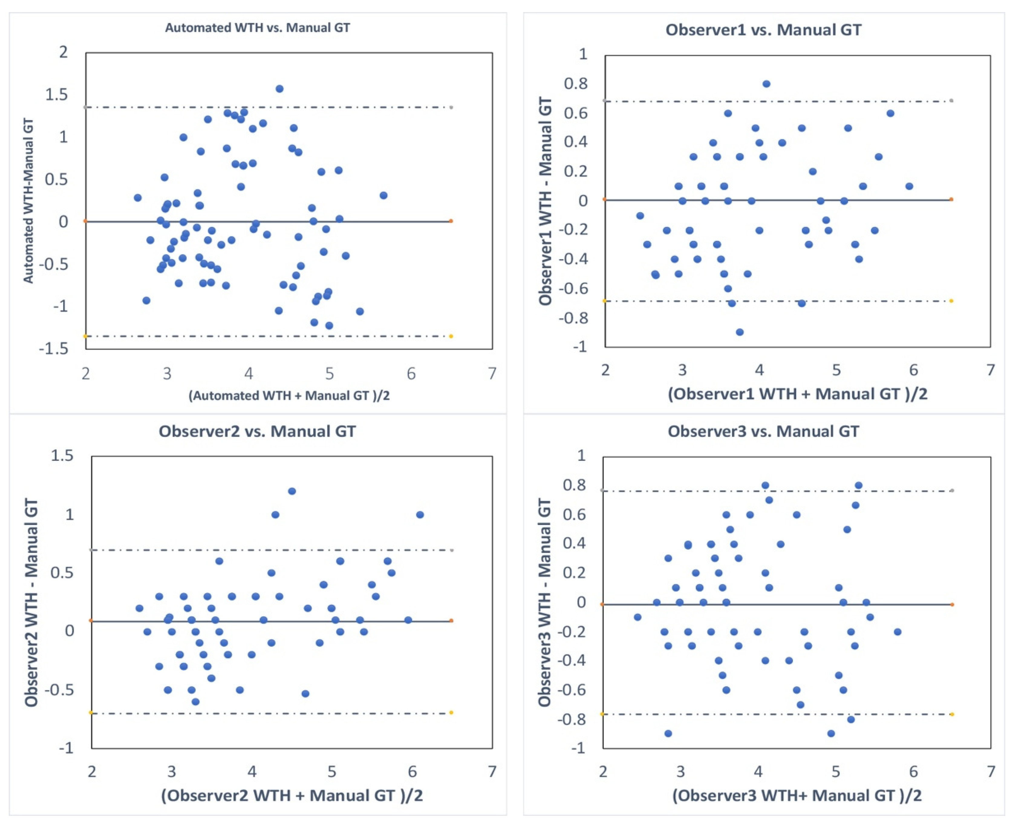
3. Results
4. Discussion
5. Conclusions
Author Contributions
Funding
Acknowledgments
Conflicts of Interest
References
- Manieri, C.; Carter, S.S.; Romano, G.; Trucchi, A.; Valenti, M.; Tubaro, A. The diagnosis of bladder outlet obstruction in men by ultrasound measurement of bladder wall thickness. J. Urol. 1998, 159, 761–765. [Google Scholar] [CrossRef]
- Hakenberg, O.W.; Linne, C.; Manseck, A.; Wirth, M.P. Bladder Wall Thickness in Normal Adults and Men with Mild Lower Urinary Tract Symptoms and Benign Prostatic Enlargement. Neurourol. Urodyn. 2000, 19, 585–593. [Google Scholar] [CrossRef]
- Oelke, M.; Höfner, K.; Wiese, B.; Grünewald, V.; Jonas, U. Increase in Detrusor Wall Thickness Indicates Bladder Outlet Obstruction (BOO) in Men. World J. Urol. 2002, 19, 443–452. [Google Scholar] [CrossRef] [PubMed]
- Kessler, T.M.; Gerber, R.; Burkhard, F.C.; Studer, U.E.; Danuser, H. Ultrasound Assessment of Detrusor Thickness in Men—Can it Predict Bladder Outlet Obstruction and Replace Pressure Flow Study? J. Urol. 2006, 175, 2170–2173. [Google Scholar] [CrossRef]
- Oelke, M.; Höfner, K.; Jonas, U.; de la Rosette, J.J.; Ubbink, D.T.; Wijkstra, H. Diagnostic Accuracy of Noninvasive Tests to Evaluate Bladder Outlet Obstruction in Men: Detrusor Wall Thickness, Uroflowmetry, Postvoid Residual Urine, and Prostate Volume. Eur. Urol. 2007, 52, 827–834. [Google Scholar] [CrossRef] [PubMed]
- Hill, P. Can Ultrasound Replace Ambulatory Urodynamics when Investigating Women with Irritative Urinary Symptoms? BJOG 2002, 109, 1422. [Google Scholar] [CrossRef]
- Kuhn, A.; Bank, S.; Robinson, D.; Klimek, M.; Kuhn, P.; Raio, L. How should Bladder Wall Thickness be Measured? A Comparison of Vaginal, Perineal and Abdominal Ultrasound. Neurourol. Urodyn. 2010, 29, 1393–1396. [Google Scholar] [CrossRef]
- Khullar, V.; Cardozo, L.D.; Salvatore, S.; Hill, S. Ultrasound: A Noninvasive Screening Test for Detrusor Instability. Br. J. Obstet. Gynaecol. 1996, 103, 904–908. [Google Scholar] [CrossRef]
- Khullar, V.; Salvatore, S.; Cardozo, L.; Bourne, T.H.; Abbott, D.; Kelleher, C. A Novel Technique for Measuring Bladder Wall Thickness in Women using Transvaginal Ultrasound. Ultrasound Obstet. Gynecol. 1994, 4, 220–223. [Google Scholar] [CrossRef]
- Cvitković-Kuzmić, A.; Brkljacić, B.; Ivanković, D.; Grga, A. Ultrasound Assessment of Detrusor Muscle Thickness in Children with Non–Neuropathic Bladder/Sphincter Dysfunction. Eur. Urol. 2002, 41, 214–218. [Google Scholar] [CrossRef]
- Kaefer, M.; Barnewolt, C.; Retik, A.B.; Peters, C.A. The Sonographic Diagnosis of Infravesical Obstruction in Children: Evaluation of Bladder Wall Thickness Indexed to Bladder Filling. J. Urol. 1997, 157, 989–991. [Google Scholar] [CrossRef]
- Adibi, A.; Kazemian, A.; Toghiani, A. Normal Bladder Wall Thickness Measurement in Healthy Iranian Children, A Cross–Sectional Study. Adv. Biomed. Res. 2014, 3, 1–10. [Google Scholar] [CrossRef] [PubMed]
- Yeung, C.-K.; Sreedhar, B.; Leung, Y.-F.V.; Sit, K.-Y.F. Correlation Between Ultrasonographic Bladder Measurements and Urodynamic Findings in Children with Recurrent Urinary Tract Infection. BJU Int. 2007, 99, 651–655. [Google Scholar] [CrossRef] [PubMed]
- Bayat, M.; Kumar, V.; Denis, M.; Webb, J.; Gregory, A.; Mehrmohammadi, M.; Cheong, M.; Husmann, D.; Mynderse, L.; Alizad, A.; et al. Correlation of Ultrasound Bladder Vibrometry Assessment of Bladder Compliance with Urodynamic Study Results. PloS ONE 2017, 12, e0179598. [Google Scholar] [CrossRef]
- Nenadic, I.; Mynderse, L.; Husmann, D.; Mehrmohammadi, M.; Bayat, M.; Singh, A.; Denis, M.; Urban, M.; Alizad, A.; Fatemi, M. Noninvasive Evaluation of Bladder Wall Mechanical Properties as a Function of Filling Volume: Potential Application in Bladder Compliance Assessment. PLoS ONE 2016, 11, e0157818. [Google Scholar] [CrossRef]
- Nenadic, I.Z.; Qiang, B.; Urban, M.W.; de Araujo Vasconcelo, L.H.; Nabavizadeh, A.; Alizad, A.; Greenleaf, J.F.; Fatemi, M. Ultrasound Bladder Vibrometry Method for Measuring Viscoelasticity of the Bladder Wall. Phys. Med. Biol. 2013, 58, 2675. [Google Scholar] [CrossRef]
- Oelke, M.; Mamoulakis, C.; Ubbink, D.T.; de la Rosette, J.J.; Wijkstra, H. Manual Versus Automatic Bladder Wall Thickness Measurements: A Method Comparison Study. World J. Urol. 2009, 27, 747–753. [Google Scholar] [CrossRef][Green Version]
- Farag, F.F.; Heesakkers, J.P. Noninvasive techniques in the diagnosis of bladder storage disorders. Neurourol. Urodyn. 2011, 30, 1422–1428. [Google Scholar] [CrossRef]
- Akkus, Z.; Hoogi, A.; Renaud, G.; ten Kate, G.L.; van den Oord, S.C.; Schinkel, A.F.; de Jong, N.; van der Steen, A.F.; Bosch, J.G. Motion compensation method using dynamic programming for quantification of neovascularization in carotid atherosclerotic plaques with contrast enhanced ultrasound (CEUS). In Proceedings of the Medical Imaging 2012: Ultrasonic Imaging, Tomography, and Therapy, San Diego, CA, USA, 5–6 February 2012. [Google Scholar]
- Akkus, Z.; Bayat, M.; Cheong, M.; Viksit, K.; Erickson, B.J.; Alizad, A.; Fatemi, M. Fully Automated and Robust Tracking of Transient Waves in Structured Anatomies Using Dynamic Programming. Ultrasound Med. Biol. 2016, 42, 2504–2512. [Google Scholar] [CrossRef]
- Akkus, Z.; Carvalho, D.D.; van den Oord, S.C.; Schinkel, A.F.; Niessen, W.J.; de Jong, N.; van der Steen, A.F.; Klein, S.; Bosch, J.G. Fully Automated Carotid Plaque Segmentation in Combined Contrast-Enhanced and B-Mode Ultrasound. Ultrasound Med. Biol. 2015, 41, 517–531. [Google Scholar] [CrossRef]
- Bellman, R. Dynamic programming. Science 1966, 153, 34–37. [Google Scholar] [CrossRef] [PubMed]
- Timp, S.; Karssemeijer, N. A New 2D Segmentation Method Based on Dynamic Programming Applied to Computer Aided Detection in Mammography. Med. Phys. 2004, 31, 958–971. [Google Scholar] [CrossRef] [PubMed]
- Hareendranathan, A.R.; Mabee, M.; Punithakumar, K.; Noga, M.; Jaremko, J.L. A Technique for Semiautomatic Segmentation of Echogenic Structures in 3D Ultrasound, Applied to Infant Hip Dysplasia. Int. J. Comput. Assist. Radiol. Surg. 2016, 11, 31–42. [Google Scholar] [CrossRef] [PubMed]
- Ronneberger, O.; Fischer, P.; Brox, T. U-Net: Convolutional networks for biomedical image segmentation. In Proceedings of the 18th International Conference, Munich, Germany, 5–9 October 2015. [Google Scholar]
- Akkus, Z.; Galimzianova, A.; Hoogi, A.; Rubin, D.L.; Erickson, B.J. Deep Learning for Brain MRI Segmentation: State of the Art and Future Directions. J. Digit. Imaging. 2017, 30, 449–459. [Google Scholar] [CrossRef] [PubMed]
- Glorot, X.; Bengio, Y. Understanding the difficulty of training deep feedforward neural networks. In Proceedings of the Thirteenth International Conference on Artificial Intelligence and Statistics, Sardinia, Italy, 13–15 May 2010. [Google Scholar]
- Srivastava, N.; Geoffrey, H.; Krizhevsky, A.; Sutskever, I.; Salakhutdinov, R. Dropout: A Simple Way to Prevent Neural Networks from Overfitting. J. Mach. Learn. Res. 2014, 15, 1929–1958. [Google Scholar]
- Kingma, D.P.; Ba, J. Adam: A Method for Stochastic Optimization. arXiv 2014, arXiv:1412.6980. [Google Scholar]
- Yang, J.-M.; Huang, W.-C. Bladder Wall Thickness on Ultrasonographic Cystourethrography: Affecting Factors and their Implications. J. Ultrasound Med. 2003, 22, 777–782. [Google Scholar] [CrossRef]


| BWT | RMSE (mm) |
|---|---|
| MDP vs. GT | 0.7 ± 0.21 |
| Obs1 vs. Obs2 | 0.55 ± 0.21 |
| Obs1 vs. Obs3 | 0.63 ± 0.27 |
| Obs2 vs. Obs3 | 0.69 ± 0.25 |
© 2020 by the authors. Licensee MDPI, Basel, Switzerland. This article is an open access article distributed under the terms and conditions of the Creative Commons Attribution (CC BY) license (http://creativecommons.org/licenses/by/4.0/).
Share and Cite
Akkus, Z.; Kim, B.H.; Nayak, R.; Gregory, A.; Alizad, A.; Fatemi, M. Fully Automated Segmentation of Bladder Sac and Measurement of Detrusor Wall Thickness from Transabdominal Ultrasound Images. Sensors 2020, 20, 4175. https://doi.org/10.3390/s20154175
Akkus Z, Kim BH, Nayak R, Gregory A, Alizad A, Fatemi M. Fully Automated Segmentation of Bladder Sac and Measurement of Detrusor Wall Thickness from Transabdominal Ultrasound Images. Sensors. 2020; 20(15):4175. https://doi.org/10.3390/s20154175
Chicago/Turabian StyleAkkus, Zeynettin, Bae Hyung Kim, Rohit Nayak, Adriana Gregory, Azra Alizad, and Mostafa Fatemi. 2020. "Fully Automated Segmentation of Bladder Sac and Measurement of Detrusor Wall Thickness from Transabdominal Ultrasound Images" Sensors 20, no. 15: 4175. https://doi.org/10.3390/s20154175
APA StyleAkkus, Z., Kim, B. H., Nayak, R., Gregory, A., Alizad, A., & Fatemi, M. (2020). Fully Automated Segmentation of Bladder Sac and Measurement of Detrusor Wall Thickness from Transabdominal Ultrasound Images. Sensors, 20(15), 4175. https://doi.org/10.3390/s20154175