Wavefront Aberration Sensor Based on a Multichannel Diffractive Optical Element


Abstract
:1. Introduction
2. Theoretical Background
3. Experiments on Detection of Various Wavefront Aberrations Using a Zernike Filter
4. Experiments on the Collimator Fine-Tuning
5. Conclusions
Author Contributions
Funding
Conflicts of Interest
References
- David, F. Buscher Practical Optical Interferometry; Cambridge University Press: Cambridge, UK, 2015. [Google Scholar] [CrossRef]
- Malacara, D. Optical Shop Testing; John Wiley & Sons, Inc.: Hoboken, NJ, USA, 2007; ISBN 978-0-471-48404-2. [Google Scholar]
- Vasil’ev, L.A. Schlieren Methods; Israel Program For Scientific Translations: New York, NY, USA; Jerusalem, Israel; London, UK, 1971. [Google Scholar]
- Hartmann, J. Bemerkungen über den Bau und die Justierung von Spektrographen. Z. Für Instrum. 1900, 20, 47. [Google Scholar]
- Artzner, G. Microlens arrays for Shack-Hartmann wavefront sensors. Opt. Eng. 1992, 31, 1311–1322. [Google Scholar] [CrossRef]
- Platt, B.C.; Shack, R. History and principles of Shack-Hartmann wavefront sensing. J. Refract. Surg. 2001, 17, S573–S577. [Google Scholar] [CrossRef] [PubMed]
- Hongbin, Y.; Guangya, Z.; Siong, C.F.; Feiwen, L.; Shouhua, W.A. Tunable Shack-Hartmann wavefront sensor based on a liquid-filled microlens array. J. Micromech. Microeng. 2008, 18, 105017. [Google Scholar] [CrossRef]
- Minin, I.; Minin, O. Diffractive Optics and Nanophotonics. Resolution Below the Diffraction Limit; Springer International Publishing: Cham, Switzerland, 2015. [Google Scholar] [CrossRef]
- Zernike, F. Beugungstheorie des schneidenver-fahrens und seiner verbesserten form, der phasenkontrastmethode. Physica 1934, 1, 689–704. [Google Scholar] [CrossRef]
- Nijboer, B.R.A. The diffraction theory of optical aberrations: Part I: General discussion of the geometrical aberrations. Physica 1943, 10, 679–692. [Google Scholar] [CrossRef]
- Nijboer, B.R.A. The diffraction theory of optical aberrations: Part II: Diffraction pattern in the presence of small aberrations. Physica 1947, 13, 605–620. [Google Scholar] [CrossRef]
- Nienhuis, K.; Nijboer, B.R.A. The diffraction theory of optical aberrations: Part III: General formulae for small aberrations; experimental verification of the theoretical results. Physica 1949, 14, 590–604. [Google Scholar] [CrossRef]
- Born, M.; Wolf, E. Principles of Optics: Electromagnetic Theory of Propagation, Interference and Diffraction of Light, 7th ed.; Cambridge University Press: Cambridge, UK, 1999. [Google Scholar]
- Roddier, N. Atmospheric wavefront simulation using Zernike polynomials. Opt. Eng. 1990, 29, 1174–1180. [Google Scholar] [CrossRef]
- Neil, M.A.A.; Booth, M.J.; Wilson, T. New modal wave-front sensor: A theoretical analysis. J. Opt. Soc. Am. A 2000, 17, 1098–1107. [Google Scholar] [CrossRef]
- Thibos, L.N.; Applegate, R.A.; Schwiegerling, J.T.; Webb, R. Standards for reporting the optical aberrations of eyes. J. Refract. Surg. 2002, 18, S652–S660. [Google Scholar] [CrossRef] [PubMed]
- Evans, C.J.; Parks, R.E.; Sullivan, P.J.; Taylor, J.S. Visualization of surface figure by the use of Zernike polynomials. Appl. Opt. 1995, 34, 7815–7819. [Google Scholar] [CrossRef] [PubMed]
- Methods for Reporting Optical Aberrations of Eyes, ANSI Z80.28; American National Standards Institute, Inc.: New York, NY, USA, 2004.
- Lombardo, M.; Lombardo, G. Wave aberration of human eyes and new descriptors of image optical quality and visual performance. J. Cataract. Refr. Surg. 2010, 36, 313–331. [Google Scholar] [CrossRef]
- Khorin, P.A.; Khonina, S.N.; Karsakov, A.V.; Branchevskiy, S.L. Analysis of corneal aberration of the human eye. Comput. Opt. 2016, 40, 810–817. [Google Scholar] [CrossRef]
- Martins, A.C.; Vohnsen, B. Measuring ocular aberrations sequentially using a digital micromirror device. Micromachines 2019, 10, 117. [Google Scholar] [CrossRef] [Green Version]
- Soifer, V.A. Methods for Computer Design of Diffractive Optical Elements; John Wiley & Sons, Inc.: New York, NY, USA, 2002. [Google Scholar]
- Soifer, V.A. Computer Design of Diffractive Optics; Cambridge International Science Publishing Limited & Woodhead Publishing Ltd.: Cambridge, UK, 2013; ISBN 978-1-84569-635-1. [Google Scholar]
- Picart, P. New Techniques in Digital Holography; John Wiley & Sons, Inc.: Hoboken, NJ, USA, 2015. [Google Scholar]
- Golub, M.A.; Karpeev, S.V.; Krivoshlykov, S.G.; Prokhorov, A.M.; Sisakyan, I.N.; Soifer, V.A. Spatial filter investigation of the distribution of power between transverse modes in a fiber waveguide. Sov. J. Quantum Electron. 1984, 14, 1255–1256. [Google Scholar] [CrossRef]
- Golub, M.A.; Karpeev, S.V.; Kazanskii, N.L.; Mirzov, A.V.; Sisakyan, I.N.; Soifer, V.A.; Uvarov, G.V. Spatial phase filters matched to transverse modes. Sov. J. Quantum Electron. 1988, 18, 392–393. [Google Scholar] [CrossRef]
- Almazov, A.A.; Khonina, S.N.; Kotlyar, V.V. Using phase diffraction optical elements to shape and select laser beams consisting of a superposition of an arbitrary number of angular harmonics. J. Opt. Technol. 2005, 72, 391–399. [Google Scholar] [CrossRef]
- Khonina, S.N.; Ustinov, A.V. Binary multi-order diffraction optical elements with variable fill factor for the formation and detection of optical vortices of arbitrary order. Appl. Opt. 2019, 58, 8227–8236. [Google Scholar] [CrossRef]
- Ha, Y.; Zhao, D.; Wang, Y.; Kotlyar, V.V.; Khonina, S.N.; Soifer, V.A. Diffractive optical element for Zernike decomposition. Proc. SPIE 1998, 3557, 191–197. [Google Scholar] [CrossRef]
- Booth, M.J. Direct measurement of Zernike aberration modes with a modal wavefront sensor. Proc. SPIE 2003, 5162, 79–90. [Google Scholar] [CrossRef]
- Porfirev, A.P.; Khonina, S.N. Experimental investigation of multi-order diffractive optical elements matched with two types of Zernike functions. Proc. SPIE 2016, 9807, 98070E. [Google Scholar] [CrossRef]
- Garitchev, V.P.; Go1ub, M.A.; Karpeev, S.V.; Krivoshlykov, S.G.; Petrov, N.I.; Sissakian, I.N.; Soifer, V.A.; Haubenreisser, W.; Jahn, J.-U.; Willsch, R. Experimental investigation of mode coupling in a multimode graded-index fiber, caused by periodic microbends using computer-generated spatial filters. Opt. Commun. 1985, 55, 403–405. [Google Scholar] [CrossRef]
- Karpeev, S.V.; Pavelyev, V.S.; Khonina, S.N.; Kazanskiy, N.L. High-effective fiber sensors based on transversal mode selection. Proc. SPIE 2005, 5854, 163–169. [Google Scholar] [CrossRef]
- Karpeev, S.V.; Pavelyev, V.S.; Khonina, S.N.; Kazanskiy, N.L.; Gavrilov, A.V.; Eropolov, V.A. Fibre sensors based on transverse mode selection. J. Mod. Opt. 2007, 54, 833–844. [Google Scholar] [CrossRef]
- Khonina, S.N.; Kotlyar, V.V.; Soifer, V.A.; Paakkonen, P.; Simonen, J.; Turunen, J. An analysis of the angular momentum of a light field in terms of angular harmonics. J. Mod. Opt. 2001, 48, 1543–1557. [Google Scholar] [CrossRef]
- Moreno, I.; Davis, J.A.; Pascoguin, B.M.L.; Mitry, M.J.; Cottrell, D.M. Vortex sensing diffraction gratings. Opt. Lett. 2009, 34, 2927–2929. [Google Scholar] [CrossRef]
- Lei, T.; Zhang, M.; Li, Y.; Jia, P.; Liu, G.N.; Xu, X.; Li, Z.; Min, C.; Lin, J.; Yu, C.; et al. Massive individual orbital angular momentum channels for multiplexing enabled by Dammann gratings. Light Sci. Appl. 2015, 4, e257. [Google Scholar] [CrossRef]
- Karpeev, S.V.; Pavelyev, V.S.; Soifer, V.A.; Khonina, S.N.; Duparre, M.; Luedge, B.; Turunen, J. Transverse mode multiplexing by diffractive optical elements. Proc. SPIE 2005, 5854, 1–12. [Google Scholar] [CrossRef]
- Moreno, I.; Davis, J.A.; Ruiz, I.; Cottrell, D.M. Decomposition of radially and azimuthally polarized beams using a circular-polarization and vortex-sensing diffraction grating. Opt. Express 2010, 18, 7173–7183. [Google Scholar] [CrossRef]
- García-Martínez, P.; Sánchez-López, M.M.; Davis, J.A.; Cottrell, D.M.; Sand, D.; Moreno, I. Generation of Bessel beam arrays through Dammann gratings. Appl. Opt. 2012, 51, 1375–1381. [Google Scholar] [CrossRef]
- Lyubopytov, V.S.; Tlyavlin, A.Z.; Sultanov, A.K.; Bagmanov, V.K.; Khonina, S.N.; Karpeev, S.V.; Kazanskiy, N.L. Mathematical model of completely optical system for detection of mode propagation parameters in an optical fiber with few-mode operation for adaptive compensation of mode coupling. Comput. Opt. 2013, 37, 352–359. [Google Scholar] [CrossRef] [Green Version]
- Ni, B.; Guo, L.; Yue, C.; Tang, Z. A novel measuring method for arbitrary optical vortex by three spiral spectra. Phys. Lett. A 2017, 381, 817–820. [Google Scholar] [CrossRef]
- Khonina, S.N.; Karpeev, S.V.; Paranin, V.D. A technique for simultaneous detection of individual vortex states of Laguerre-Gaussian beams transmitted through an aqueous suspension of microparticles. Opt. Laser Eng. 2018, 105, 68–74. [Google Scholar] [CrossRef]
- Abderrahmen, T.; Park, K.-H.; Zghal, M.; Ooi, B.S.; Alouini, M.-S. Communicating using spatial mode multiplexing: Potentials, challenges, and perspectives. IEEE Commun. Surv. Tutor. 2019, 21, 3175–3203. [Google Scholar] [CrossRef] [Green Version]
- Wilby, M.J.; Keller, C.U.; Haert, S.; Korkiakoski, V.; Snik, F.; Pietrow, A.G.M. Designing and testing the coronagraphic Modal Wavefront Sensor: A fast non-common path error sensor for high-contrast imaging. Proc. SPIE 2016, 9909, 990921. [Google Scholar] [CrossRef]
- Lyu, H.; Huang, Y.; Sheng, B.; Ni, Z. Absolute optical flatness testing by surface shape reconstruction using Zernike polynomials. Opt. Eng. 2018, 57, 094103. [Google Scholar] [CrossRef]
- Degtyarev, S.A.; Porfirev, A.P.; Khonina, S.N. Zernike basis-matched multi-order diffractive optical elements for wavefront weak aberrations analysis. Proc. SPIE 2017, 10337, 103370Q. [Google Scholar] [CrossRef]
- Guo, H.; Korablinova, N.; Ren, Q.; Bille, J. Wavefront reconstruction with artificial neural networks. Opt. Express 2006, 14, 6456–6462. [Google Scholar] [CrossRef]
- Paine, S.W.; Fienup, J.R. Machine learning for improved image-based wavefront sensing. Opt. Lett. 2018, 43, 1235–1238. [Google Scholar] [CrossRef]
- Nishizaki, Y.; Valdivia, M.; Horisaki, R.; Kitaguchi, K.; Saito, M.; Tanida, J.; Vera, E. Deep learning wavefront sensing. Opt. Express 2019, 27, 240–251. [Google Scholar] [CrossRef] [PubMed]


| l | 0 | 1 | 2 | 3 | 4 |
| l | 5 | 6 | 7 | 8 | 9 |
| l | 10 | 11 | 12 | 13 | 14 |
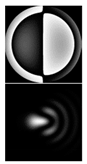
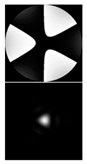
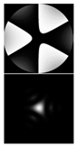
| Expansion Coefficients | Input Phase and PSF (Intensity) | ||
|---|---|---|---|
| α = 0.4 | α = 0.6 | α = 1 | |
 |  |  |  |
 |  |  |  |
 |  |  |  |
 |  |  | 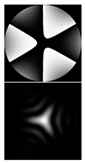 |
 |  |  |  |
 |  |  |  |
 |  |  |  |
 |  |  |  |
| l | 0 | 1 | 2 | 3 | 4 | 5 | 6 | 7 | 8 |
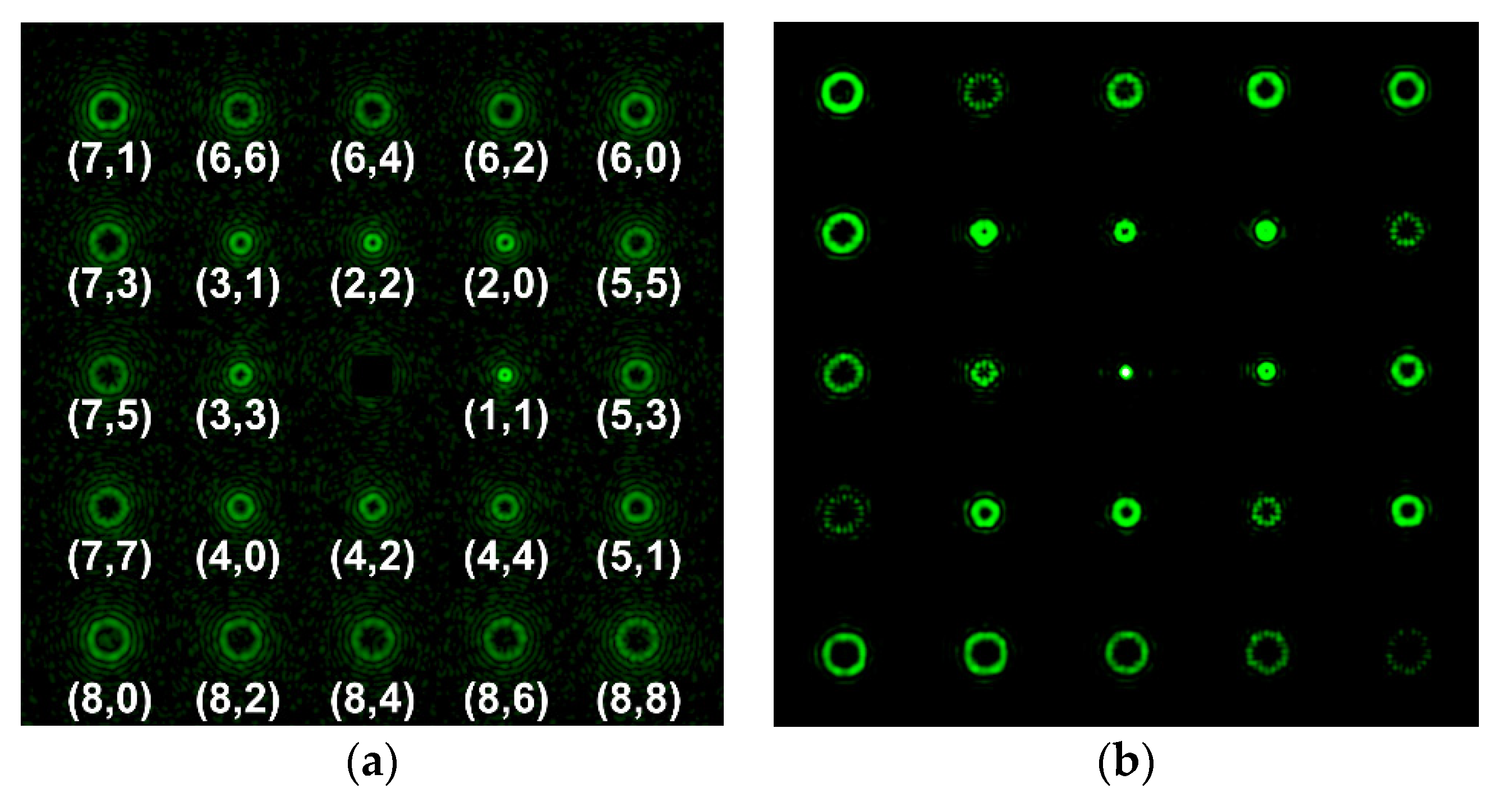
| (n, m) | (0, 0) | (1, 1) | (1, −1) | (2, 2) | (2, 0) | (2, −2) | (3, 3) | (3, 1) | (3, −1) |
| l | 9 | 10 | 11 | 12 | 13 | 14 | 15 | 16 | 17 |
| (n, m) | (3, −3) | (4, 4) | (4, 2) | (4, 0) | (4, −2) | (4, −4) | (5, 5) | (5, 3) | (5, 1) |
| l | 18 | 19 | 20 | 21 | 22 | 23 | 24 | 25 | 26 |
| (n, m) | (5, −1) | (5, −3) | (5, −5) | (6, 6) | (6, 4) | (6, 2) | (6, 0) | (6, −2) | (6, −4) |
| l | 27 | 28 | 29 | 30 | 31 | 32 | 33 | 34 | 35 |
| (n, m) | (6, −6) | (7, 7) | (7, 5) | (7, 3) | (7, 1) | (7, −1) | (7, −3) | (7, −5) | (7, −7) |
| l | 36 | 37 | 38 | 39 | 40 | 41 | 42 | 43 | 44 |
| (n, m) | (8, 8) | (8, 6) | (8, 4) | (8, 2) | (8, 0) | (8, −2) | (8, −4) | (8, −6) | (8, −8) |
| (n, m) | (n, m) | ||
|---|---|---|---|
| (0, 0) | 1 | (4, 0) | |
| (1, 1) | (4, 2) | ||
| (2, 0) | (4, 4) | ||
| (2, 2) | (5, 1) | ||
| (3, 1) | (5, 3) | ||
| (3, 3) | (5,5) |
© 2020 by the authors. Licensee MDPI, Basel, Switzerland. This article is an open access article distributed under the terms and conditions of the Creative Commons Attribution (CC BY) license (http://creativecommons.org/licenses/by/4.0/).
Share and Cite
Khonina, S.N.; Karpeev, S.V.; Porfirev, A.P. Wavefront Aberration Sensor Based on a Multichannel Diffractive Optical Element. Sensors 2020, 20, 3850. https://doi.org/10.3390/s20143850
Khonina SN, Karpeev SV, Porfirev AP. Wavefront Aberration Sensor Based on a Multichannel Diffractive Optical Element. Sensors. 2020; 20(14):3850. https://doi.org/10.3390/s20143850
Chicago/Turabian StyleKhonina, Svetlana N., Sergey V. Karpeev, and Alexey P. Porfirev. 2020. "Wavefront Aberration Sensor Based on a Multichannel Diffractive Optical Element" Sensors 20, no. 14: 3850. https://doi.org/10.3390/s20143850
APA StyleKhonina, S. N., Karpeev, S. V., & Porfirev, A. P. (2020). Wavefront Aberration Sensor Based on a Multichannel Diffractive Optical Element. Sensors, 20(14), 3850. https://doi.org/10.3390/s20143850