Performing Calibration of Transmittance by Single RGB-LED within the Visible Spectrum

 ,
,  ,
,
Abstract
1. Introduction
2. Materials and Methods
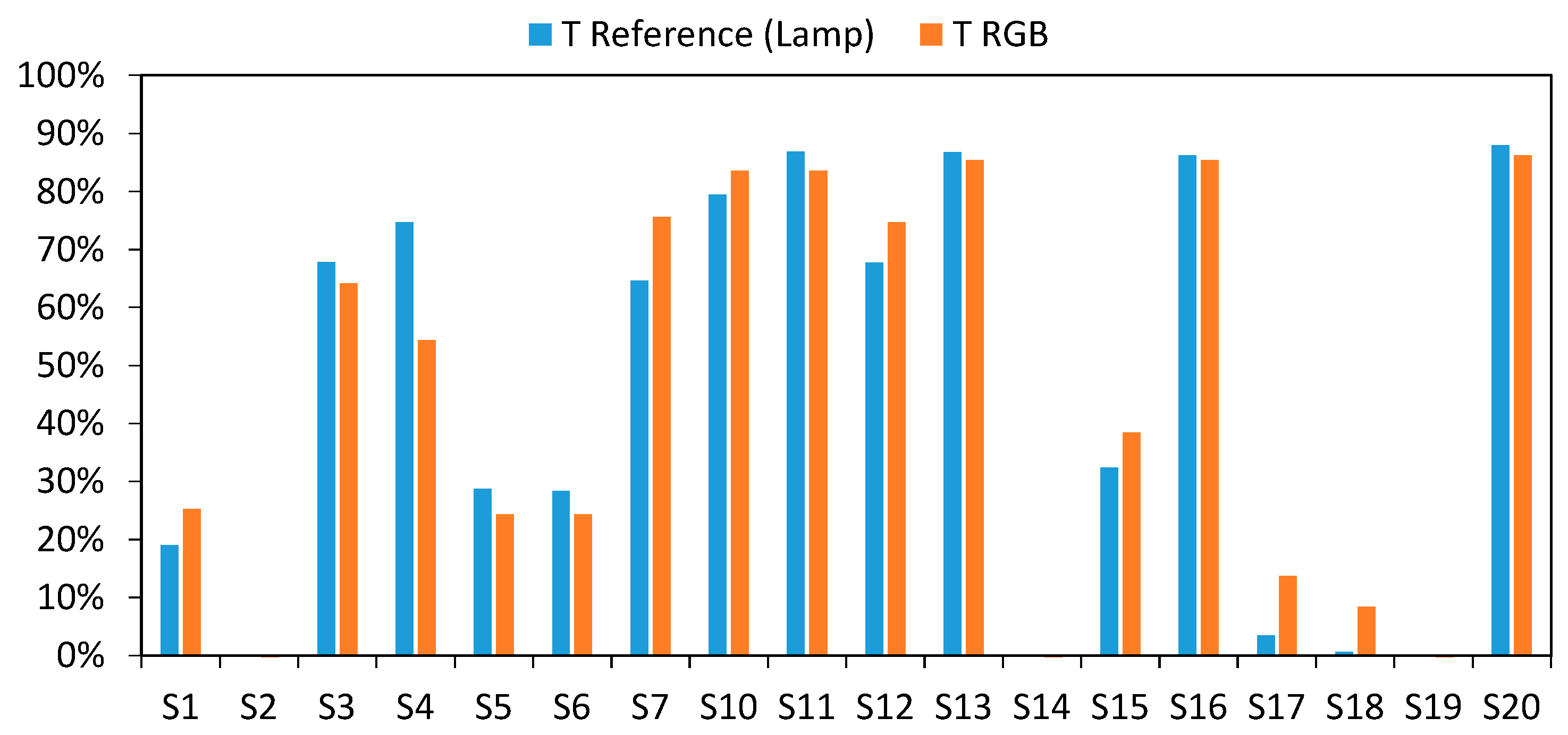
2.1. Analyzed Samples
2.2. Reference Equipment
- ISO 22891: 2013: Determination of transmittance by diffuse reflectance measurement.
- ISO 10110-9: 2016: Preparation of drawings for optical elements and systems—Part 9: Surface treatment and coating.
- ISO 7887:2011: Water Quality—Examination and determination of color.
- ISO 9001 7.6: Control of monitoring and measuring equipment.
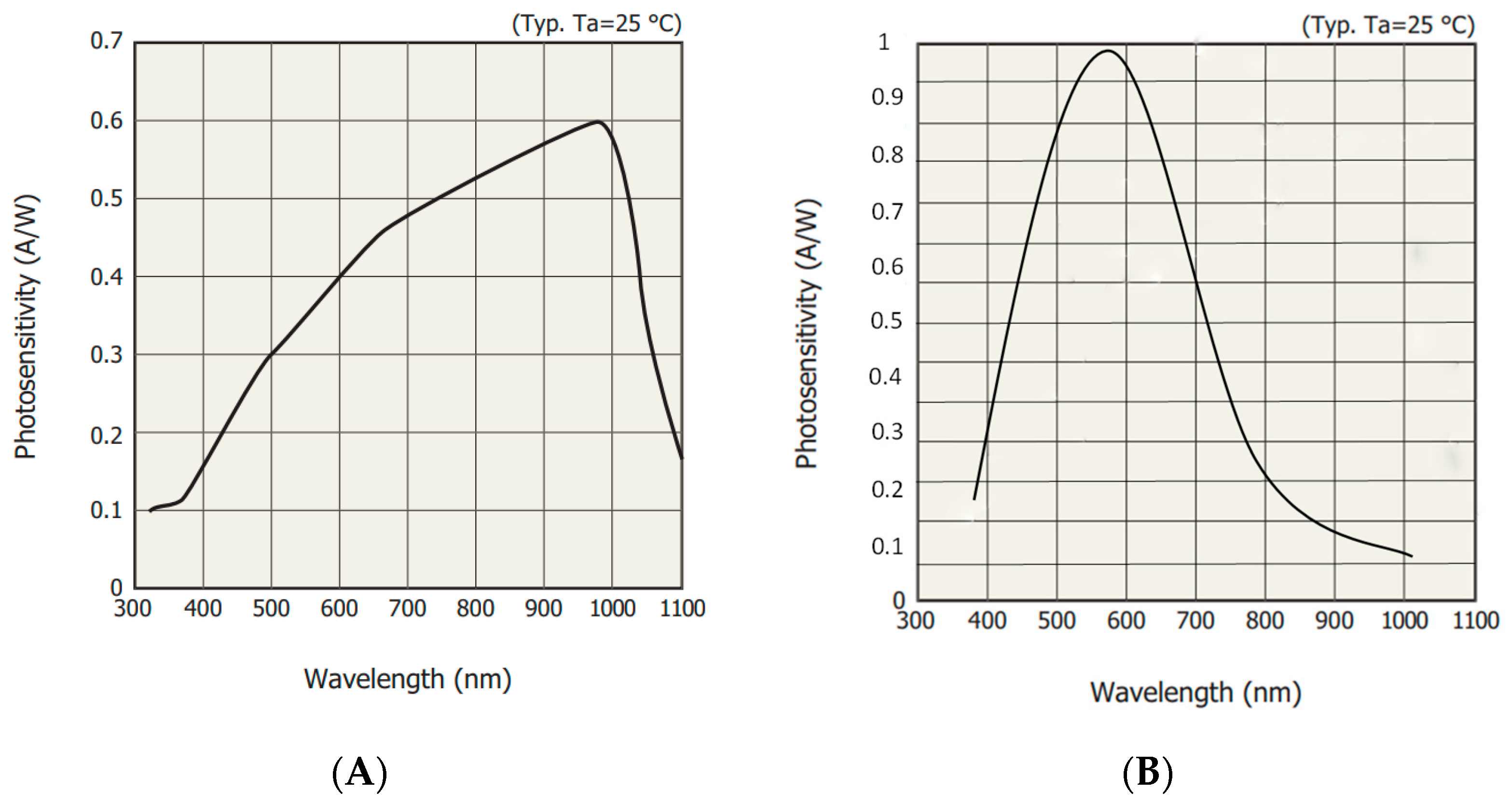
2.3. Sensor Unit
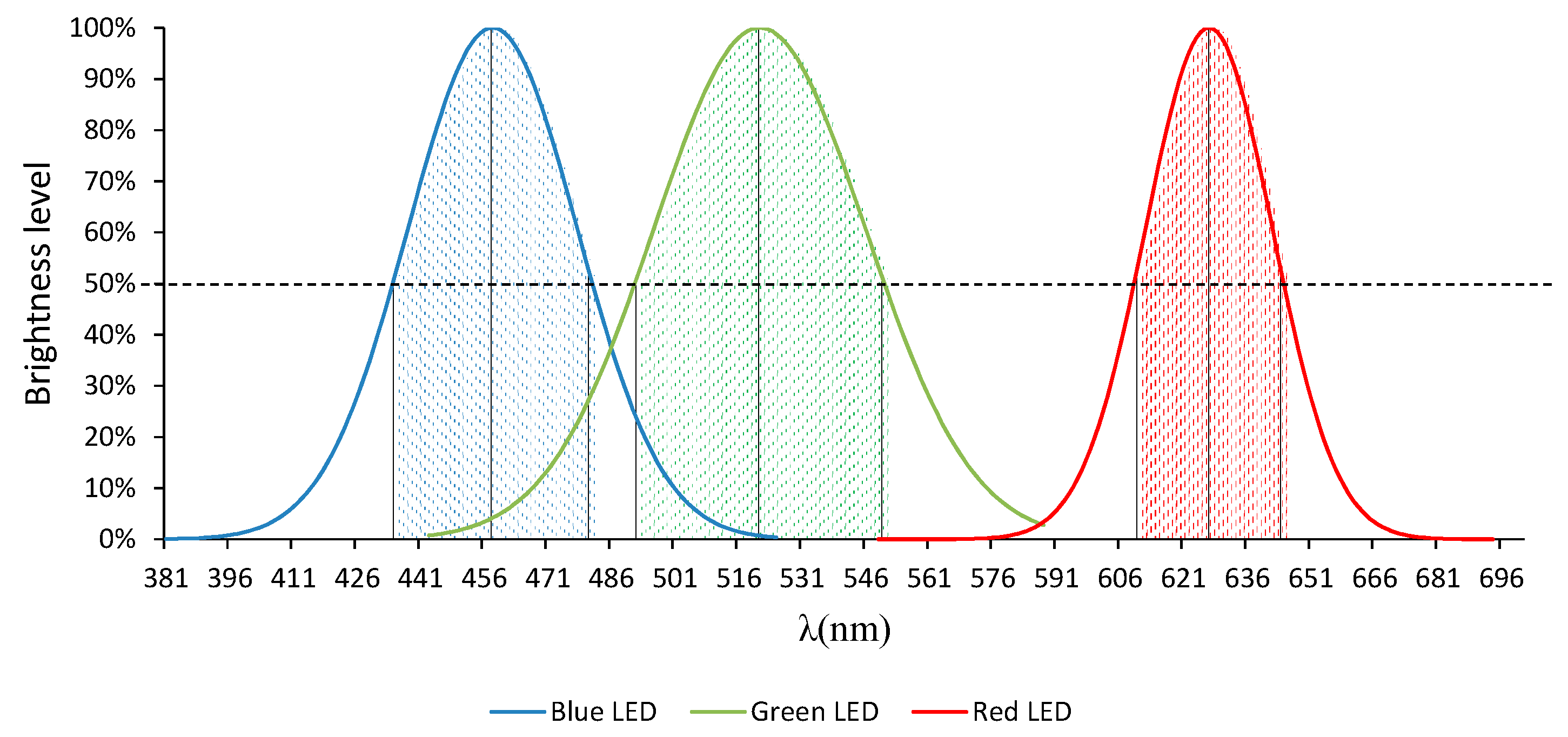
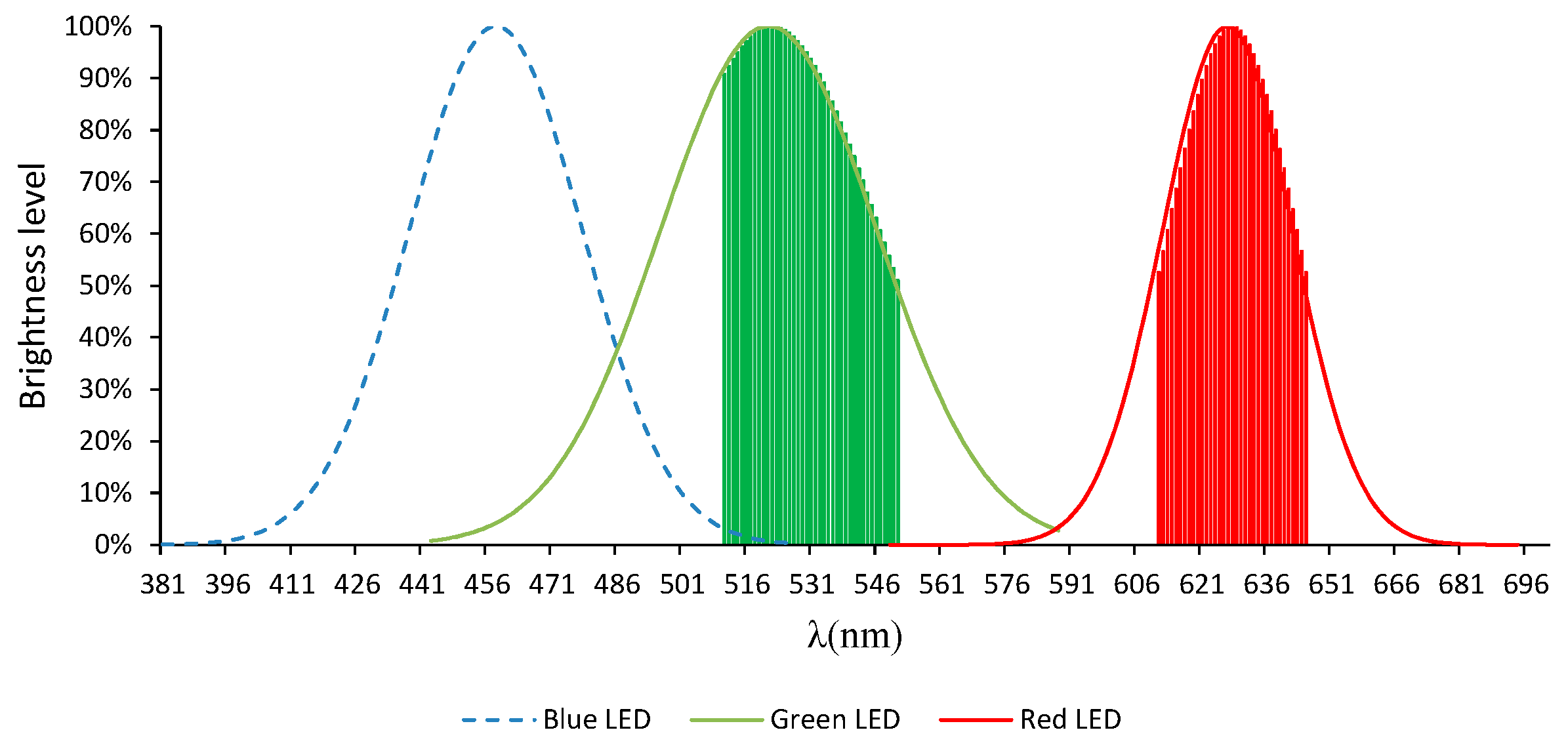
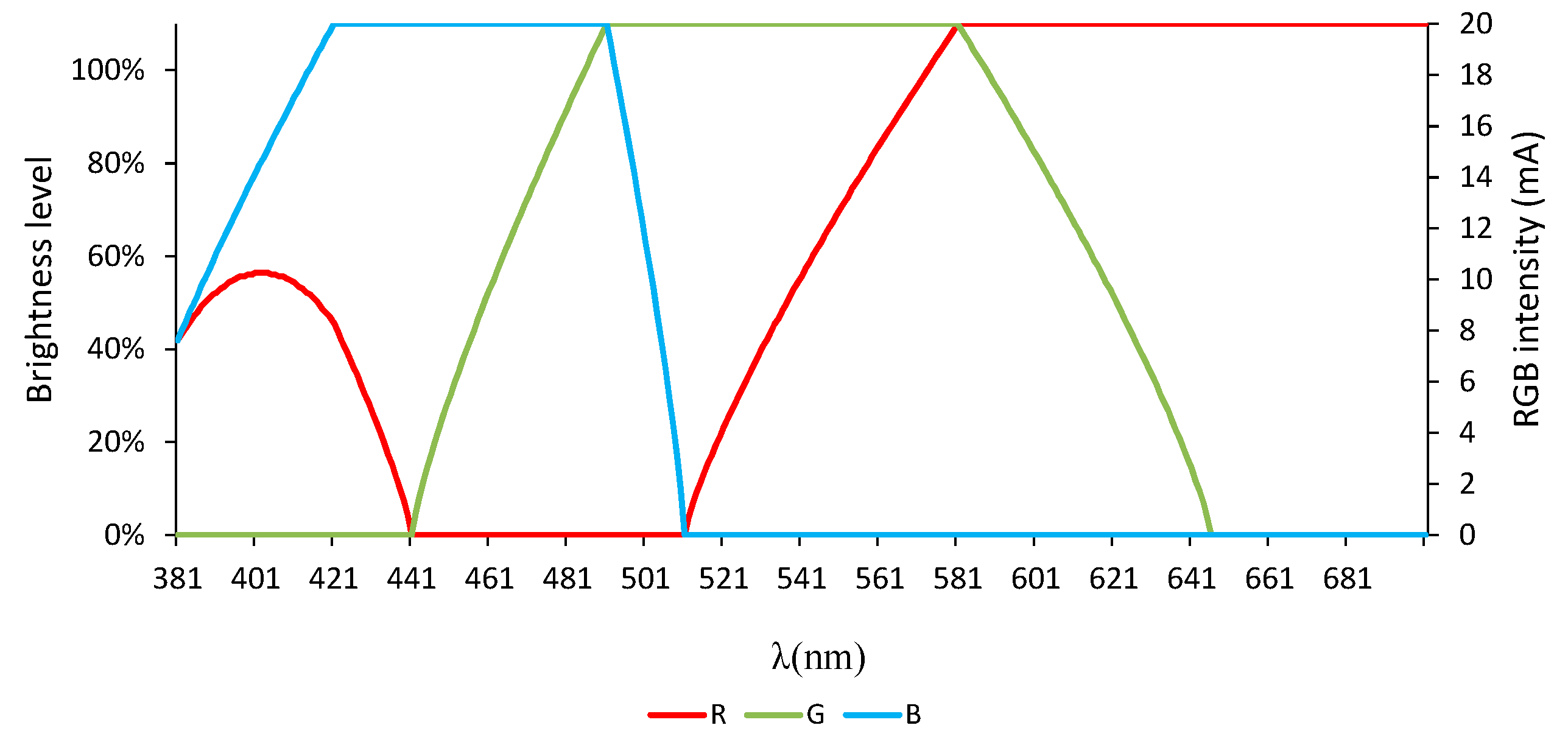
2.4. RGB Light-Emitting Diode (RGB-LED)
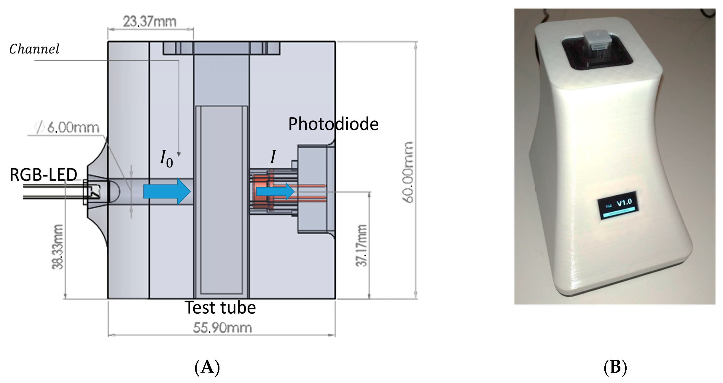
2.5. Hardware
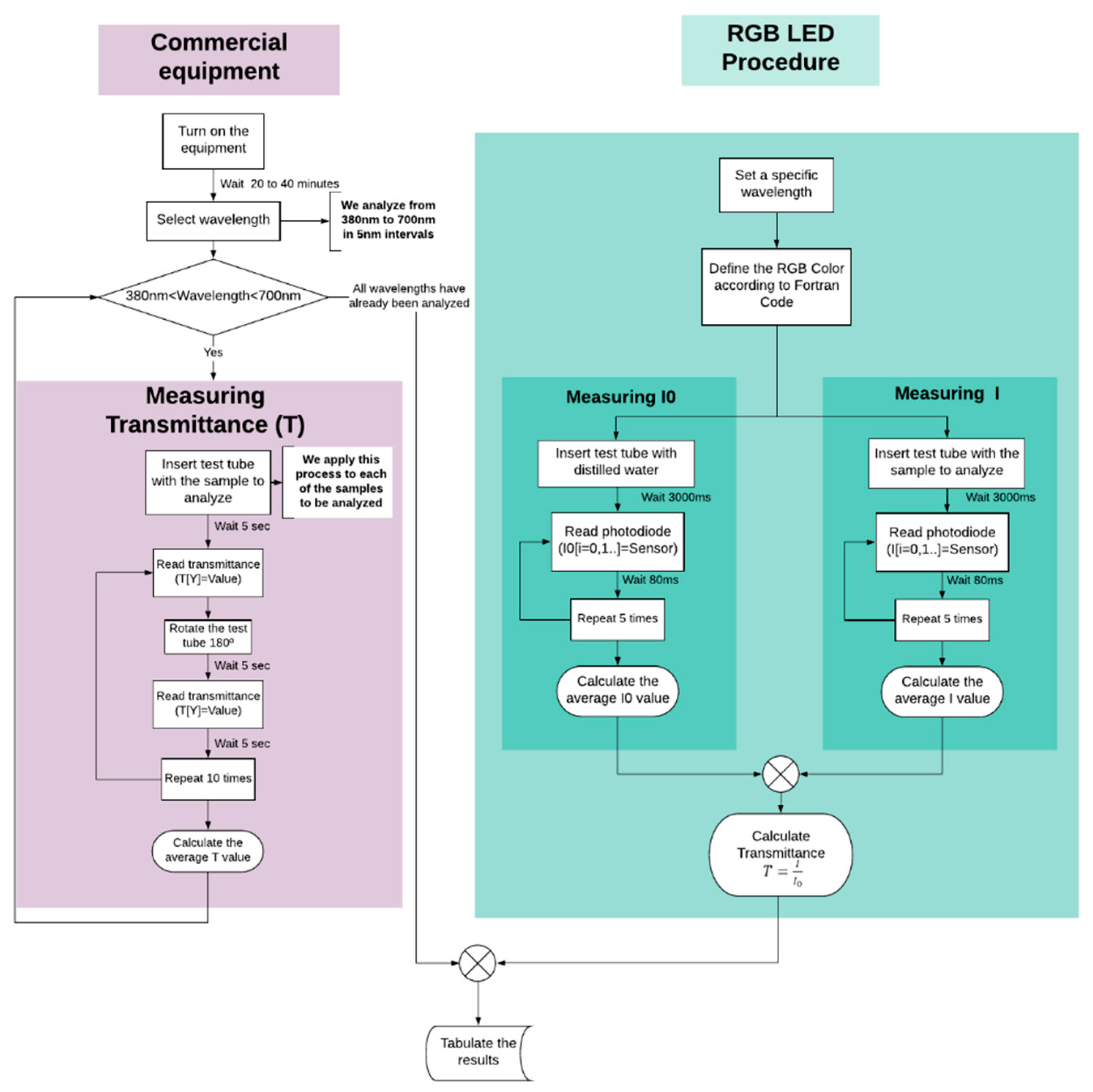
2.6. Methodology
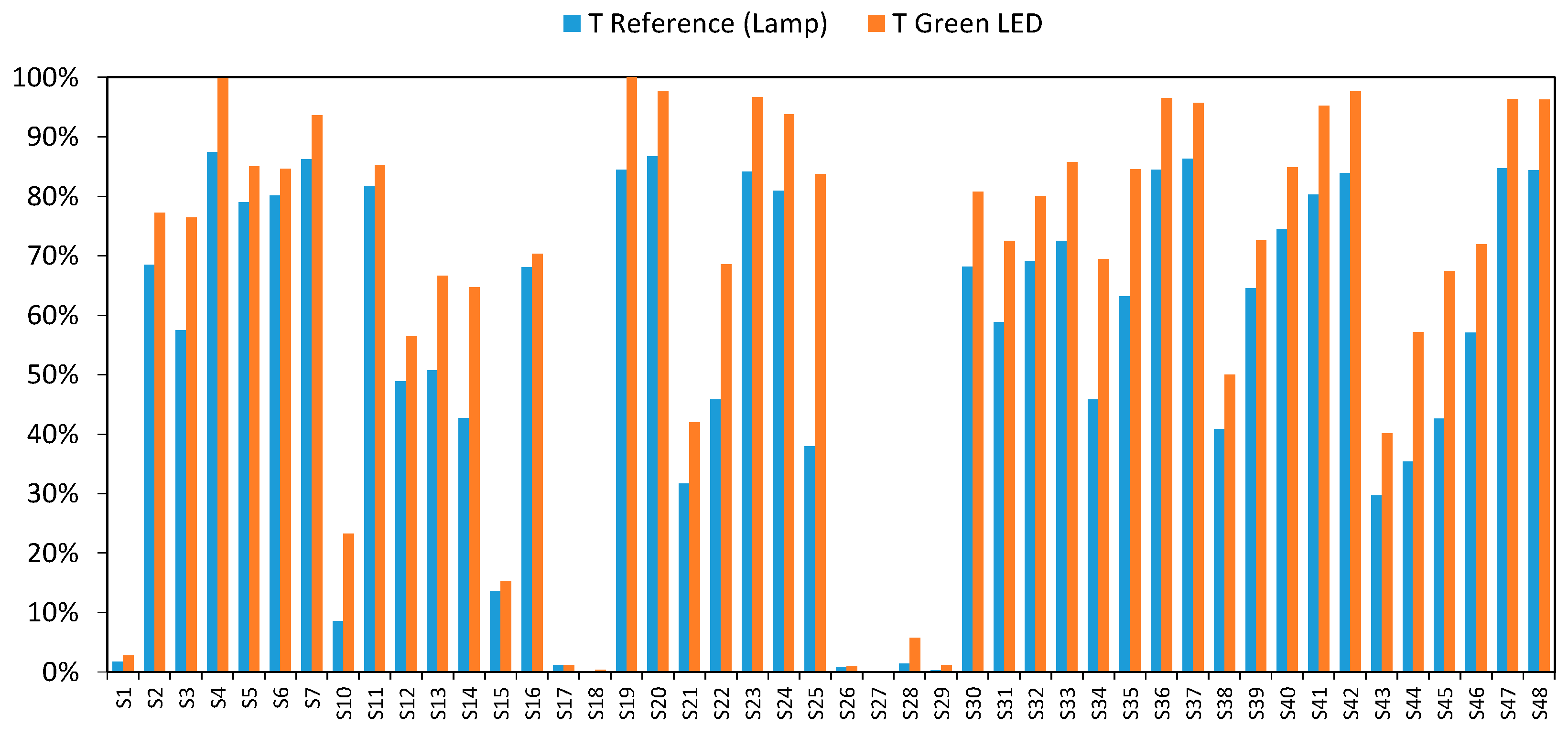
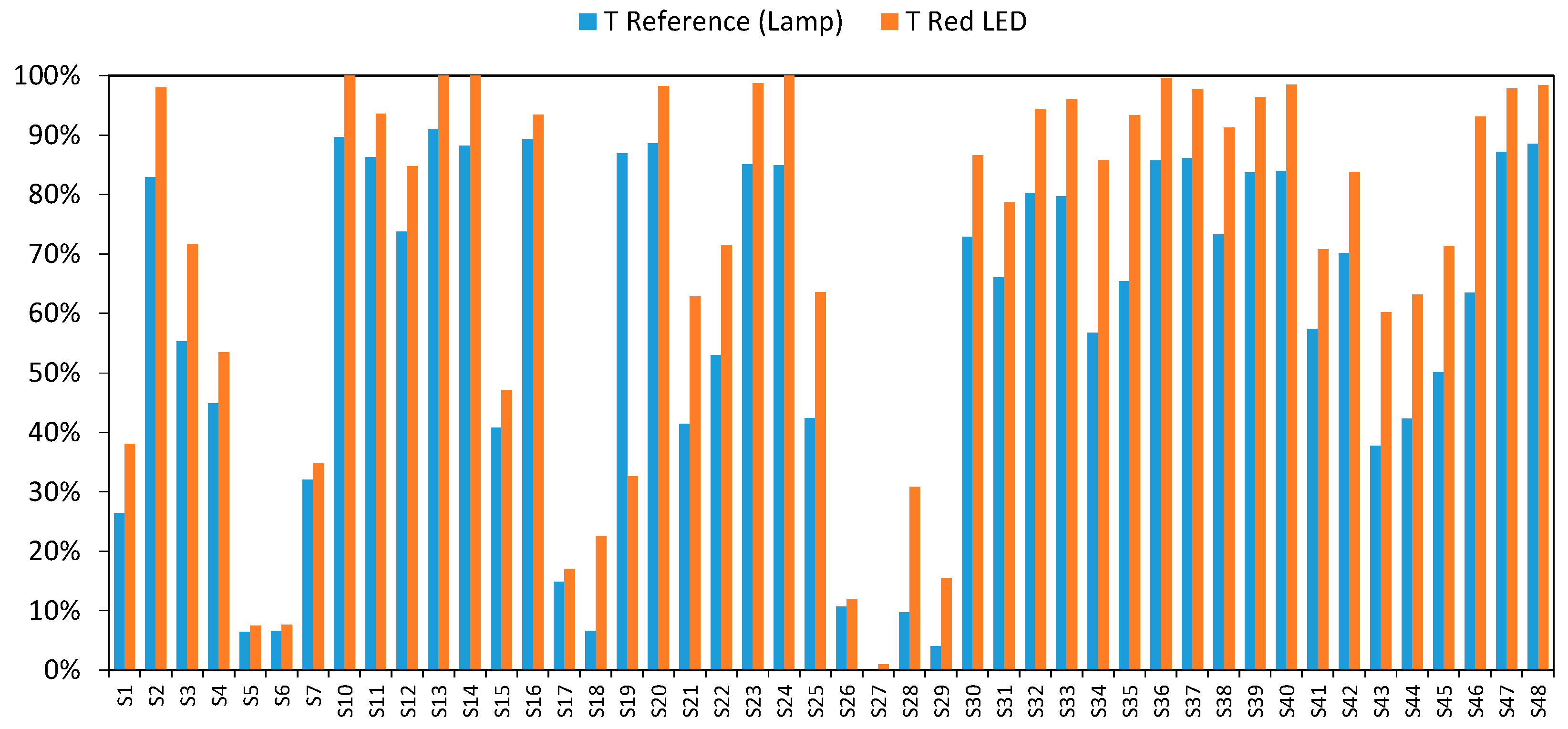
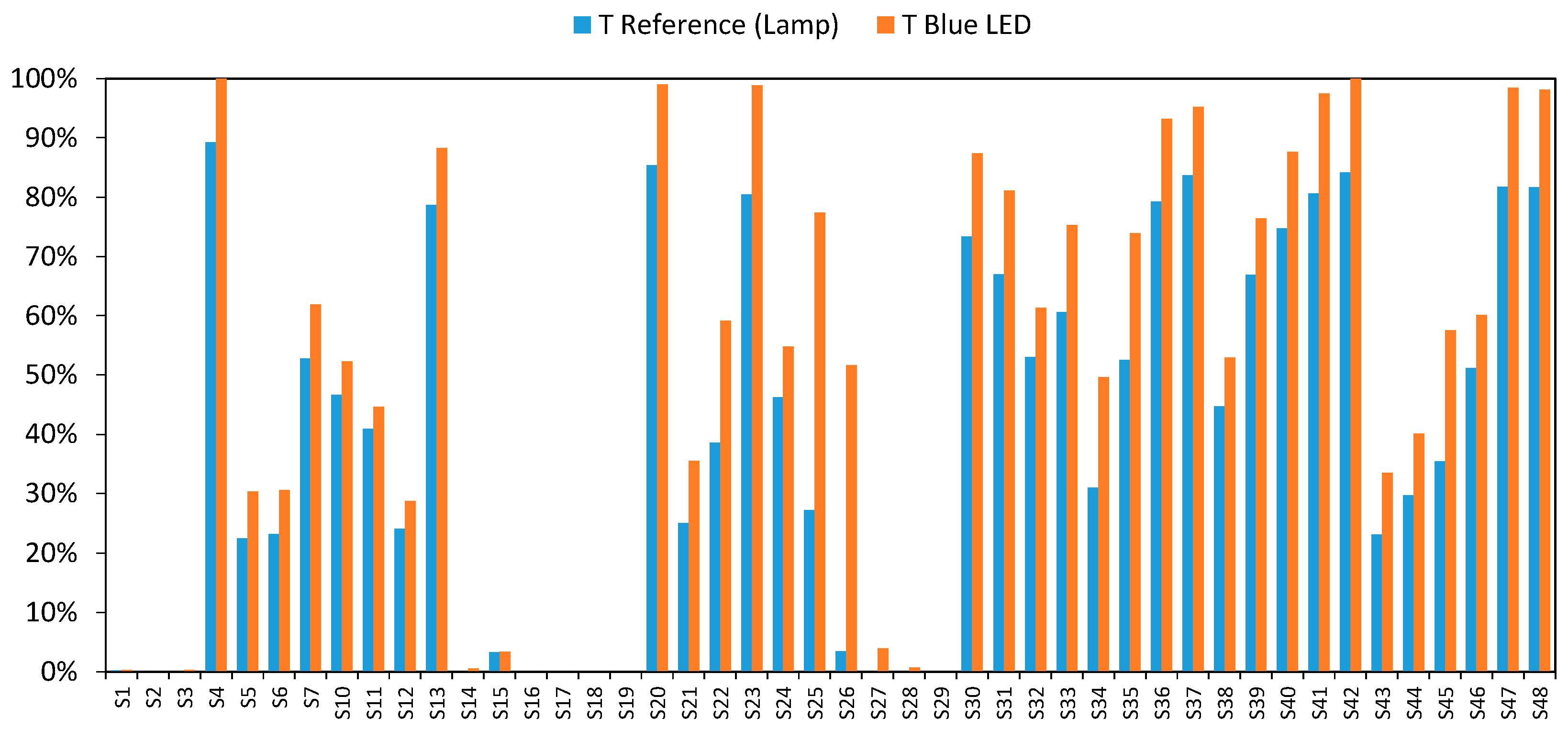
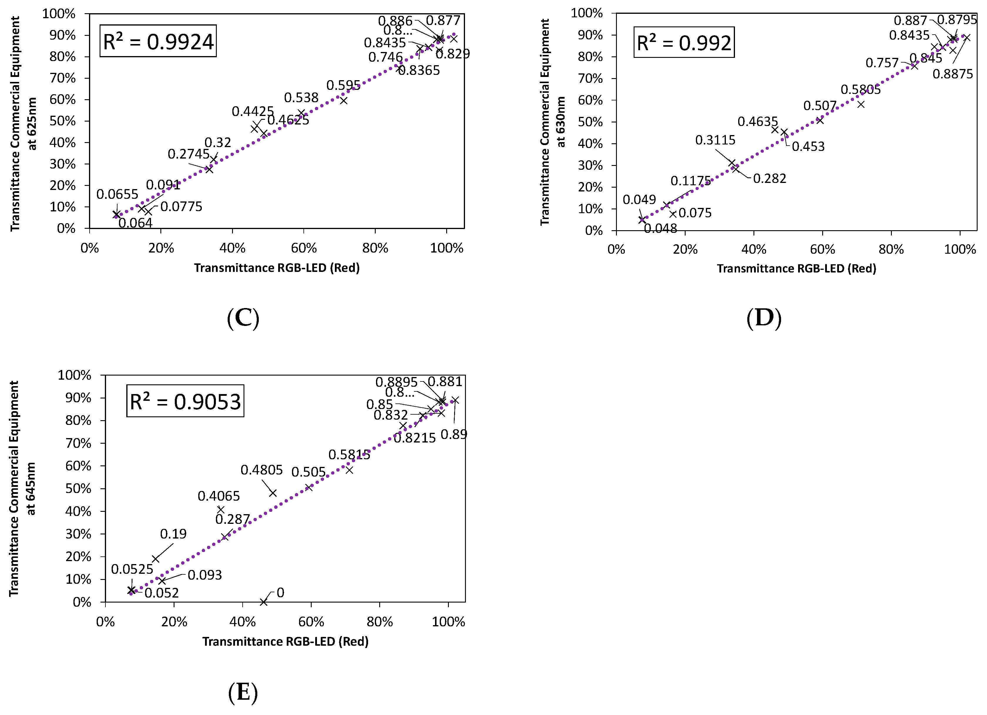
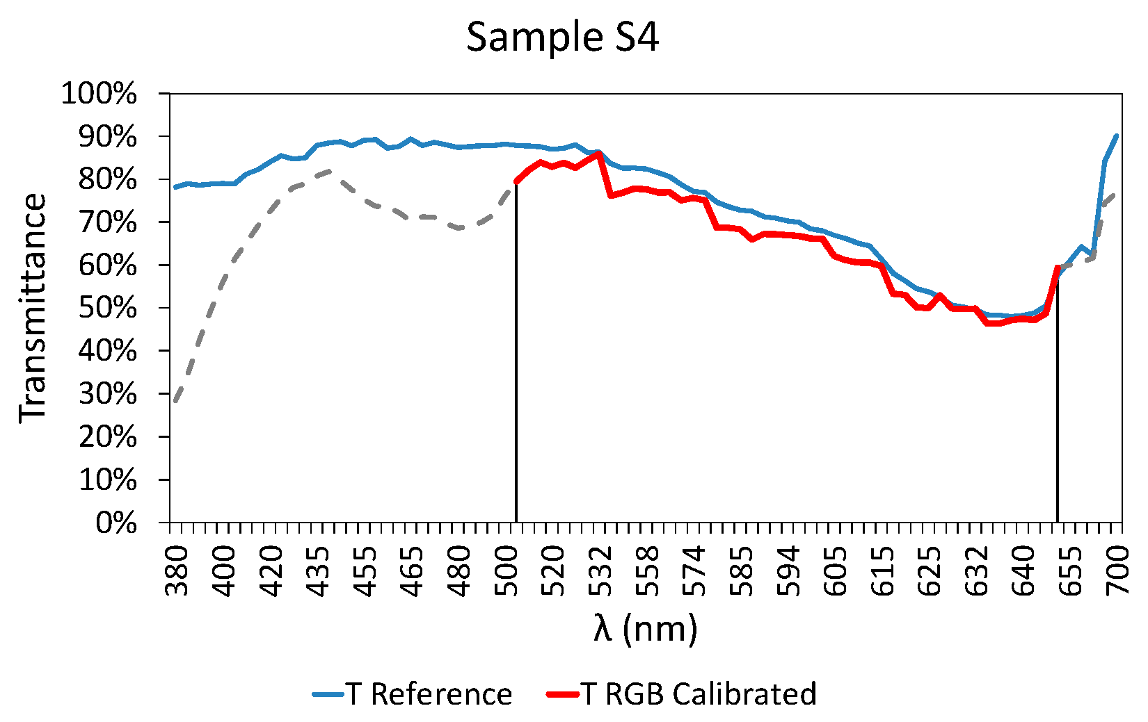
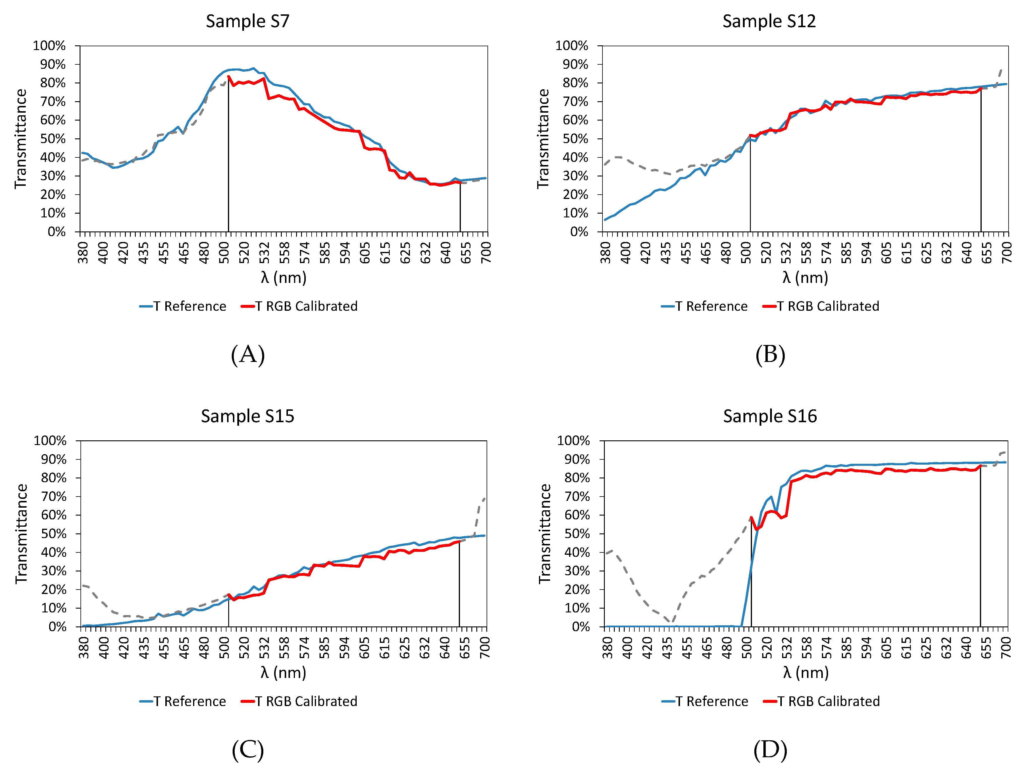
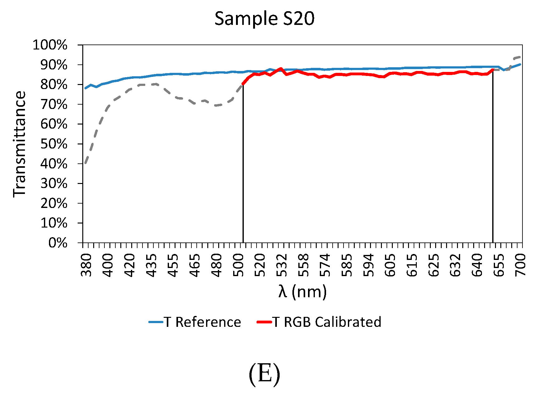
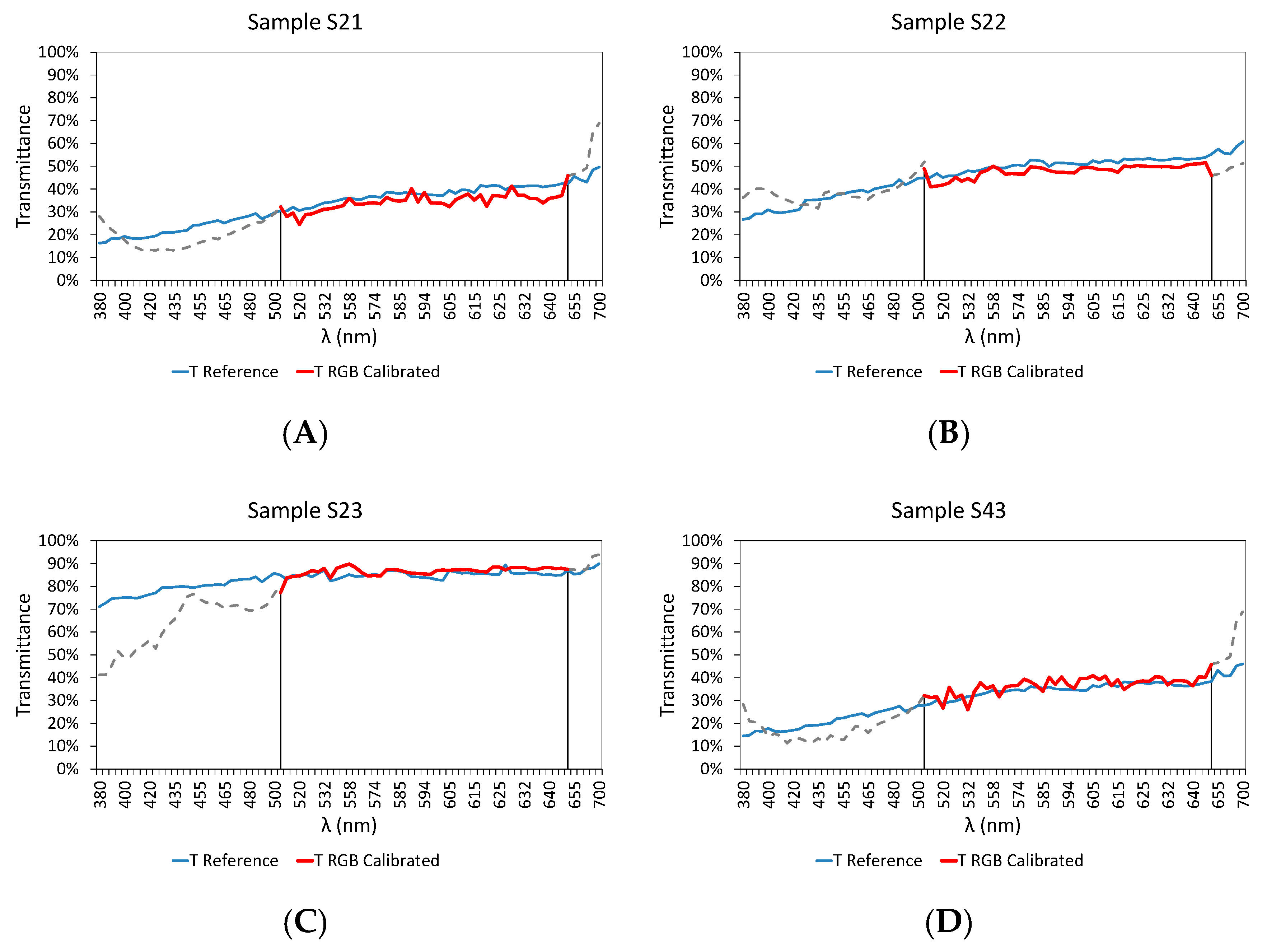
3. Results and Discussion
3.1. Preliminary Tests
3.2. Extension of the Working Range
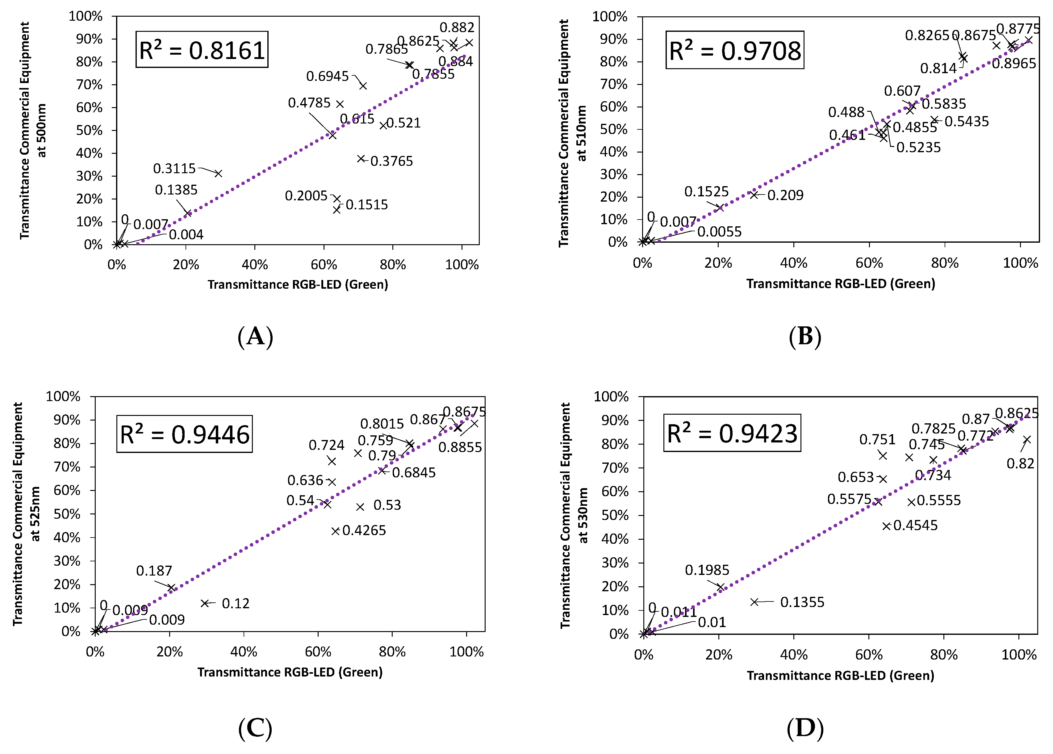
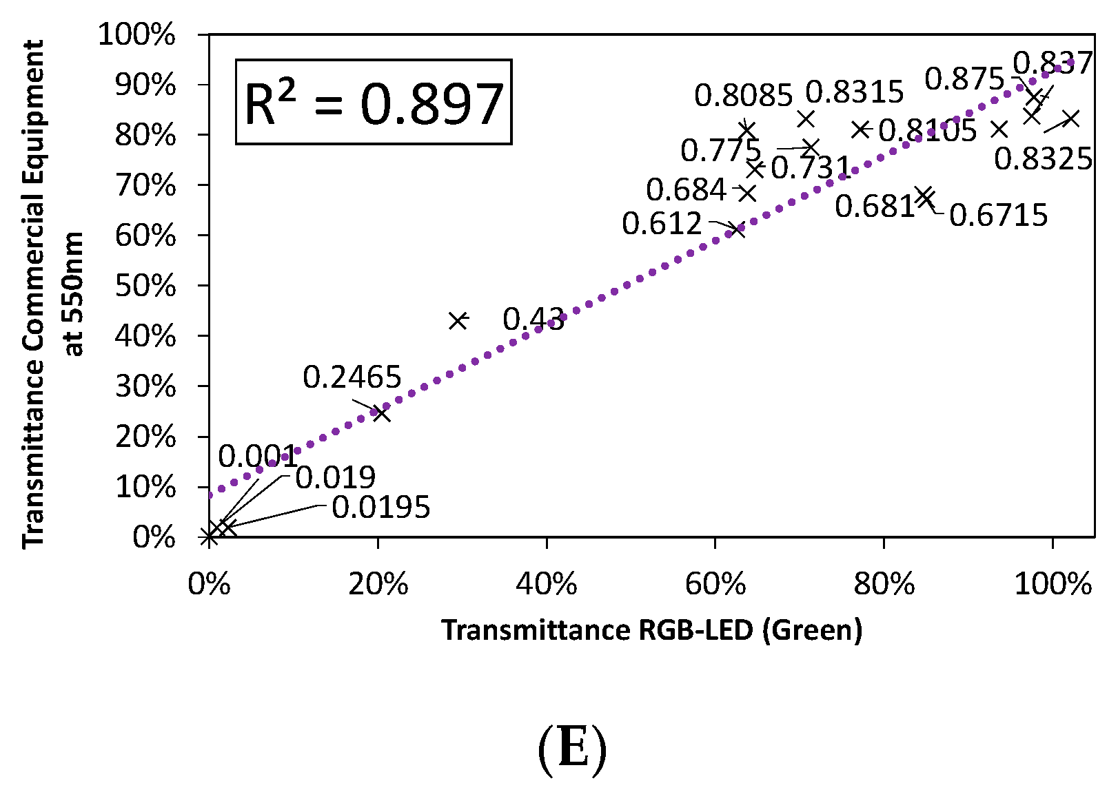
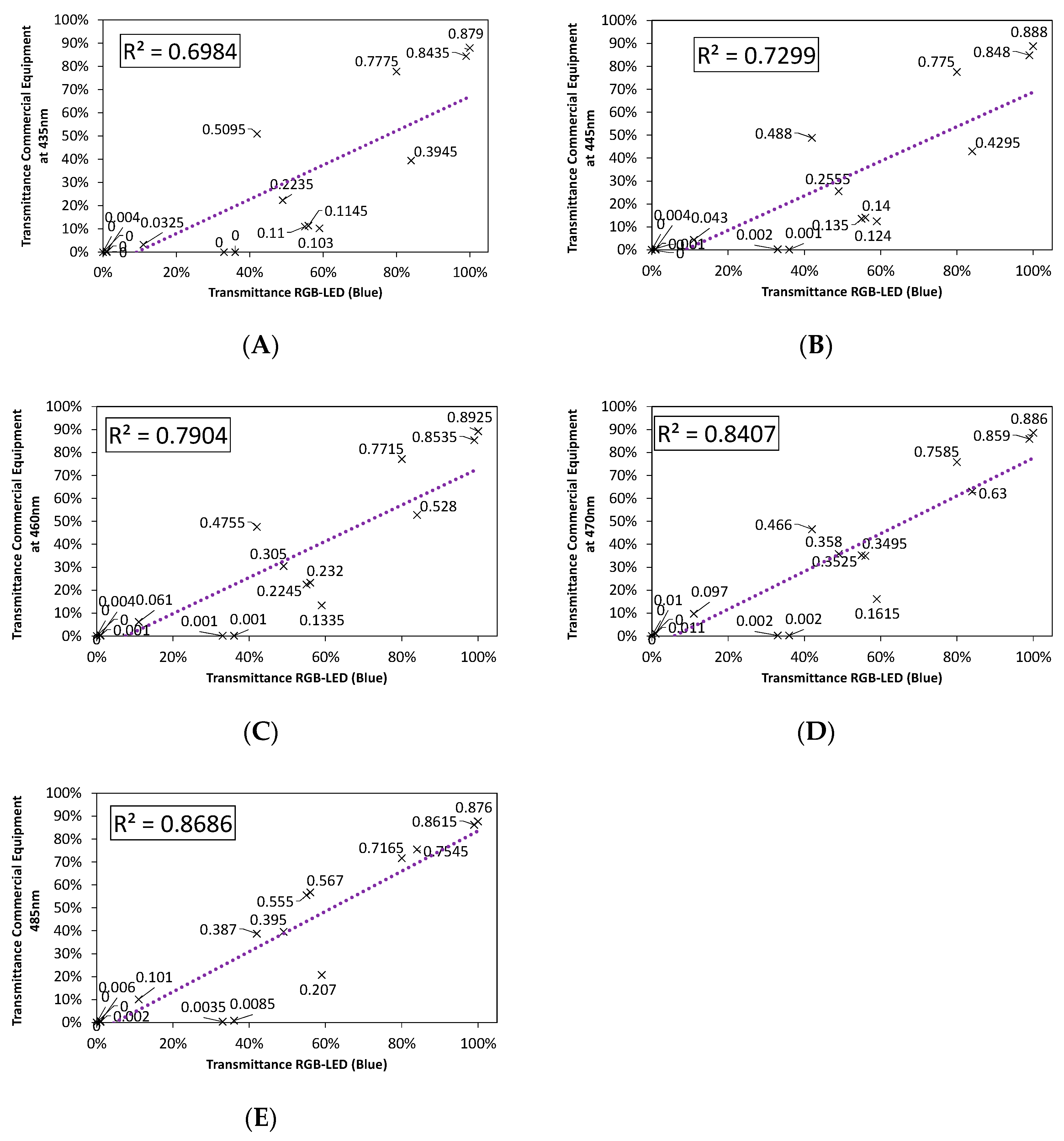
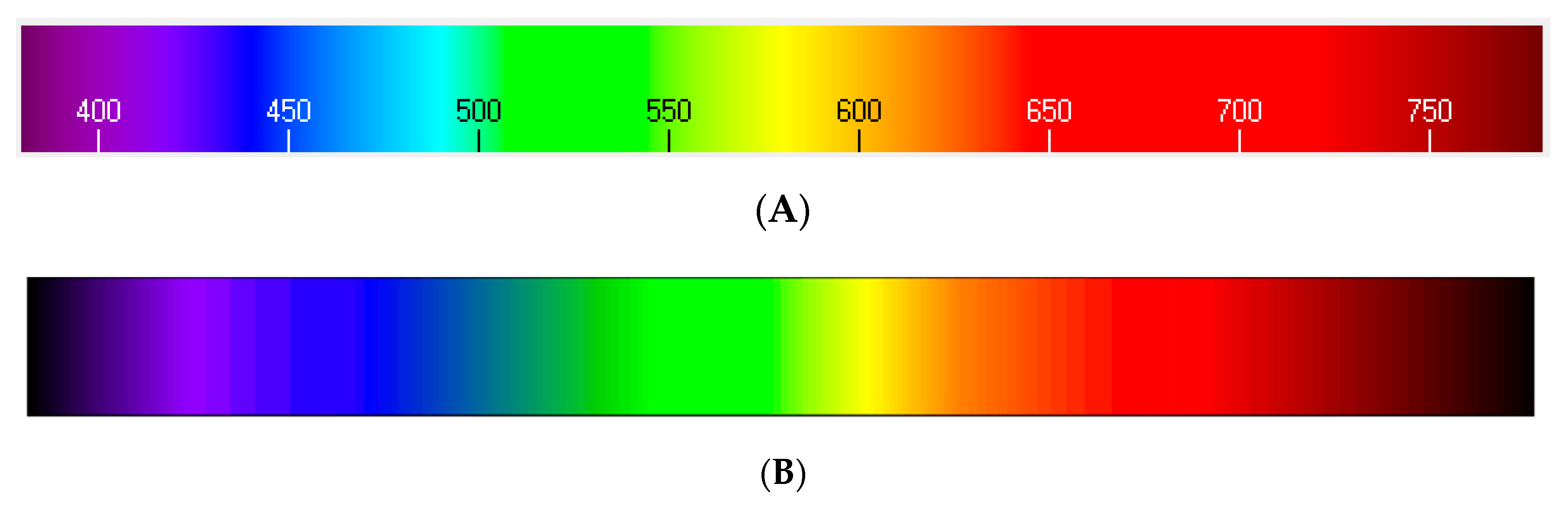
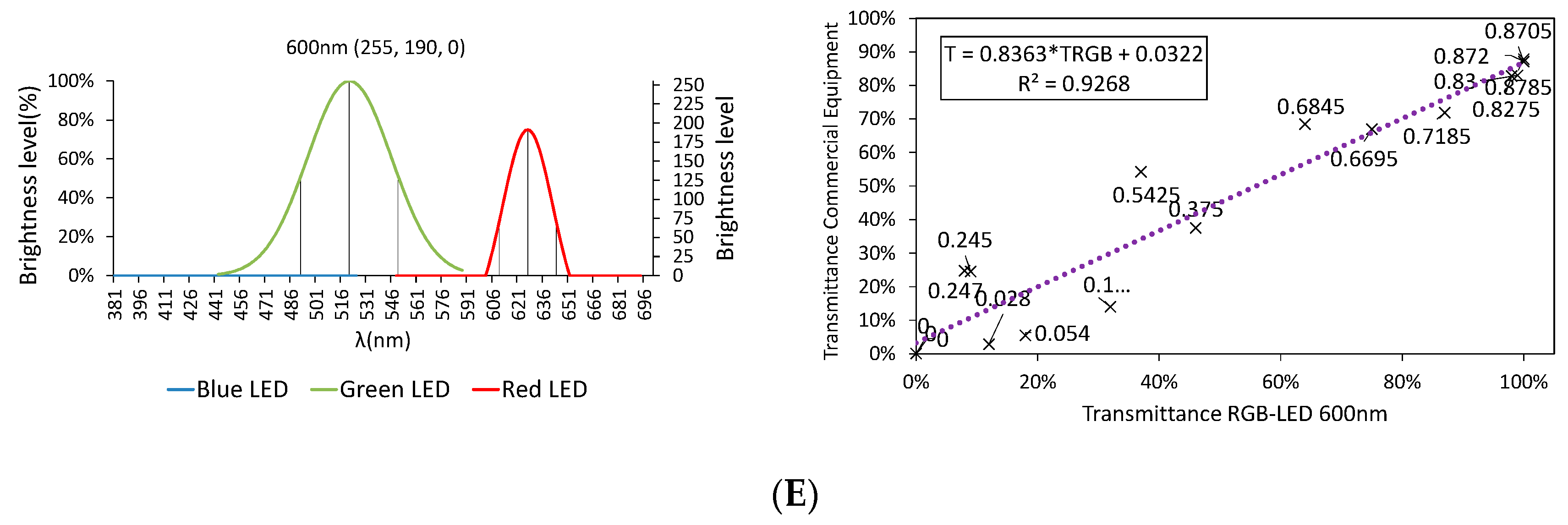
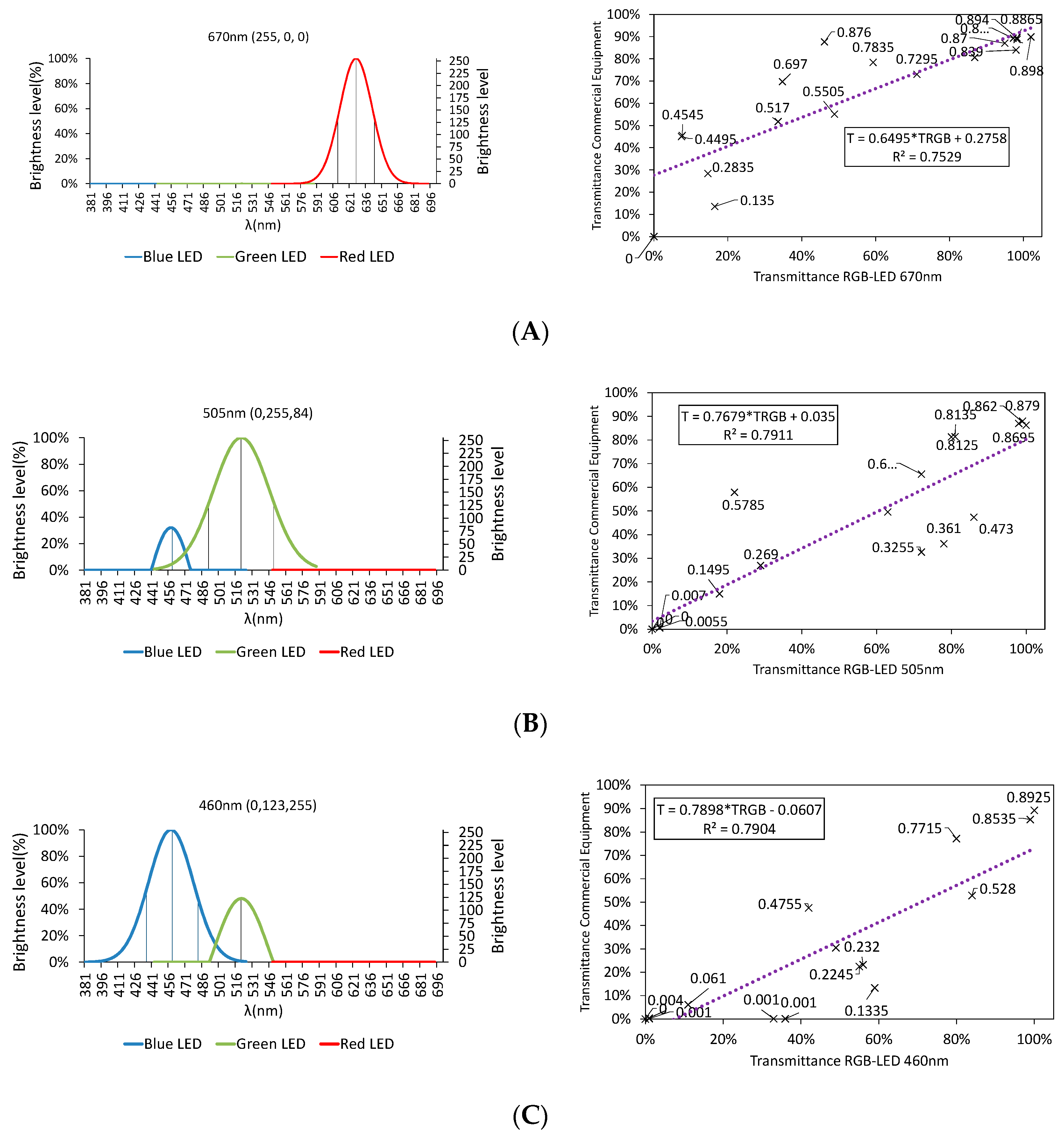
3.2.1. Color Rendering
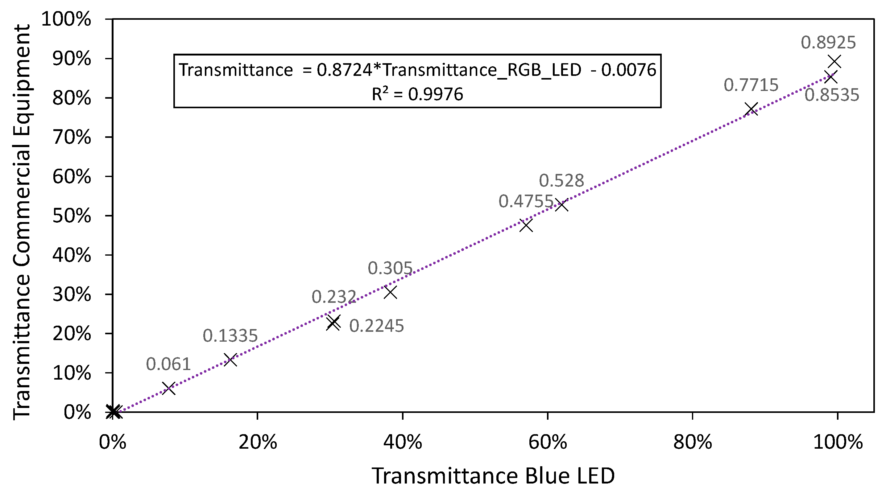
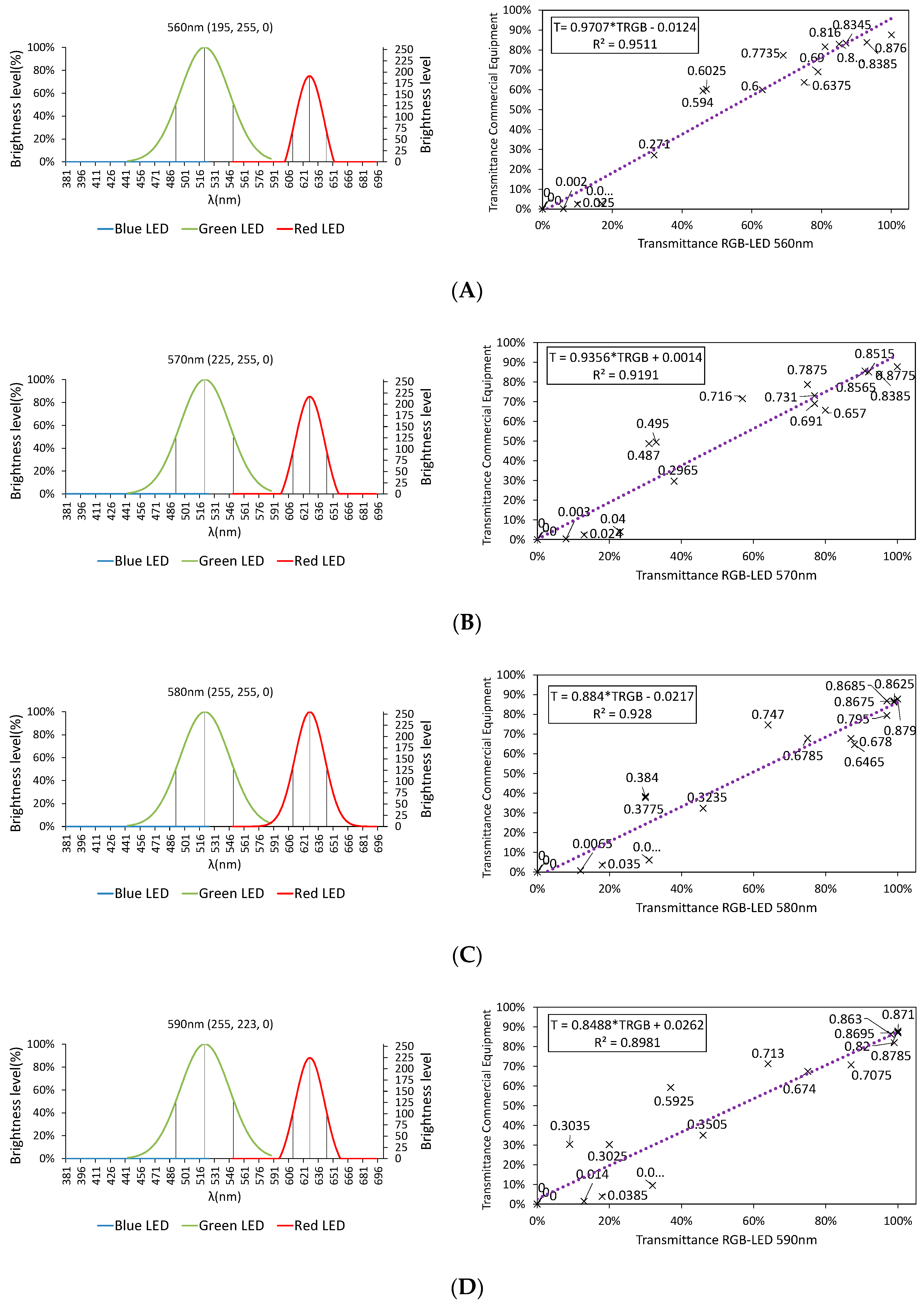
3.2.2. LED Combination Calibration
3.3. Final Results
4. Conclusions
- (i)
- Demonstrates that RGB-LED can be used to carry out a spectral analysis of wastewater, obtaining results very close to those provided by commercial equipment based on incandescent lamps.
- (ii)
- Develops a calibration system for measuring transmittance values between 510 and 645 nm using a single RGB-LED, with high accuracy. Moreover, it enables us to reduce the number of elements used, and therefore, significantly reduce the cost of the equipment.
- (iii)
- Models the transmittance value of a specific wavelength without the need for optical elements, such as monochromators or diffraction gratings.
- (iv)
- Uses the red and green LEDs in combination to model those parts of the visible spectrum that cannot be modelled by the RGB-LED when each of the LEDs that composes it acts individually. This allows the wavelength range to be extended without increasing the number of LEDs used.
- (v)
- Achieves reductions in the dimensions, costs, and sampling times of the equipment, which are vital aspects for the development of low-cost autonomous systems designed to measure in any type of environment.
Author Contributions
Funding
Acknowledgments
Conflicts of Interest
References
- Rakedjian, B. StormWater Overflows Challenges. In Proceedings of the 12th EWA Brussels Conference EU Water Policy and Sustainable Development, Brussels, Belgium, 8 November 2016. [Google Scholar]
- Ward, S.; Butler, D. Compliance with the Urban Waste Water Treatment Directive: European Union City Responses in Relation to Combined Sewer Overflow Discharges; University of Exeter: Exeter, UK, 2009. [Google Scholar]
- Del Río Cambeses, H. Estudio de los Flujos de Contaminación Movilizados en Tiempo de Lluvia y Estrategias de Gestión en un Sistema de Saneamiento y Drenaje unitario de una Cuenca Urbana Densa de la España Húmeda. Ph.D. Thesis, Universidade da Coruña, A Coruña, Spain, 2011. [Google Scholar]
- García, J.T.; Espín-Leal, P.; Vigueras-Rodriguez, A.; Castillo, L.G.; Carrillo, J.M.; Martínez-Solano, P.D.; Nevado-Santos, S. Urban Runoff Characteristics in Combined Sewer Overflows (CSOs): Analysis of Storm Events in Southeastern Spain. Water 2017, 9, 303. [Google Scholar] [CrossRef]
- García, J.T.; Espín-Leal, P.; Vigueras-Rodríguez, A.; Carrillo, J.M.; Castillo, L.G. Synthetic Pollutograph by Prediction Indices: An Evaluation in Several Urban Sub-Catchments. Sustainability 2018, 10, 2634. [Google Scholar] [CrossRef]
- Puertas-Agudo, J.; Suárez-López, J.; Anta-Álvarez, J. Gestión de las Aguas Pluviales. Implicaciones en el Diseño de Sistemas de Saneamiento y Drenaje Urbano; CEDEX: Madrid, Spain; Ministerio de Fomento Información Administrativa: Madrid, Spain, 2008. [Google Scholar]
- Naves, J.; Jikia, Z.; Anta, J.; Puertas, J.; Suárez, J.; Regueiro-Picallo, M. Experimental study of pollutant washoff on a full-scale street section physical model. Water Sci. Technol. 2017, 76, 2821–2829. [Google Scholar] [CrossRef] [PubMed]
- Anta, J.; Cagiao, J.; Suárez, J.; Peña, E. Análisis de la movilización de sólidos en suspensión en una cuenca urbana separativa mediante la aplicación del muestreo en continuo de la turbidez. Ing. Agua 2009, 16, 189–200. [Google Scholar] [CrossRef]
- Gruber, G.; Winkler, S.; Pressl, A. Continuous monitoring in sewer networks an approach for quantification of pollution loads from CSOs into surface water bodies. Water Sci. Technol. 2005, 52, 215–223. [Google Scholar] [CrossRef]
- Irvine, K.N.; McCorkhill, G.; Caruso, J. Continuous monitoring of conventional parameters to assess receiving water quality in support of combined sewer overflow abatement plans. Water Environ. Res. 2005, 77, 543–552. [Google Scholar] [CrossRef]
- Ellis, J.B.; Hvitved-Jacobsen, T. Urban drainage impacts on receiving waters. J. Hydraul. Res. 1996, 34, 771–783. [Google Scholar] [CrossRef]
- Copeland, C. Clean Water Act: A Summary of the Law; Congressional Research Service, Library of Congress: Washington, DC, USA, 1999.
- USA Environmental Protection Agency. Clean Water Act; EPA: Washington, DC, USA, 2008.
- Métadier, M.; Bertrand-Krajewski, J.L. The use of long-term on-line turbidity measurements for the calculation of urban stormwater pollutant concentrations, loads, pollutographs and intra-event fluxes. Water Res. 2012, 46, 6836–6856. [Google Scholar] [CrossRef]
- Van den Broeke, J.; Langergraber, G.; Weingartner, A. On-line and in-situ UV/vis spectroscopy for multi-parameter measurements: A brief review. Spectrosc. Eur. 2006, 18, 15–18. [Google Scholar]
- Malgrat, P.; Sunyer, D.; Russo, B. Las Nuevas Exigencias Sobre las Explotaciones de Saneamiento Derivadas de la Aplicación del Real Decreto 1290/2012. Available online: https://www.um.es/documents/3456781/14232816/Monitorizaci%C3%83%C2%B3n+y+Evaluaci%C3%83%C2%B3n+ciudad+de+Murcia_Juan+T_Garcia.pdf/af5f1070-6843-4929-b9db-e215ebe8c86f (accessed on 20 June 2020).
- Kallis, G.; Butler, D. The EU water framework directive: Measures and implications. Water Policy 2001, 3, 125–142. [Google Scholar] [CrossRef]
- Caradot, N. Continous Monitoring of Combined Sewer Overflows in the Sewer and the Receiving River; Kompetenzzentrum Wasser Berlin gGmbH: Berlin, Germany, 2013. [Google Scholar]
- Sandoval, S.; Torres, A.; Pawlowsky-Reusing, E.; Riechel, M.; Caradot, N. The evaluation of rainfall influence on combined sewer overflows characteristics: The Berlin case study. Water Sci. Technol. 2013, 68, 2683–2690. [Google Scholar] [CrossRef] [PubMed]
- Murphy, K.; Heery, B.; Sullivana, T.; Zhang, D.; Paludetti, L.; Lau, K.T.; Diamond, D.; Costa, E.; O’Connor, N.; Regan, F. A low-cost autonomous optical sensor for water quality monitoring. Talanta 2015, 132, 520–527. [Google Scholar] [CrossRef] [PubMed]
- Wego, A. Accuracy simulation of an LED based spectrophotometer. Opt. Int. J. Light Electron Opt. 2013, 124, 644–649. [Google Scholar] [CrossRef]
- Schnable, J.G.; Grochowski, P.J.; Wilhelm, L.; Harding, C.; Kiefer, M.; Orr, R.S. Portable LED-array VIS–NIR spectrophotometer/nephelometer. Field Anal. Chem. Technol. 1998, 2, 21–28. [Google Scholar] [CrossRef]
- Rocha, F.R.; Martelli, P.B.; Reis, B.F. Simultaneous in-line concentration for spectrophotometric determination of cations and anions. J. Braz. Chem. Soc. 2004, 15, 38–42. [Google Scholar] [CrossRef]
- Venugopalan, H. UVC LEDs enable cost-effective spectroscopic instruments. Laser Focus World 2015, 51, 81–85. [Google Scholar]
- Carreres-Prieto, D.; García, J.T.; Cerdán-Cartagena, F.; Suardiaz-Muro, J. Spectroscopy Transmittance by LED Calibration. Sensors 2019, 19, 2951. [Google Scholar] [CrossRef]
- Benavides, M.; Mailier, J.; Hantson, A.L.; Muñoz, G.; Vargas, A.; Van Impe, J.; Vande Wouwer, A. Design and test of a low-cost RGB sensor for online measurement of microalgae concentration within a photo-bioreactor. Sensors 2015, 15, 4766–4780. [Google Scholar] [CrossRef]
- De la Torre, C.; Muñiz, R.; Pérez, M.A. A new, low-cost, on-line RGB colorimeter for wine industry based on optical fibers. In Proceedings of the XIX IMEKO World Congress, Lisbon, Portugal, 6–11 September 2009; pp. 6–11. [Google Scholar]
- Sampedro, Ó.; Salgueiro, J.R. Turbidimeter and RGB sensor for remote measurements in an aquatic medium. Measurement 2015, 68, 128–134. [Google Scholar] [CrossRef]
- Lima, M.B.; Andrade, S.I.; Silva Neta, M.S.; Barreto, I.S.; Almeida, L.F.; Araújo, M.C.U. A micro-flow-batch analyzer using webcam for spectrophotometric determination of Ortho-phosphate and aluminium (III) in tap water. J. Braz. Chem. Soc. 2014, 25, 898–906. [Google Scholar]
- Suzuki, Y.; Aruga, T.; Kuwahara, H.; Kitamura, M.; Kuwabara, T.; Kawakubo, S.; Iwatsuki, M. A simple and portable colorimeter using a red-green-blue light-emitting diode and its application to the on-site determination of nitrite and iron in river-water. Anal. Sci. 2004, 20, 975–977. [Google Scholar] [CrossRef] [PubMed]
- Bozhynov, V.; Soucek, P.; Barta, A.; Urbanova, P.; Bekkozhayeva, D. Visible Aquaphotomics Spectrophotometry for Aquaculture Systems. In Bioinformatics and Biomedical Engineering, Proceedings of the International Conference on Bioinformatics and Biomedical Engineering, Granada, Spain, 25–27 April 2018; Springer: Cham, Switzerland, 2018; pp. 107–117. [Google Scholar]
- Kwak, Y.H.; Lee, J.; Lee, J.; Kwak, S.H.; Oh, S.; Paek, S.-H.; Ha, U.-H.; Seo, S. A simple and low-cost biofilm quantification method using LED and CMOS image sensor. J. Microbiol. Methods 2014, 107, 150–156. [Google Scholar] [CrossRef] [PubMed]
- Gros, N. Spectrometer with microreaction chamber and tri-colour light emitting diode as a light source. Talanta 2004, 62, 143–150. [Google Scholar] [CrossRef]
- SEOH. SEOH Standard Cuvette Polystyrene Macro 3.5 mL. Available online: https://uedata.amazon.com/SEOH-Standard-Cuvette-Polystyrene-Macro/dp/B00T5A64PQ (accessed on 20 June 2020).
- Spectrophotometer V-5000 VIS. Available online: http://cort.as/-HglF (accessed on 18 June 2020).
- Stephenson, D. A portable diode array spectrophotometer. Appl. Spectrosc. 2016, 70, 874–878. [Google Scholar] [CrossRef]
- Jansen-van Vuuren, R.D.; Armin, A.; Pandey, A.K.; Burn, P.L.; Meredith, P. Organic photodiodes: The future of full color detection and image sensing. Adv. Mater. 2016, 28, 4766–4802. [Google Scholar] [CrossRef]
- Nie, X.; Ryckeboer, E.; Roelkens, G.; Baets, R. CMOS-compatible broadband co-propagative stationary Fourier transform spectrometer integrated on a silicon nitride photonics platform. Opt. Express 2017, 25, A409–A418. [Google Scholar] [CrossRef]
- Photodiode S1223, Sensitive to the Visible and Infrared Spectrum. Available online: http://cort.as/-SsPs (accessed on 18 June 2020).
- Photodiode OSD15-E, Sensitive to the Visible Spectrum. Available online: http://cort.as/-Hgkq (accessed on 18 June 2020).
- RGB-LEDs HV-5RGB25. Available online: https://www.digikey.com (accessed on 18 June 2020).
- Yamada, M.; Mitani, T.; Narukawa, Y.; Shioji, S.; Niki, I.; Sonobe, S.; Mukai, T. InGaN-based near-ultraviolet and blue-light-emitting diodes with high external quantum efficiency using a patterned sapphire substrate and a mesh electrode. Jpn. J. Appl. Phys. 2002, 41, L1431. [Google Scholar] [CrossRef]
- Coe-Sullivan, S.; Steckel, J.S.; Kim, L.; Bawendi, M.G.; Bulovic, V. Method for fabrication of saturated RGB quantum dot light-emitting devices. In Light-Emitting Diodes: Research, Manufacturing, and Applications IX; International Society for Optics and Photonics: Bellingham, WA, USA, 2005; Volume 5739, pp. 108–115. [Google Scholar]
- Amano, H.; Kito, M.; Hiramatsu, K.; Akasaki, I. P-type conduction in Mg-doped GaN treated with low-energy electron beam irradiation (LEEBI). Jpn. J. Appl. Phys. 1989, 28, L2112. [Google Scholar] [CrossRef]
- Young, A.T. Rendering Spectra. Available online: http://cort.as/-SvpK (accessed on 18 June 2020).
- Bruton, D. Colour Rendering Algorithm. Available online: http://www.physics.sfasu.edu/astro/color/spectra.html (accessed on 18 June 2020).


| Designation | Substance | Dissolution | |
|---|---|---|---|
| Calibration Samples | S0 | Distilled water | 100% |
| S1 | Red wine | 50% | |
| S2 | Tea | 80% | |
| S3 | Yellow and Blue food dye | 20%–80% | |
| S4 | Blue food dye | 50% | |
| S5 | Washing machine detergent | 50% | |
| S6 | Washing machine detergent | 65% | |
| S7 | Washing machine detergent | 75% | |
| S8 | Milk | 100% | |
| S9 | Milk | 50% | |
| S10 | Red food | 50% | |
| S11 | Kitchen oil | 100% | |
| S12 | Vinegar | 90% | |
| S13 | Red food | 75% | |
| S14 | Red food | 55% | |
| S15 | Soluble coffee | 75% | |
| S16 | Yellow food dye | 40% | |
| S17 | Soluble coffee | 50% | |
| S18 | Red wine | 100% | |
| S19 | Blue food dye | 30% | |
| S20 | Sea water | 100% | |
| Test Samples | S21 | Urban wastewater Wastewater treatment plant inlet | 100% |
| S22 | Urban wastewater Primary settler | 100% | |
| S23 | Treated wastewater Wastewater treatment plant outlet | 100% | |
| S24 | Olive oil | 100% | |
| S25 | Cocoa powder | 5% | |
| S26 | Cocoa powder | 30% | |
| S27 | Cocoa powder | 55% | |
| S28 | Caffeine powder | 10% | |
| S29 | Caffeine powder | 30% | |
| S30 | Cetylpyridinium chloride | 50% | |
| S31 | Cetylpyridinium chloride | 100% | |
| S32 | Beer | 100% | |
| S33 | Beer | 50% | |
| S34 | Olive water | 100% | |
| S35 | Olive water | 50% | |
| S36 | White wine | 100% | |
| S37 | White wine | 50% | |
| S38 | Pinkish visage | 100% | |
| S39 | Pinkish visage | 50% | |
| S40 | Pinkish visage | 30% | |
| S41 | Amphoteric surfactants | 100% | |
| S42 | Amphoteric surfactants | 50% | |
| S43 | Urban wastewater WWTP inlet | 100% | |
| S44 | Urban wastewater WWTP inlet | 100% | |
| S45 | Urban wastewaterWWTP Primary settler | 100% | |
| S46 | Urban wastewaterWWTP Primary settler | 100% | |
| S47 | Treated wastewater WWTP outlet | 100% | |
| S48 | Treated wastewater WWTP outlet | 100% |
| Polluting Parameters | Wastewater Inflow (S21) | Primary Settler (S22) | Treated Water (S23) |
| COD | 763 mg/L | 475 mg/L | 52 mg/L |
| BOD5 | 500 mg/L | 310 mg/L | 9 mg/L |
| TSS | 304 mg/L | 88 mg/L | 14 mg/L |
| Phosphorus (P) | 9.1 mg/L | 7.2 mg/L | 2.5 mg/L |
| Total Nitrogen (TN) | 74 mg/L | 74 mg/L | 16.6 mg/L |
| NO3-N | 0.5 mg/L | 0.3 mg/L | 10.3 mg/L |
| PH | 7.59 | 7.5 | 7.56 |
| Conductivity | 2770 µS/cm | 2590 µS/cm | 2580 µS/cm |
| Wastewater Inflow (S43) | Wastewater Inflow (S44) | Primary Settler (S45) | |
| COD | 1275 mg/L | 908 mg/L | 727 mg/L |
| BOD5 | 720 mg/L | 480 mg/L | 460 mg/L |
| TSS | 624 mg/L | 558 mg/L | 151 mg/L |
| Phosphorus (P) | 8.7 mg/L | 9.4 mg/L | 12.5 mg/L |
| Total Nitrogen (TN) | 75 mg/L | 59 mg/L | 89 mg/L |
| NO3-N | 0.6 mg/L | 0.8 mg/L | 0.3 mg/L |
| PH | 7.48 | 7.14 | 7.24 |
| Conductivity | 2590 µS/cm | 2630 µS/cm | 2600 µS/cm |
| Primary Settler (S46) | Treated Water (S47) | Treated Water (S48) | |
| COD | 732 mg/L | 47 mg/L | 46 mg/L |
| BOD5 | 470 mg/L | 6 mg/L | 5 mg/L |
| TSS | 106 mg/L | 11 mg/L | 13 mg/L |
| Phosphorus (P) | 12.2 mg/L | 0.8 mg/L | 1.4 mg/L |
| Total Nitrogen (TN) | 73 mg/L | 59 mg/L | 19.3 mg/L |
| NO3-N | 0.5 mg/L | 3.8 mg/L | 10.8 mg/L |
| PH | 7.13 | 7.69 | 7.45 |
| Conductivity | 2930 µS/cm | 2340 µS/cm | 2170 µS/cm |
| Sample | RMSD | Er (%) | |
|---|---|---|---|
| Calibration Samples | S4 | 0.038 | 2.453 |
| S7 | 0.042 | 3.415 | |
| S12 | 0.017 | 0.920 | |
| S15 | 0.028 | 5.252 | |
| S16 | 0.051 | 4.173 | |
| S20 | 0.028 | 1.691 | |
| Test Samples | S21 | 0.038 | 5.688 |
| S22 | 0.031 | 3.595 | |
| S23 | 0.0231 | −1.125 | |
| S43 | 0.0297 | −3.163 | |
| S44 | 0.0257 | −1.009 | |
| S45 | 0.0125 | 0.8946 | |
| S46 | 0.0408 | 3.7038 | |
| S47 | 0.0217 | 0.5203 | |
| S48 | 0.0222 | 0.7365 |
© 2020 by the authors. Licensee MDPI, Basel, Switzerland. This article is an open access article distributed under the terms and conditions of the Creative Commons Attribution (CC BY) license (http://creativecommons.org/licenses/by/4.0/).
Share and Cite
Carreres-Prieto, D.; García, J.T.; Cerdán-Cartagena, F.; Suardiaz-Muro, J. Performing Calibration of Transmittance by Single RGB-LED within the Visible Spectrum. Sensors 2020, 20, 3492. https://doi.org/10.3390/s20123492
Carreres-Prieto D, García JT, Cerdán-Cartagena F, Suardiaz-Muro J. Performing Calibration of Transmittance by Single RGB-LED within the Visible Spectrum. Sensors. 2020; 20(12):3492. https://doi.org/10.3390/s20123492
Chicago/Turabian StyleCarreres-Prieto, Daniel, Juan T. García, Fernando Cerdán-Cartagena, and Juan Suardiaz-Muro. 2020. "Performing Calibration of Transmittance by Single RGB-LED within the Visible Spectrum" Sensors 20, no. 12: 3492. https://doi.org/10.3390/s20123492
APA StyleCarreres-Prieto, D., García, J. T., Cerdán-Cartagena, F., & Suardiaz-Muro, J. (2020). Performing Calibration of Transmittance by Single RGB-LED within the Visible Spectrum. Sensors, 20(12), 3492. https://doi.org/10.3390/s20123492