Using Artificial Intelligence for Pattern Recognition in a Sports Context

 ,
,  ,
,
Abstract
1. Introduction
- Investigate the feasibility of combining wearable technologies, namely Myontec’s MBody3 and Ingeniarius’s TraXports, to recognize actions performed by athletes, taking into consideration their bio-signals, position and orientation over time.
- Evaluate which are the most adequate features for the identification of multiple futsal actions, namely (i) running; (ii) running with the ball; (iii) walking; (iv) walking with the ball; (v) passing; (vi) shooting; and (vii) jumping.
- Compare the performance of two classification algorithms: a type of Recurrent Neural Network (RNN), known as Long Short-term Memory (LSTM) network, and an ensemble classification method, know as Dynamic Bayesian Mixture Model (DBMM).
2. Methodology
2.1. Description of Futsal Players and Matches Analysed
2.2. Description of the Instruments Used
- Pos —X axis position of the nth player
- Pos —Y axis position of the nth player
- Pos —Angular position of the nth player
2.3. Description of Data Extracted
2.4. Description of the Data Analysis Framework
Feature Selection
- Velocity: This feature relates the variation of the player’s position in the pitch in relation to time and can be calculated as follows:where and represents two consecutive positions and Δt the time interval between those points.
- Distance to the goal: The distance is defined by the length of the space between two points. In our case, we computed the distance from a player to the middle line of the opponent goal as:where and represents the positions of the player and the middle line of the opponent goal, respectively.
- Orientation: The orientation can be defined as the rotation of an object regarding a fixed point and a reference position. For our work, we wanted to determine the orientation of the player towards the middle line of the opponent goal, , calculated as follows:where () and () represent the position of the opponent goal and the player, respectively, and W is the angular position of the player in the field.
- Muscle Activation As it was described in Section 2.3, the exported EMG data was already filtered (rectified and smoothed) to give an average 25 Hz EMG output, e. Smoothing was done by calculating the average values within frame intervals. After that, the features were normalized, by doing:where is the normalized value of e, and max(e) and min(e) represents the maximum and minimum value of all the values, respectively.
2.5. Description of the Model Trained
2.5.1. ANN
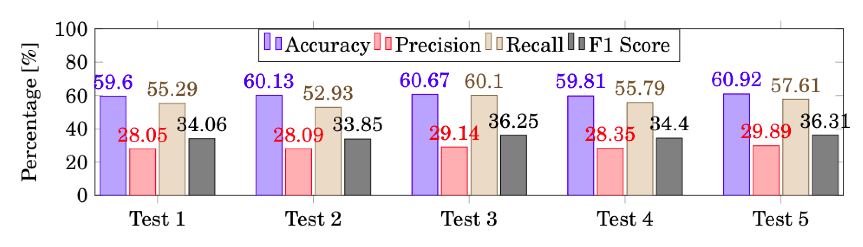
2.5.2. LSTM
2.5.3. DBMM
- is the normalization factor, necessary due to the continuous updating of the confidence level;
- is the probability distribution of transition between class variables over time;
- The weight is estimated through the level of confidence based on entropy;
- is the a posteriori result for the base classifier i in the instant of time t, which becomes the probability i of the mixing model, with being N the total number of classifiers considered in the model.
2.6. Evaluation Metrics
3. Experimental Results
3.1. Evaluating Features
3.2. Benchmark
3.3. Discussion
4. Conclusions and Future Work
Author Contributions
Acknowledgments
Conflicts of Interest
References
- Parasher, M.; Sharma, S.; Sharma, A.; Gupta, J. Anatomy on pattern recognition. Indian J. Comput. Sci. Eng. (IJCSE) 2011, 2, 371–378. [Google Scholar]
- Huang, Y.P.; Liu, Y.Y.; Hsu, W.H.; Lai, L.J.; Lee, M.S. Monitoring and Assessment of Rehabilitation Progress on Range of Motion After Total Knee Replacement by Sensor-Based System. Sensors 2020, 20, 1703. [Google Scholar]
- Sharma, P.; Kaur, M. Classification in pattern recognition: A review. Int. J. Adv. Res. Comput. Sci. Softw. Eng. 2013, 3, 298–306. [Google Scholar]
- Couceiro, M.S.; Dias, G.; Araújo, D.; Davids, K. The ARCANE project: How an ecological dynamics framework can enhance performance assessment and prediction in football. Sport. Med. 2016, 46, 1781–1786. [Google Scholar]
- Dicharry, J. Kinematics and kinetics of gait: From lab to clinic. Clin. Sport. Med. 2010, 29, 347–364. [Google Scholar]
- Brown, A.M.; Zifchock, R.A.; Hillstrom, H.J. The effects of limb dominance and fatigue on running biomechanics. Gait Posture 2014, 39, 915–919. [Google Scholar] [CrossRef]
- Mero, A.; Komi, P.; Gregor, R. Biomechanics of sprint running. Sport. Med. 1992, 13, 376–392. [Google Scholar] [CrossRef]
- Clermont, C.A.; Benson, L.C.; Osis, S.T.; Kobsar, D.; Ferber, R. Running patterns for male and female competitive and recreational runners based on accelerometer data. J. Sport. Sci. 2019, 37, 204–211. [Google Scholar]
- Yang, J.; Nguyen, M.N.; San, P.P.; Li, X.L.; Krishnaswamy, S. Deep convolutional neural networks on multichannel time series for human activity recognition. In Proceedings of the Twenty-Fourth International Joint Conference on Artificial Intelligence, Buenos Aires, Argentina, 25–31 July 2015. [Google Scholar]
- Zhu, S.; Xiao, Y.; Ma, W. Human Action Recognition Based on Multiple Features and Modified Deep Learning Model. Int. J. Pattern Recognit. Artif. Intell. 2020, 34, 2055022. [Google Scholar]
- Vital, J.P.; Faria, D.R.; Dias, G.; Couceiro, M.S.; Coutinho, F.; Ferreira, N.M. Combining discriminative spatiotemporal features for daily life activity recognition using wearable motion sensing suit. Pattern Anal. Appl. 2017, 20, 1179–1194. [Google Scholar] [CrossRef]
- Conforti, I.; Mileti, I.; Del Prete, Z.; Palermo, E. Measuring Biomechanical Risk in Lifting Load Tasks Through Wearable System and Machine-Learning Approach. Sensors 2020, 20, 1557. [Google Scholar] [CrossRef]
- Huang, Z.; Niu, Q.; Xiao, S. Human Behavior Recognition Based on Motion Data Analysis. Int. J. Pattern Recognit. Artif. Intell. 2019, 34, 2056005. [Google Scholar] [CrossRef]
- Ermes, M.; Pärkkä, J.; Mäntyjärvi, J.; Korhonen, I. Detection of daily activities and sports with wearable sensors in controlled and uncontrolled conditions. IEEE Trans. Inf. Technol. Biomed. 2008, 12, 20–26. [Google Scholar] [CrossRef]
- Walter, R.T. Worldwide Survey of Fitness Trends for 2019. Am. Coll. Sport. Med. Health Fit. J. 2018, 19, 9–18. [Google Scholar] [CrossRef]
- Papić, V.; Rogulj, N.; Pleština, V. Identification of sport talents using a web-oriented expert system with a fuzzy module. Expert Syst. Appl. 2009, 36, 8830–8838. [Google Scholar] [CrossRef]
- Rossi, A.; Pappalardo, L.; Cintia, P.; Iaia, F.M.; Fernàndez, J.; Medina, D. Effective injury forecasting in soccer with GPS training data and machine learning. PLoS ONE 2018, 13, e0201264. [Google Scholar] [CrossRef]
- Grunz, A.; Memmert, D.; Perl, J. Tactical pattern recognition in soccer games by means of special self-organizing maps. Hum. Mov. Sci. 2012, 31, 334–343. [Google Scholar] [CrossRef]
- Montoliu, R.; Martín-Félez, R.; Torres-Sospedra, J.; Martínez-Usó, A. Team activity recognition in Association Football using a Bag-of-Words-based method. Hum. Mov. Sci. 2015, 41, 165–178. [Google Scholar] [CrossRef]
- Del Boca, A.; Park, D.C. Myoelectric signal recognition using fuzzy clustering and artificial neural networks in real time. In Proceedings of the 1994 IEEE International Conference on Neural Networks (ICNN’94), Orlando, FL, USA, 28 June–2 July 1994; Volume 5, pp. 3098–3103. [Google Scholar]
- Al-Mulla, M.R.; Sepulveda, F. Novel feature modelling the prediction and detection of semg muscle fatigue towards an automated wearable system. Sensors 2010, 10, 4838–4854. [Google Scholar] [CrossRef]
- Faria, D.R.; Premebida, C.; Nunes, U. A probabilistic approach for human everyday activities recognition using body motion from RGB-D images. In Proceedings of the 23rd IEEE International Symposium on Robot and Human Interactive Communication, Edinburgh, UK, 25–29 August 2014; pp. 732–737. [Google Scholar]
- Hochreiter, S.; Schmidhuber, J. Long short-term memory. Neural Comput. 1997, 9, 1735–1780. [Google Scholar] [CrossRef]
- Bishop, C.M. Pattern Recognition and Machine Learning; Springer: Berlin/Heidelberg, Germany, 2006. [Google Scholar]
- Jain, A.K.; Mao, J.; Mohiuddin, K.M. Artificial neural networks: A tutorial. Computer 1996, 29, 31–44. [Google Scholar]
- Sak, H.; Senior, A.; Beaufays, F. Long short-term memory recurrent neural network architectures for large scale acoustic modeling. In Proceedings of the Fifteenth Annual Conference of the International Speech Communication Association, Singapore, 14–18 September 2014. [Google Scholar]
- Graves, A.; Schmidhuber, J. Framewise phoneme classification with bidirectional LSTM and other neural network architectures. Neural Netw. 2005, 18, 602–610. [Google Scholar] [CrossRef]
- Bouktif, S.; Fiaz, A.; Ouni, A.; Serhani, M.A. Optimal deep learning lstm model for electric load forecasting using feature selection and genetic algorithm: Comparison with machine learning approaches. Energies 2018, 11, 1636. [Google Scholar] [CrossRef]
- Arras, L.; Arjona-Medina, J.; Widrich, M.; Montavon, G.; Gillhofer, M.; Müller, K.R.; Hochreiter, S.; Samek, W. Explaining and interpreting LSTMs. In Explainable Ai: Interpreting, Explaining and Visualizing Deep Learning; Springer: Berlin/Heidelberg, Germany, 2019; pp. 211–238. [Google Scholar]
- Glorot, X.; Bengio, Y. Understanding the difficulty of training deep feedforward neural networks. In Proceedings of the Thirteenth International Conference on Artificial Intelligence and Statistics, Sardinia, Italy, 13–15 May 2010; pp. 249–256. [Google Scholar]
- Bramer, M. Ensemble classification. In Principles of Data Mining; Springer: Berlin/Heidelberg, Germany, 2013; pp. 209–220. [Google Scholar]
- Faria, D.R.; Vieira, M.; Premebida, C.; Nunes, U. Probabilistic human daily activity recognition towards robot-assisted living. In Proceedings of the 2015 24th IEEE International Symposium on Robot and Human Interactive Communication (RO-MAN), Kobe, Japan, 31 August–4 September 2015; pp. 582–587. [Google Scholar]
- Daniel, G. Principles of Artificial Neural Networks; World Scientific: Singapore, 2013; Volume 7. [Google Scholar]
- Sabeti, M.; Boostani, R.; Katebi, S.; Price, G. Selection of relevant features for EEG signal classification of schizophrenic patients. Biomed. Signal Process. Control. 2007, 2, 122–134. [Google Scholar] [CrossRef]


| Target Actions | ||||||
|---|---|---|---|---|---|---|
| Walking | Walking with ball | Running | Running with ball | shooting | Passing | Jumping |
| TraXports Example File | ||||
|---|---|---|---|---|
| idx | posX1 | posY1 | posW1 | ... |
| 1 | 0 | 0 | 100 | ... |
| MBody3 Example File | ||||||
|---|---|---|---|---|---|---|
| R.Quad | L.Quad | R.Hams | L.Hams | R.Gluteo | L.Gluteo | Time(s) |
| 45 | 35 | 21 | 2 | 11 | 3 | 0.04 |
| Actions | Number of Trials |
|---|---|
| Running | 183 |
| Running w/ball | 57 |
| Passing | 80 |
| Walking | 690 |
| Walking w/ball | 27 |
| shooting | 15 |
| Jumping | 24 |
| 70% of the Dataset. | |
| Actions | Number of Trials |
| Running | 128 |
| Running w/ball | 40 |
| Passing | 56 |
| Walking | 483 |
| Walking w/ball | 19 |
| shooting | 11 |
| Jumping | 17 |
| 30% of the Dataset. | |
| Actions | Number of Trials |
| Running | 55 |
| Running w/ball | 17 |
| Passing | 24 |
| Walking | 207 |
| Walking w/ball | 08 |
| shooting | 04 |
| Jumping | 07 |
| Target Class | Running | 6.38 ± 1.09 1.98% | 0.02 ± 0.03 0.01% | 0.01±0.01 0.001% | 48.58 ± 1.11 15.09% | 0.01 ± 0.01 0.003% | 0 ± 0 0% | 0.01 ± 0.01 0.002% |
| Running w/ball | 1.67 ± 0.15 0.52% | 0.10± 0.03 0.03% | 0 ± 0 0% | 15.22 ± 0.18 4.73% | 0.01± 0.01 0.001% | 0 ± 0 0% | 0.01 ± 0.01 0.002% | |
| Passing | 1.04 ± 0.22 0.32% | 0.04 ± 0.05 0.01% | 0.17 ± 0.08 0.05% | 22.79 ± 0.23 7.08% | 0.01 ±0.02 0.004% | 0 ± 0 0% | 0 ± 0 0% | |
| Walking | 4.37 ± 0.24 1.36% | 0.04 ± 0.03 0.01% | 0.02 ± 0.08 0.01% | 202.54 ± 0.29 62.90% | 0.02 ± 0.02 0.01% | 0 ± 0 0% | 0.01 ± 0.01 0.003% | |
| Walking w/ball | 0.23 ± 0.12 0.07% | 0 ± 0 0% | 0 ± 0 0% | 7.73 ± 0.16 2.40% | 0.04 ± 0.03 0.01% | 0 ± 0 0% | 0 ± 0 0% | |
| Shoting | 0.18 ± 0.12 0.06% | 0 ± 0 0% | 0 ± 0 0% | 3.81 ± 0.13 1.18% | 0 ± 0 0% | 0.01 ± 0.01 0.003% | 0 ± 0 0% | |
| Jumping | 0.10 ± 0.02 0.03% | 0.01 ± 0.01 0.003% | 0 ± 0 0% | 6.82 ± 0.06 2.12% | 0 ± 0 0% | 0 ± 0 0% | 0.07 ± 0.03 0.02% | |
| Running | Running w/ball | Passing | Walking | Walking w/ball | Shoting | Jumping | ||
| Output Class | ||||||||
| Actions | Accuracy | Precision | Recall | F1Score |
|---|---|---|---|---|
| Running | 82.73 ± 0.8253 | 11.60 ± 0.48 | 45.63 ± 0.55 | 18.50 ± 0.51 |
| Running w/ball | 94.72 ± 0.90 | 0.58 ± 0.09 | 49.10 ± 0.20 | 1.15 ± 0.12 |
| Passing | 92.58 ± 0.88 | 0.70 ± 0.13 | 86.03 ± 0.80 | 1.38 ± 0.22 |
| Walking | 66.02 ± 0.52 | 97.85 ± 0.48 | 65.87 ± 0.13 | 78.74 ± 0.21 |
| Walking w/ball | 97.51 ± 0.92 | 0.52 ± 0.10 | 45.07 ± 0.36 | 1.02 ± 0.16 |
| shooting | 98.76 ± 0.95 | 0.22 ± 0.05 | 100 ± 1 | 0.43 ± 0.09 |
| Jumping | 97.84 ± 0.97 | 0.99 ± 0.21 | 83.38 ± 0.57 | 1.95 ± 0.31 |
| Total | 90.03 ± 0.85 | 16.06 ± 0.22 | 67.87 ± 0.52 | 14.74 ± 0.23 |
| Target Class | Running | 11.07 ± 2.76 3.44% | 2.03 ± 1.43 0.63% | 1.80 ± 0.98 0.06% | 38.20 ± 3.15 11.86% | 0.57 ± 0.62 0.18% | 00.70 ± 0.82 0.22% | 0.63 ± 0.87 0.20% |
| Running w/ball | 3.07 ± 1.41 0.95% | 1.43 ± 1.05 0.45% | 0.60 ± 0.71 0.19% | 9.87 ± 1.84 3.06% | 0.43 ± 0.72 0.14% | 1.10 ± 1.11 0.34% | 0.50 ± 0.67 0.16% | |
| Passing | 2.43 ± 1.36 0.76% | 1.63 ± 1.35 0.51% | 10.93 ± 2.53 3.40% | 1.83 ± 1.75 0.57% | 1.73 ± 1.36 0.54% | 3.40 ± 1.40 1.06% | 2.03 ± 1.11 0.63% | |
| Walking | 18.17 ± 3.85 5.64% | 2.40 ± 1.70 0.75% | 1.60 ± 1.17 0.50% | 182.20 ± 4.97 56.58% | 1.00 ± 1.21 0.31% | 0.83 ± 0.97 0.26% | 0.80 ± 0.79 0.25% | |
| Walking w/ball | 0.73 ± 0.93 0.23% | 0.33 ± 0.47 0.10% | 0.57 ± 0.72 1.18% | 5.77 ± 1.05 1.79% | 0.03 ± 0.18 0.01% | 0.43 ± 0.50 0.14% | 0.13 ± 0.34 0.04% | |
| Shoting | 0.43 ± 0.50 0.14% | 0.83 ± 0.86 0.26% | 1.40 ± 0.84 0.44% | 0.33 ± 0.65 1.10% | 0.17 ± 0.37 0.05% | 0.50 ± 0.56 0.16% | 0.33 ± 0.47 0.10% | |
| Jumping | 0.77 ± 0.80 0.24% | 0.80 ± 0.83 0.25% | 1.60 ± 1.11 0.50% | 1.67 ± 1.11 0.52% | 0.33 ± 0.60 0.10% | 0.83 ± 0.90 0.26% | 1.00 ± 0.77 0.31% | |
| Running | Running w/ball | Passing | Walking | Walking w/ball | Shoting | Jumping | ||
| Output Class | ||||||||
| Actions | Accuracy | Precision | Recall | F1Score |
|---|---|---|---|---|
| Running | 57.45 ± 0.38 | 30.30 ± 0.62 | 65.62 ± 0.59 | 41.31 ± 0.67 |
| Running w/ball | 55.07 ± 0.29 | 15.11 ± 0.56 | 58.91 ± 3.67 | 23.41 ± 1.12 |
| Passing | 77.28 ± 0.27 | 58.86 ± 0.37 | 93.01 ± 0.32 | 71.89± 0.41 |
| Walking | 72.99 ± 0.22 | 76.00 ± 0.11 | 71.78 ± 0.34 | 73.80± 0.13 |
| Walking w/ball | 50.61 ± 0.34 | — | 2.88 ± 0.53 | 0.82± 0.15 |
| shooting | 53.42 ± 0.74 | 7.95 ± 1.45 | 43.30 ± 7.90 | 12.56 ± 2.29 |
| Jumping | 59.59 ± 2.70 | 21.01 ± 5.28 | 67.74 ± 5.44 | 30.38 ± 6.52 |
| Total | 60.92 ± 0.70 | 29.89 ± 1.20 | 57.61 ± 2.68 | 36.31 ± 1.61 |
| Target Class | Running | 44.42 ± 0.69 13.79% | 0.90 ± 0.18 0.28% | 0.57±0.13 0.18% | 8.64 ± 0.67 2.68% | 0.23 ± 0.11 0.07% | 0.11 ± 0.07 0.03% | 0.13 ± 0.09 0.04% |
| Running w/ball | 1.11 ± 0.81 0.34% | 12.28± 1.34 3.81% | 0.28 ± 0.31 0.09% | 3.12 ± 1.06 0.97% | 0.09 ± 0.22 0.03% | 0.09 ± 0.18 0.03% | 0.04 ± 0.12 0.01% | |
| Passing | 1.44 ± 0.94 0.44% | 0.63 ± 0.67 0.20% | 15.98 ± 2.11 4.96% | 5.60 ± 1.68 1.74% | 0.24 ±0.25 0.07% | 0.03 ± 0.10 0.01% | 0.09 ± 0.16 0.03% | |
| Walking | 6.99 ± 0.12 2.17% | 2.22 ± 0.07 0.69% | 1.55 ± 0.08 0.48% | 194.70 ± 0.18 60.47% | 0.76 ± 0.04 0.24% | 0.33 ± 0.03 0.10% | 0.46 ± 0.04 0.14% | |
| Walking w/ball | 0.19 ± 0.79 0.06% | 0.08 ± 0.43 0.02% | 0.08 ± 0.36 0.03% | 0.84 ± 0.97 0.26% | 6.79 ± 1.15 2.11% | 0.01 ± 0.08 0.002% | 0.01 ± 0.18 0.004% | |
| Shoting | 0.27 ± 1.28 0.08% | 0.15 ± 1.17 0.05% | 0.04 ± 0.68 0.01% | 0.84 ± 0.97 0.26% | 0.01 ± 0.58 0.005% | 2.67 ± 3.89 0.83% | 0.02 ± 0.56 0.01% | |
| Jumping | 0.23 ± 1.09 0.07% | 0.04 ± 0.41 0.01% | 0.07 ± 0.62 0.02% | 1.11 ± 2.18 0.34% | 0.04 ± 0.40 0.01% | 0.002 ± 0 0.001% | 5.51 ± 2.73 1.71% | |
| Running | Running w/ball | Passing | Walking | Walking w/ball | Shoting | Jumping | ||
| Output Class | ||||||||
| Actions | Accuracy | Precision | Recall | F1Score |
|---|---|---|---|---|
| Running | 93.54 ± 0.82 | 80.18 ± 0.36 | 81.18 ± 0.12 | 80.97 ± 0.18 |
| Running w/ball | 97.28 ± 0.09 | 72.21 ± 0.20 | 75.35 ± 0.04 | 73.75 ± 0.07 |
| Passing | 96.71 ± 0.83 | 66.56 ± 0.16 | 86.00 ± 0.03 | 75.04 ± 0.05 |
| Walking | 89.91 ± 0.71 | 94.06 ± 0.22 | 90.56 ± 0.07 | 92.28 ± 0.10 |
| Walking w/ball | 99.20 ± 0.88 | 84.82 ± 0.20 | 83.39 ± 0.04 | 84.10 ± 0.07 |
| shooting | 99.36 ± 0.77 | 66.75 ± 0.11 | 84.16 ± 0.02 | 74.45 ± 0.03 |
| Jumping | 99.29 ± 0.84 | 78.75 ± 0.15 | 88.22 ± 0.02 | 83.22 ± 0.04 |
| Total | 96.47 ± 0.71 | 77.70 ± 0.20 | 84.12 ± 0.05 | 80.54 ± 0.08 |
| Approaches | Train [s] | Test [s] |
|---|---|---|
| LSTM | 382.515 | 0.236 |
| DBMM | 29.397 | 0.382 |
| Algorithm | Accuracy | Precision | Recall | F1Score |
|---|---|---|---|---|
| ANN | 90.03 ± 0.85 | 16.06 ± 0.22 | 67.87 ± 0.52 | 14.74 ± 0.23 |
| LSTM | 60.92 ± 0.70 | 29.89 ± 1.20 | 57.61 ± 2.68 | 36.31 ± 1.61 |
| DBMM | 96.47 ± 0.71 | 77.70 ± 0.20 | 84.12 ± 0.05 | 80.54 ± 0.08 |
| Total | 96.47 ± 0.71 | 77.70 ± 0.20 | 84.12 ± 0.05 | 80.54 ± 0.08 |
© 2020 by the authors. Licensee MDPI, Basel, Switzerland. This article is an open access article distributed under the terms and conditions of the Creative Commons Attribution (CC BY) license (http://creativecommons.org/licenses/by/4.0/).
Share and Cite
Rodrigues, A.C.N.; Pereira, A.S.; Mendes, R.M.S.; Araújo, A.G.; Couceiro, M.S.; Figueiredo, A.J. Using Artificial Intelligence for Pattern Recognition in a Sports Context. Sensors 2020, 20, 3040. https://doi.org/10.3390/s20113040
Rodrigues ACN, Pereira AS, Mendes RMS, Araújo AG, Couceiro MS, Figueiredo AJ. Using Artificial Intelligence for Pattern Recognition in a Sports Context. Sensors. 2020; 20(11):3040. https://doi.org/10.3390/s20113040
Chicago/Turabian StyleRodrigues, Ana Cristina Nunes, Alexandre Santos Pereira, Rui Manuel Sousa Mendes, André Gonçalves Araújo, Micael Santos Couceiro, and António José Figueiredo. 2020. "Using Artificial Intelligence for Pattern Recognition in a Sports Context" Sensors 20, no. 11: 3040. https://doi.org/10.3390/s20113040
APA StyleRodrigues, A. C. N., Pereira, A. S., Mendes, R. M. S., Araújo, A. G., Couceiro, M. S., & Figueiredo, A. J. (2020). Using Artificial Intelligence for Pattern Recognition in a Sports Context. Sensors, 20(11), 3040. https://doi.org/10.3390/s20113040