A Comparison of Different Counting Methods for a Holographic Particle Counter: Designs, Validations and Results


Abstract
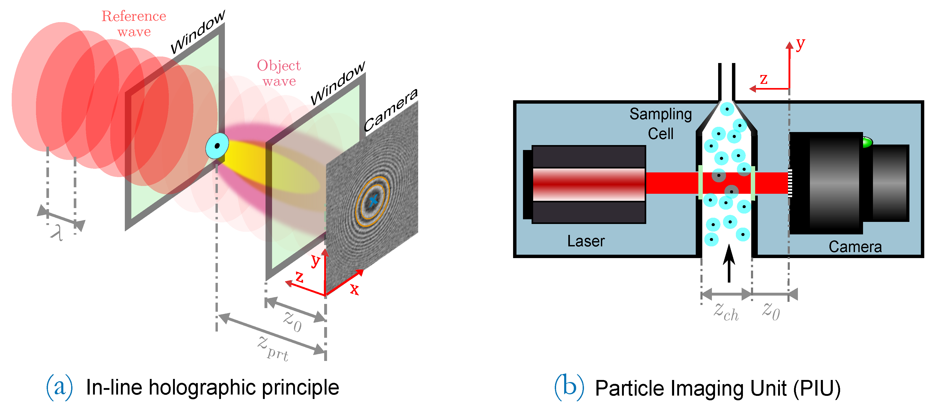
:1. Introduction
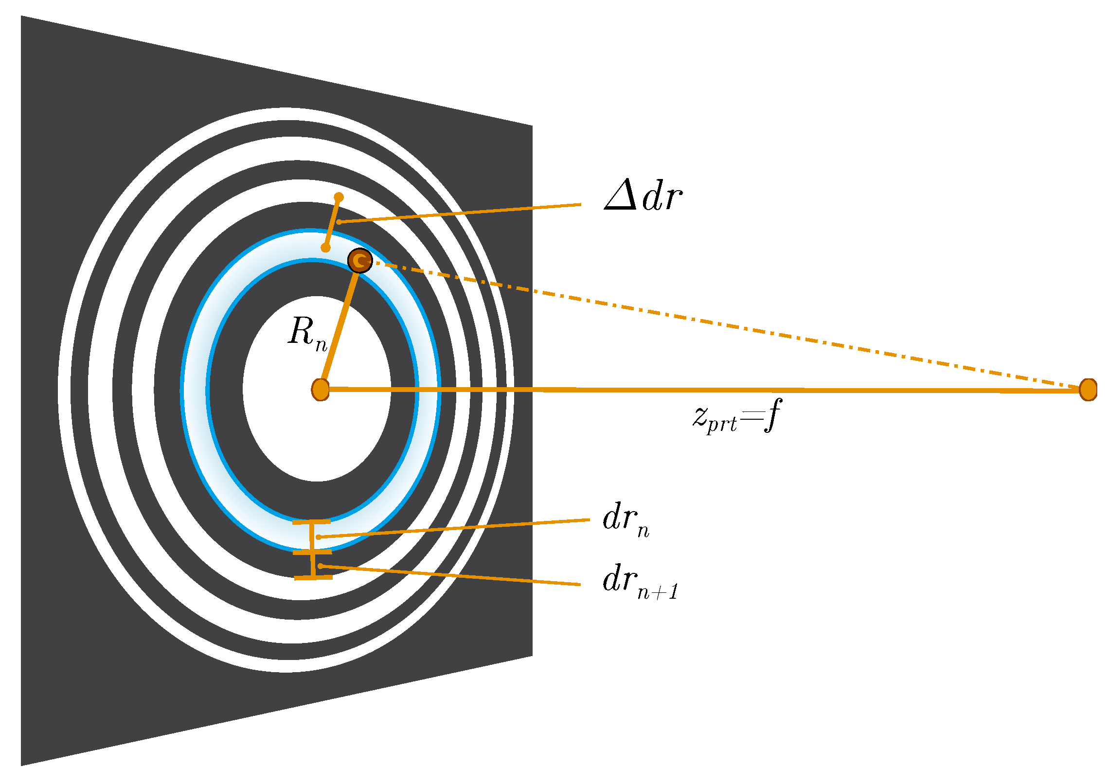
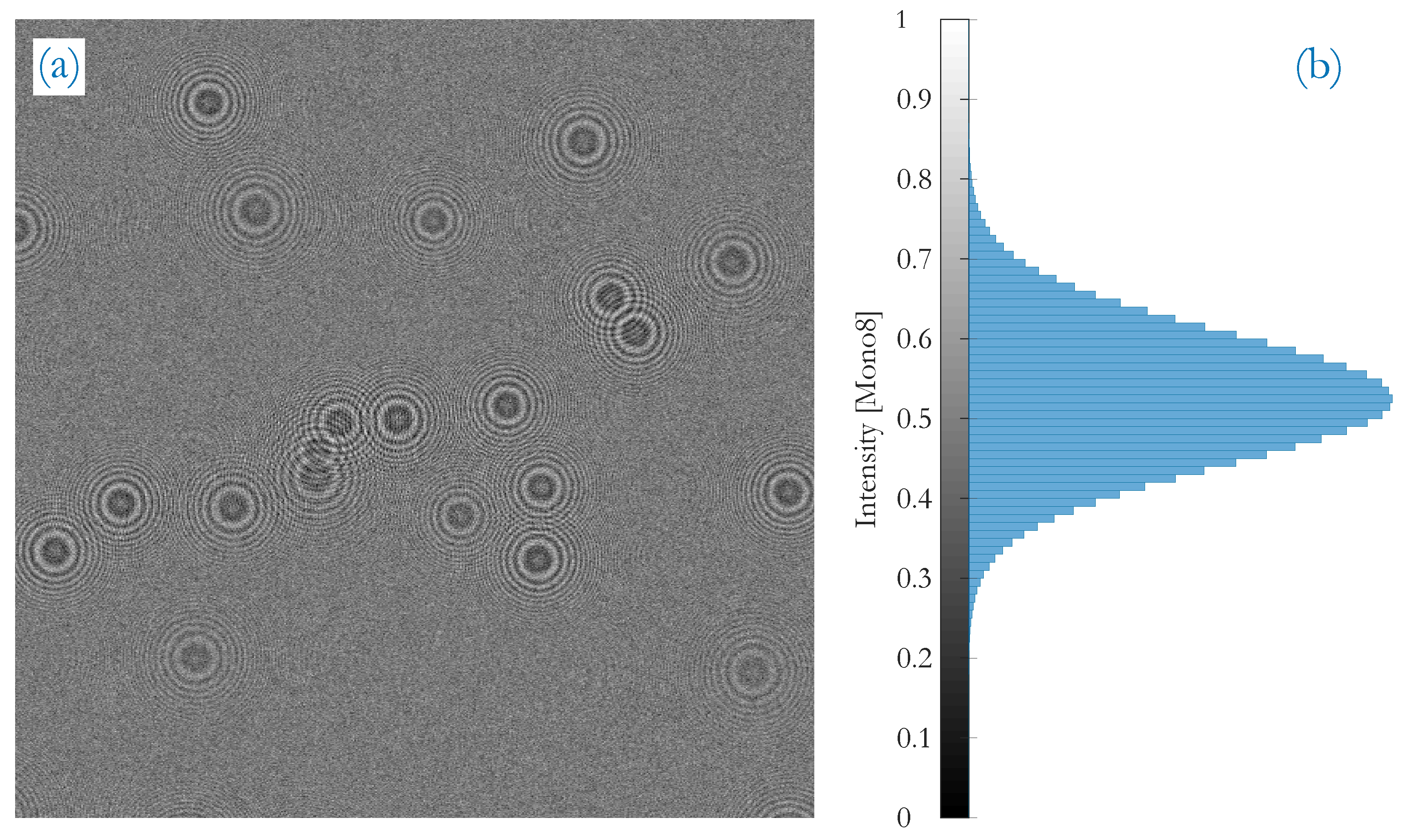
2. Fringe Patterns and Its Features
2.1. Information Content of Fringe Patterns
2.2. Features to Extract
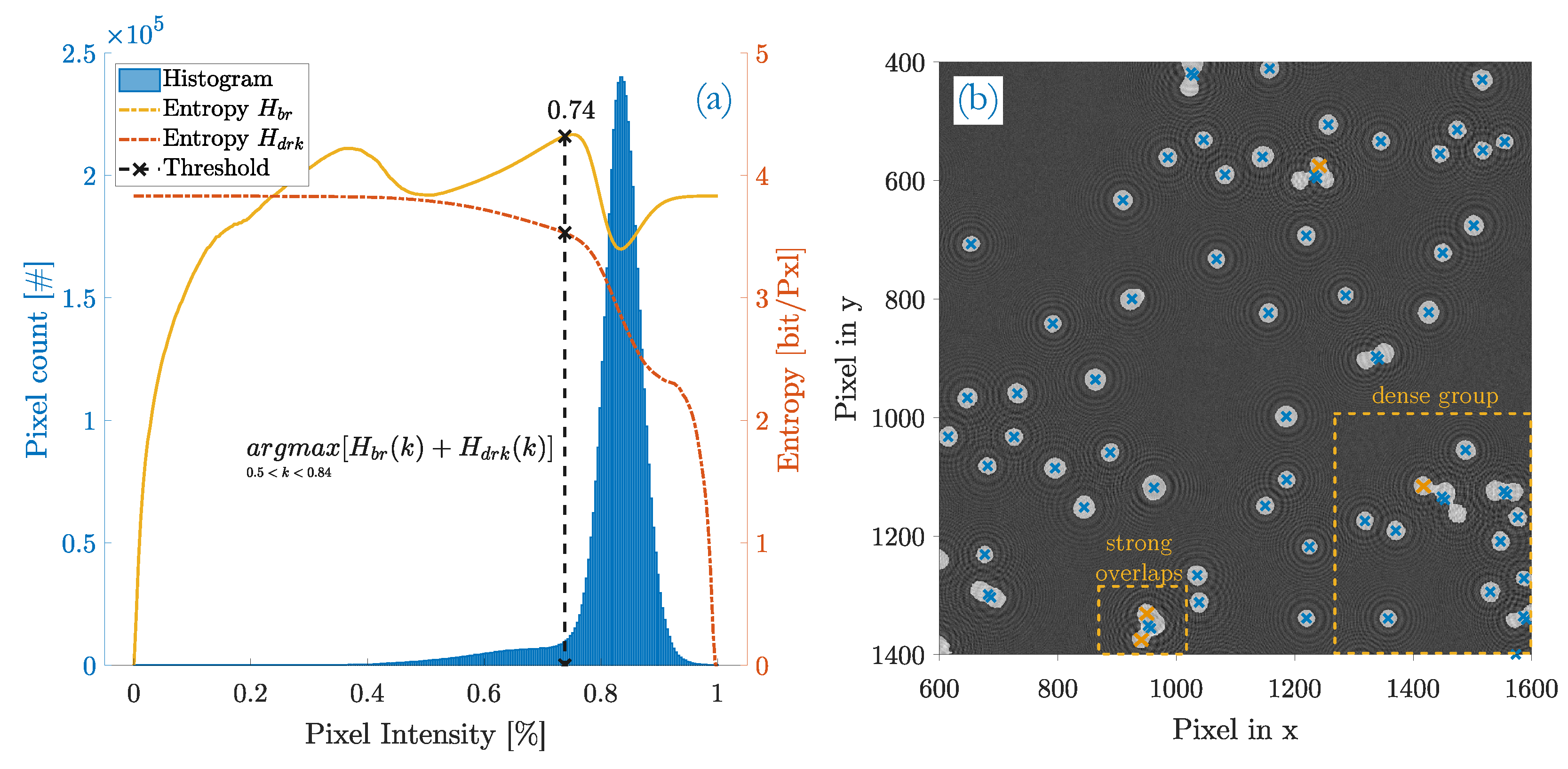
2.3. Intensity Dependence of Fringe Patterns
3. Methods
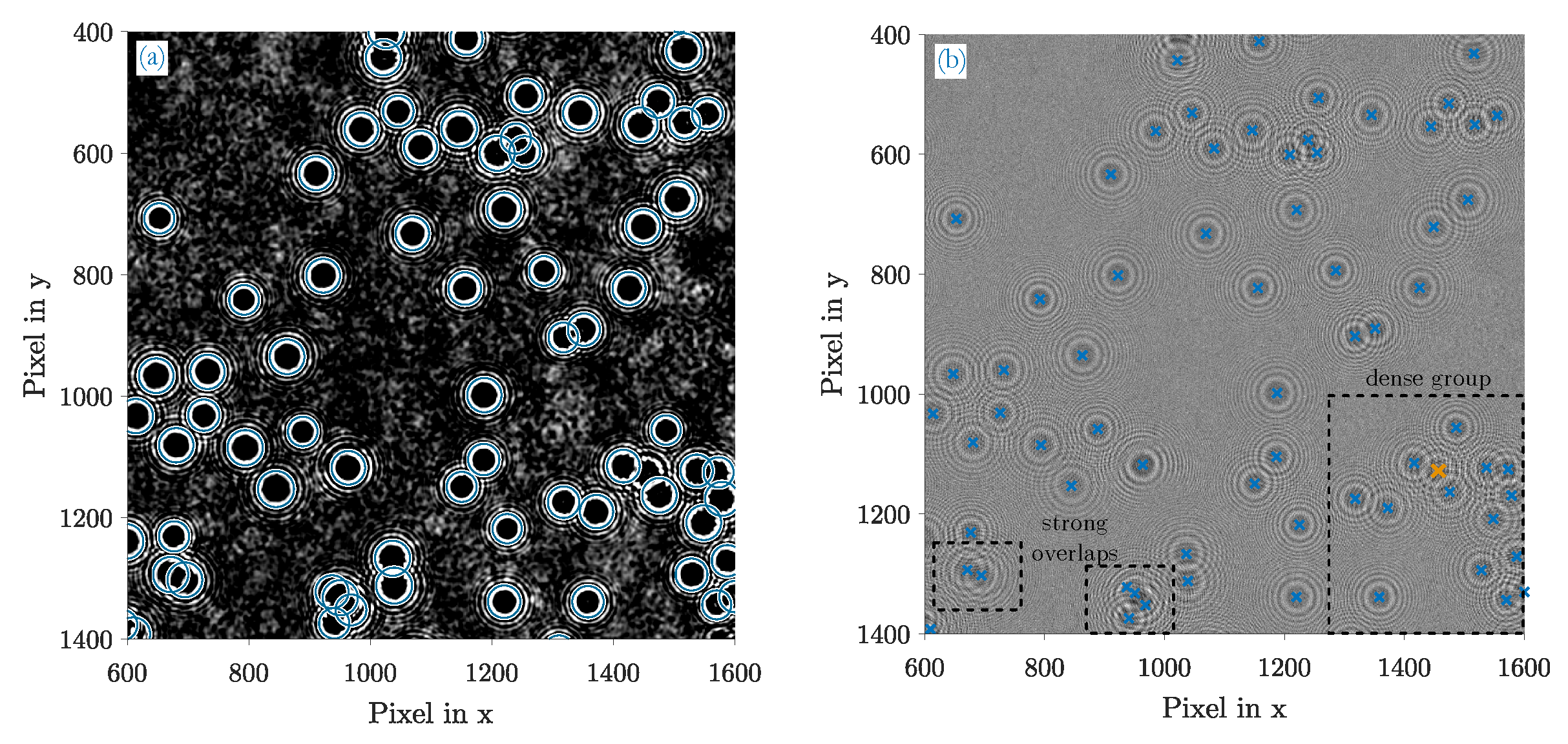
3.1. Customized Hough Transform
3.1.1. Working Principle
3.1.2. Image Preprocessing
3.1.3. Parameterization
3.2. Blob Detection
3.2.1. Blob Extraction Using Template Matching
3.2.2. Blob Segmentation
3.2.3. Blob Labeling and Counting
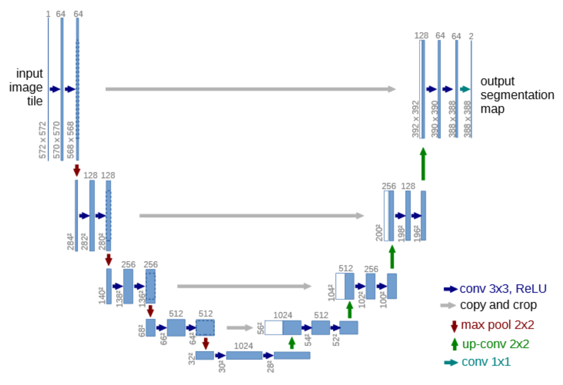
3.3. Deep Convolutional Neural Network (DCNN)
3.3.1. Working Principle
3.3.2. Training
3.3.3. Data Processing and Evaluation
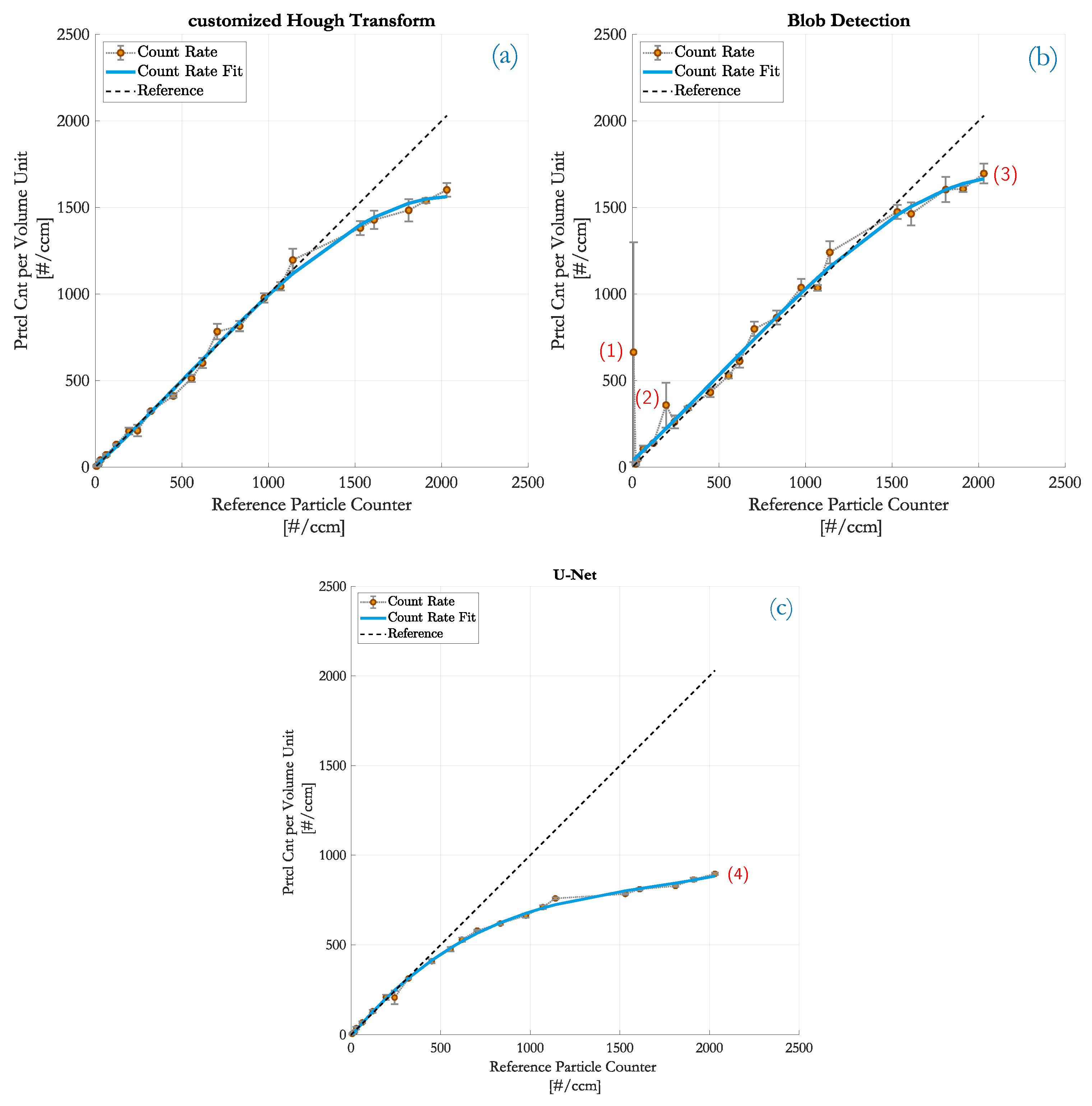
4. Results
4.1. Customized HT
4.2. Blob Detection
4.3. DCNN
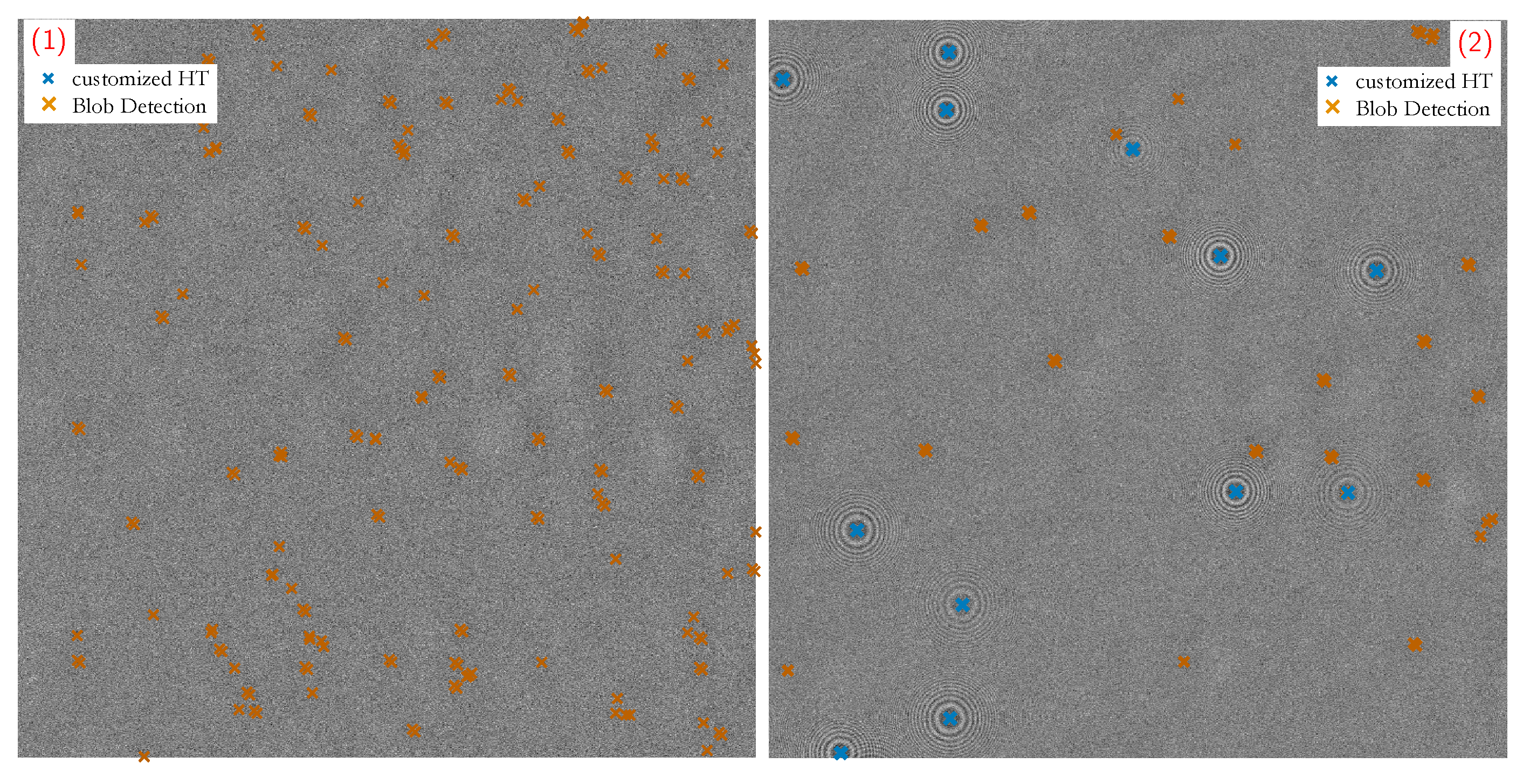
4.4. Comparison of Detection Performance
4.4.1. Details on Customized HT
4.4.2. Details on Blob Detection
4.4.3. Details on DCNN
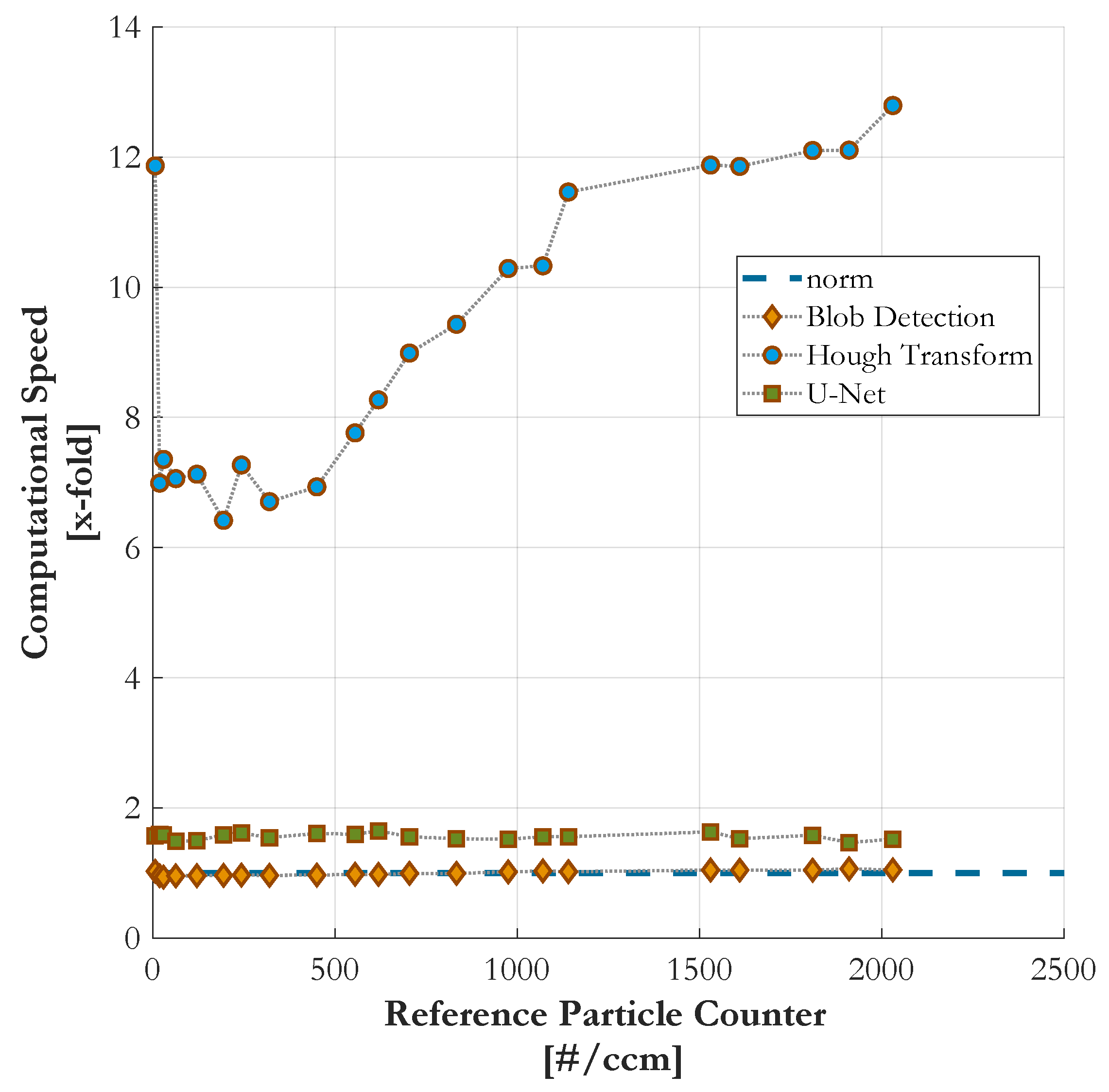
4.5. Comparison of Computational Speed
5. Conclusions
Author Contributions
Funding
Acknowledgments
Conflicts of Interest
Abbreviations
| CPC | Condensation Particle Counter |
| PC | Particle Counter |
| HPC | Holographic Particle Counter |
| HPCs | Holographic Particle Counters |
| CNM | Condensation Nucleus Magnifier |
| OPCs | Optical Particle Counters |
| PN | Particle Number |
| HPIV | Holography Particle Image Velocimetry |
| HT | Hough Transform |
| CHT | Circular Hough Transform |
| PIU | Particle Imaging Unit |
| APM | Aerosol Particle Model |
| ASM | Angular Spectrum Method |
| FZP | Fresnel Zone Plate |
| FZPs | Fresnel Zone Plates |
| DIH | Digital Inline Holography |
| 3D | Three-Dimensional |
| 2D | Two-Dimensional |
| SNR | Signal to Noise Ratio |
| DNN | Deep Neural Network |
| DCNN | Deep Convolutional Neural Network |
| LoG | Laplacian of Gaussian |
| DoF | Depth of Field |
| ReLu | Rectified Linear Unit |
| AI | Artificial Intelligence |
| RT | Real-Time |
| GPU | Graphics Processing Unit |
References
- Brunnhofer, G.; Bergmann, A.; Klug, A.; Kraft, M. Design & Validation of a Holographic Particle Counter. Sensors 2019, 19, 4899. [Google Scholar] [CrossRef] [Green Version]
- Pan, G.; Meng, H. Digital In-line Holographic PIV for 3D Particulate Flow Diagnostics. In Proceedings of the 4th International Symposium on Particle Image Velocimetry, Gottingen, Germany, 17–19 September 2001; pp. 611–617. [Google Scholar]
- Gire, J.; Denis, L.; Fournier, C.; Thiébaut, E.; Soulez, F.; Ducottet, C. Digital holography of particles: Benefits of the ‘inverse problem’ approach. Meas. Sci. Technol. 2008, 19, 074005. [Google Scholar] [CrossRef] [Green Version]
- Berg, M.J.; Heinson, Y.W.; Kemppinen, O.; Holler, S. Solving the inverse problem for coarse-mode aerosol particle morphology with digital holography. Sci. Rep. 2017, 7, 1–9. [Google Scholar] [CrossRef] [PubMed] [Green Version]
- Murata, S.; Yasuda, N. Potential of digital holography in particle measurement. Opt. Laser Technol. 2001, 32, 567–574. [Google Scholar]
- Malek, M.; Allano, D.; Coëtmellec, S.; Özkul, C.; Lebrun, D. Digital in-line holography for three-dimensional-two-components particle tracking velocimetry. Meas. Sci. Technol. 2004, 15, 699–705. [Google Scholar] [CrossRef]
- Poon, T.C.; Liu, J.P. Introduction to Modern Digital Holography; Cambridge University Press: Cambridge, UK, 2014; p. 223. [Google Scholar]
- Gonzalez, R.; Woods, R. Digital Image Processing; Prentice Hall: Upper Saddle River, NJ, USA, 2002; p. 190. [Google Scholar] [CrossRef]
- Brunnhofer, G.; Bergmann, A. Modelling a Holographic Particle Counter. Proceedings 2018, 2, 967. [Google Scholar] [CrossRef] [Green Version]
- Attwood, D.; Sakdinawat, A. X-Rays and Extreme Ultraviolet Radiation: Principles and Applications, 2nd ed.; Cambridge University Press: Cambridge, UK, 2017. [Google Scholar] [CrossRef] [Green Version]
- Dixon, L.; Cheong, F.C.; Grier, D.G. Holographic particle-streak velocimetry. Opt. Express 2011, 19, 4393–4398. [Google Scholar] [CrossRef]
- Duda, R.O.; Hart, P.E. Use of the Hough transformation to detect lines and curves in pictures. Commun. ACM 1972, 15, 11–15. [Google Scholar] [CrossRef]
- Atherton, T.J.; Kerbyson, D.J. Using phase to represent radius in the coherent circle Hough transform. In IEE Colloquium on Hough Transforms; IET: London, UK, 1993; pp. 1–4. [Google Scholar]
- Atherton, T.; Kerbyson, D. Size invariant circle detection. Image Vis. Comput. 1999, 17, 795–803. [Google Scholar] [CrossRef]
- Kong, H.; Akakin, H.C.; Sarma, S.E. A generalized laplacian of gaussian filter for blob detection and its applications. IEEE Trans. Cybern. 2013, 43, 1719–1733. [Google Scholar] [CrossRef] [PubMed]
- Last, A. Fresnel Zone Plates 2016. Available online: http://www.x-ray-optics.de/index.php/en/types-of-optics/diffracting-optics/fresnel-zone-plates (accessed on 11 December 2019).
- Lindeberg, T. Detecting salient blob-like image structures and their scales with a scale-space primal sketch: A method for focus-of-attention. Int. J. Comput. Vis. 1993, 11, 283–318. [Google Scholar] [CrossRef] [Green Version]
- Jayanthi, N.; Indu, S. Comparison of image matching techniques. Int. J. Latest Trends Eng. Technol. 2016, 7, 396–401. [Google Scholar] [CrossRef]
- Kaspers, A. Blob Detection. Master’s Thesis, UMC Utrecht, Utrecht, The Netherlands, 2009. Available online: https://dspace.library.uu.nl/handle/1874/204781 (accessed on 11 December 2019).
- Sonka, M.; Hlavac, V.; Boyle, R. Image Processing, Analysis, and Machine Vision; Cengage Learning: Boston, MA, USA, 2014. [Google Scholar]
- Kittler, J.; Illingworth, J. On threshold selection using clustering criteria. EEE Trans. Syst. Man, Cybern. 1985, SMC-15, 652–655. [Google Scholar] [CrossRef]
- Lee, H.; Park, R. Comments on An optimal multiple threshold scheme for image segmentation. IEEE Trans. Syst. Man Cybern. 1990, 20, 741–742. [Google Scholar] [CrossRef]
- Kapur, J.N.; Sahoo, P.K.; Wong, A.K.C. A new method for gray-level picture thresholding using the entropy of the histogram. Comput. Vision Graph. Image Process. 1985, 29, 273–285. [Google Scholar] [CrossRef]
- Sezgin, M.; Sankur, B. Survey over image thresholding techniques and quantitative performance evaluation. J. Electron. Imaging 2004, 13, 146–165. [Google Scholar]
- Haralick, R.M.; Shapiro, L.G. Image segmentation techniques. Comput. Vision Graph. Image Process. 1985, 29, 100–132. [Google Scholar] [CrossRef]
- Girshick, R.; Donahue, J.; Darrell, T.; Malik, J. Rich feature hierarchies for accurate object detection and semantic segmentation. In Proceedings of the IEEE Conference on Computer Vision and Pattern Recognition, Washington, DC, USA, 23–28 June 2014; pp. 580–587. [Google Scholar]
- LeCun, Y.; Boser, B.; Denker, J.S.; Henderson, D.; Howard, R.E.; Hubbard, W.; Jackel, L.D. Backpropagation applied to handwritten zip code recognition. Neural Comput. 1989, 1, 541–551. [Google Scholar] [CrossRef]
- Krizhevsky, A.; Sutskever, I.; Hinton, G.E. Imagenet classification with deep convolutional neural networks. Adv. Neural Inf. Process. Syst. 2012, 25, 1097–1105. [Google Scholar] [CrossRef]
- Simonyan, K.; Zisserman, A. Two-stream convolutional networks for action recognition in videos. In Proceedings of the Advances in Neural Information Processing Systems, Montreal, QC, Canada, 8–13 December 2014; pp. 568–576. [Google Scholar]
- Ronneberger, O.; Fischer, P.; Brox, T. U-net: Convolutional networks for biomedical image segmentation. In Proceedings of the International Conference on Medical Image Computing and Computer-Assisted Intervention, Munich, Germany, 5–9 October 2015; Springer: Berlin/Heidelberg, Germany, 2015; pp. 234–241. [Google Scholar]
- Jia, Y.; Shelhamer, E.; Donahue, J.; Karayev, S.; Long, J.; Girshick, R.; Guadarrama, S.; Darrell, T. Caffe: Convolutional architecture for fast feature embedding. In Proceedings of the 22nd ACM international conference on Multimedia, Orlando, FL, USA, 3–7 November 2014; pp. 675–678. [Google Scholar]
- Em Segmentation Challenge. 2012. Available online: https://imagej.net/2011-10-25_-_EM_segmentation_challenge_(ISBI_-_2012) (accessed on 31 March 2020).
- TSI Incorporated. Model 3775 Condensation Particle Counter; Operation and Service Manual; TSI Incorporated: Shoreview, MN, USA, 2007. [Google Scholar]


| Number of Particles | Precision | Accuracy |
|---|---|---|
| 53 | 0.55 | 0.98 |
| 88 | 0.45 | 0.91 |
| 103 | 0.36 | 0.87 |
| 155 | 0.35 | 0.74 |
| 180 | 0.25 | 0.69 |
© 2020 by the authors. Licensee MDPI, Basel, Switzerland. This article is an open access article distributed under the terms and conditions of the Creative Commons Attribution (CC BY) license (http://creativecommons.org/licenses/by/4.0/).
Share and Cite
Brunnhofer, G.; Hinterleitner, I.; Bergmann, A.; Kraft, M. A Comparison of Different Counting Methods for a Holographic Particle Counter: Designs, Validations and Results. Sensors 2020, 20, 3006. https://doi.org/10.3390/s20103006
Brunnhofer G, Hinterleitner I, Bergmann A, Kraft M. A Comparison of Different Counting Methods for a Holographic Particle Counter: Designs, Validations and Results. Sensors. 2020; 20(10):3006. https://doi.org/10.3390/s20103006
Chicago/Turabian StyleBrunnhofer, Georg, Isabella Hinterleitner, Alexander Bergmann, and Martin Kraft. 2020. "A Comparison of Different Counting Methods for a Holographic Particle Counter: Designs, Validations and Results" Sensors 20, no. 10: 3006. https://doi.org/10.3390/s20103006
APA StyleBrunnhofer, G., Hinterleitner, I., Bergmann, A., & Kraft, M. (2020). A Comparison of Different Counting Methods for a Holographic Particle Counter: Designs, Validations and Results. Sensors, 20(10), 3006. https://doi.org/10.3390/s20103006