Geometric Model and Calibration Method for a Solid-State LiDAR


Abstract
1. Introduction
2. Problem and Model Formulation
2.1. The Problem
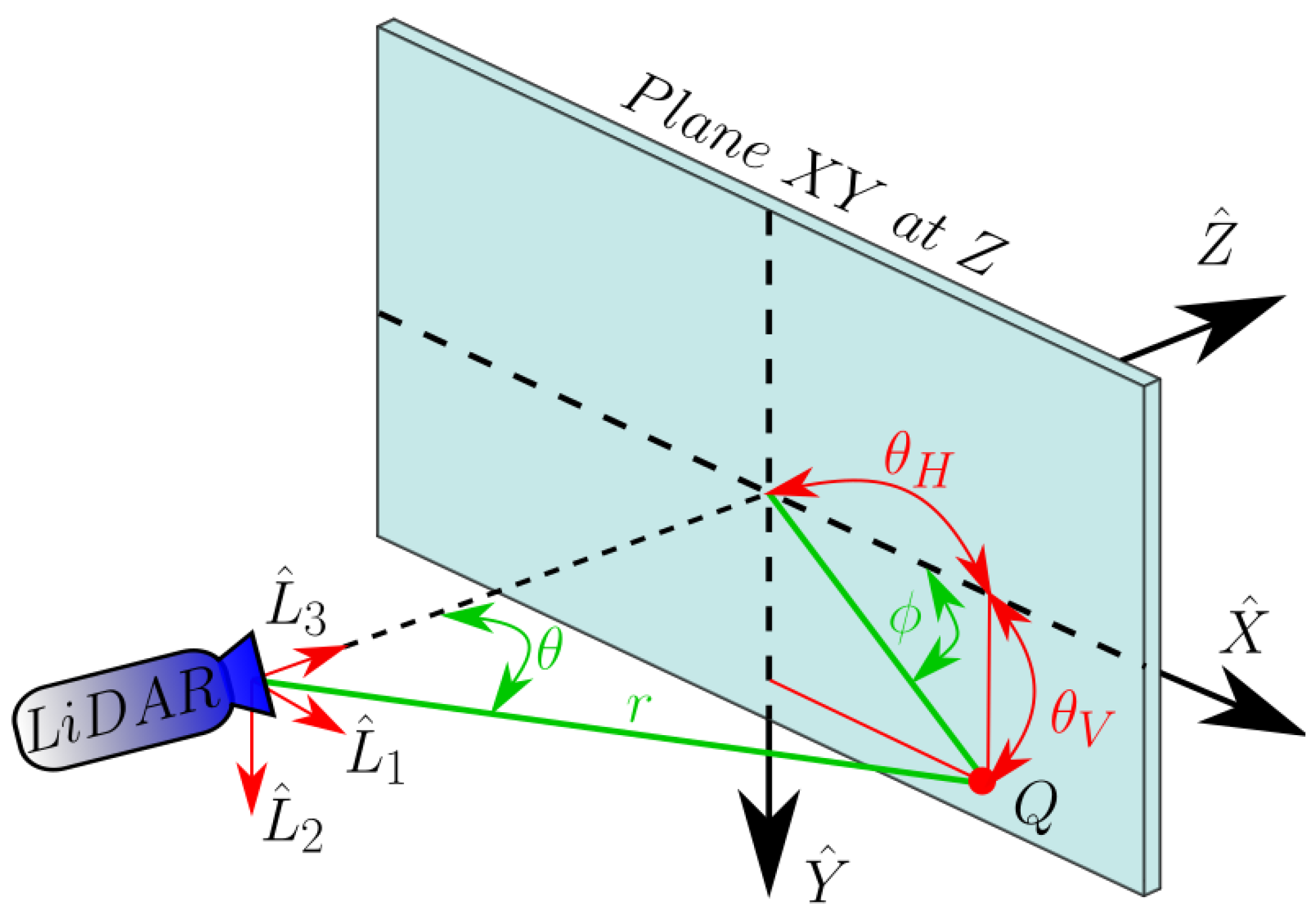
2.2. The Model
3. Materials and Methods
3.1. Calibration Method
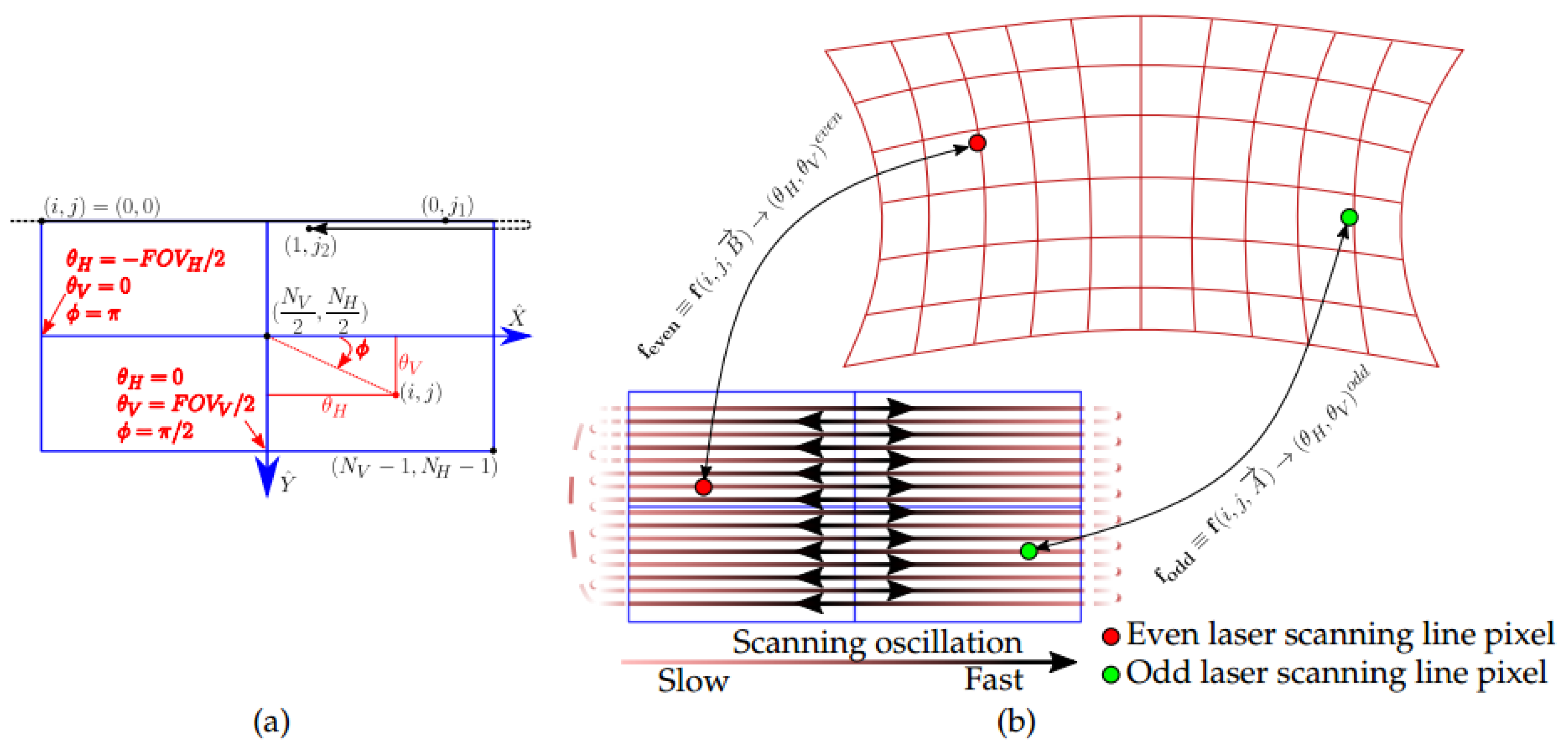
3.2. Distortion Mapping Equations
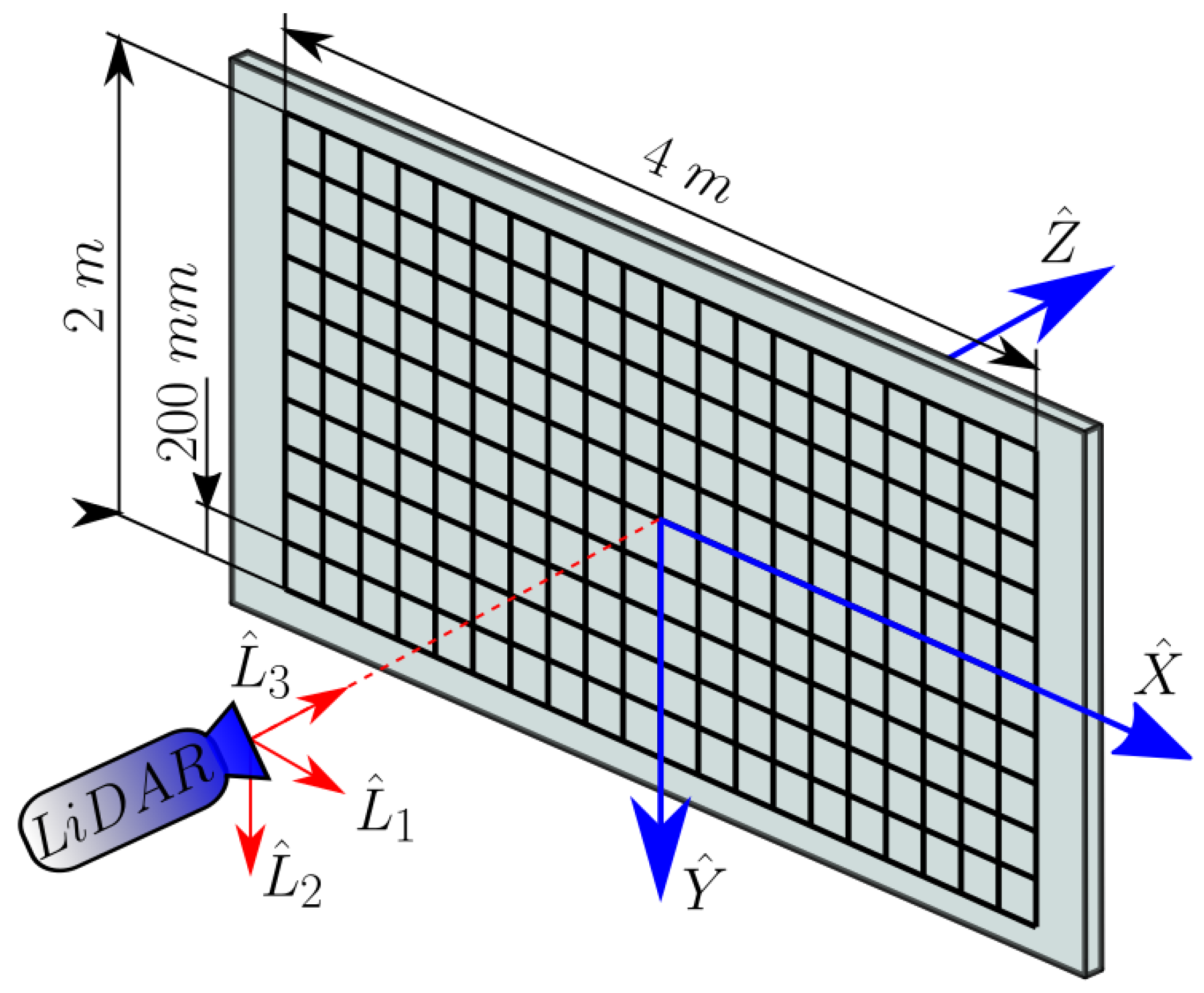
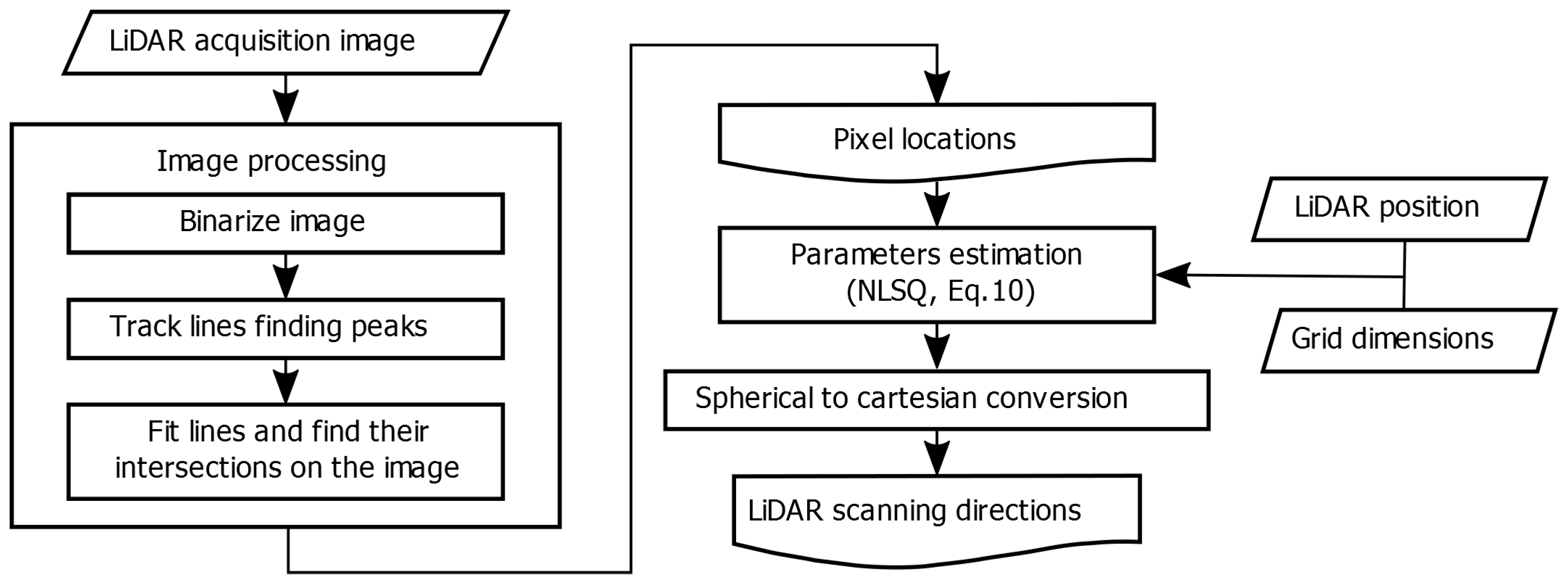
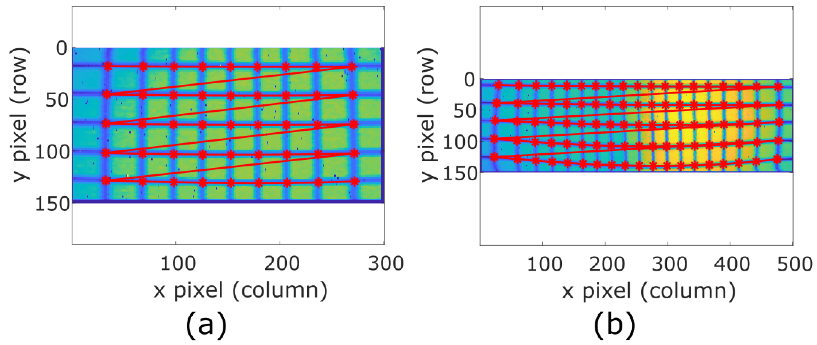
3.3. Calibration Pattern and Algorithm
| Algorithm 1: Image processing for obtaining the pixel locations of the lines’ intersections. |
 |
3.4. Prototypes
4. Results
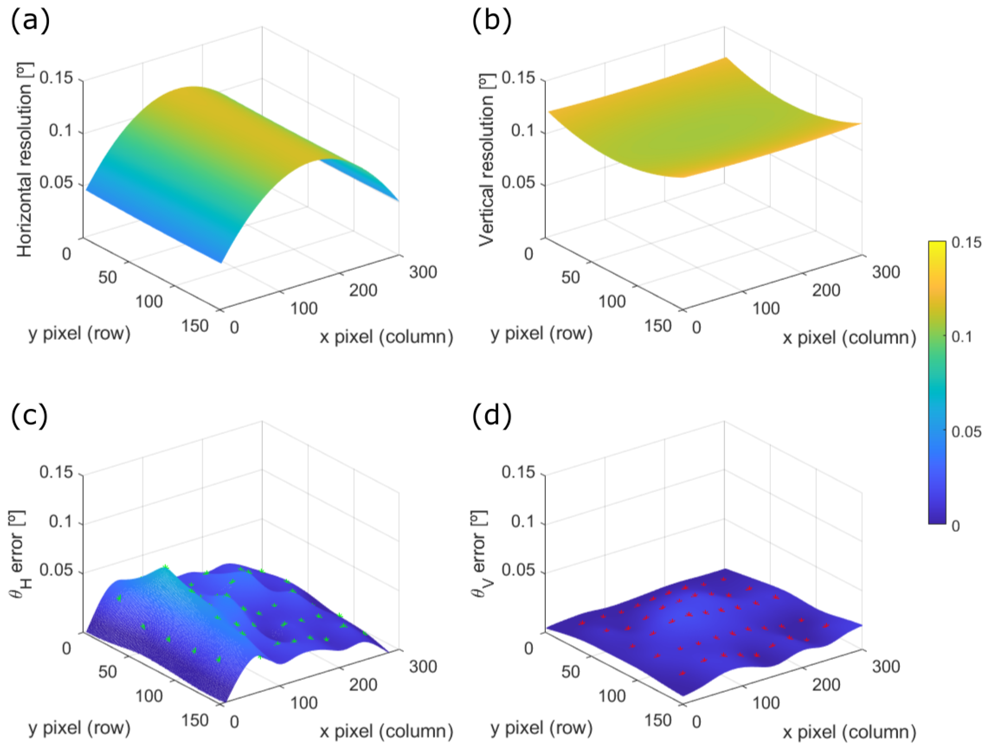
4.1. Model Simulation
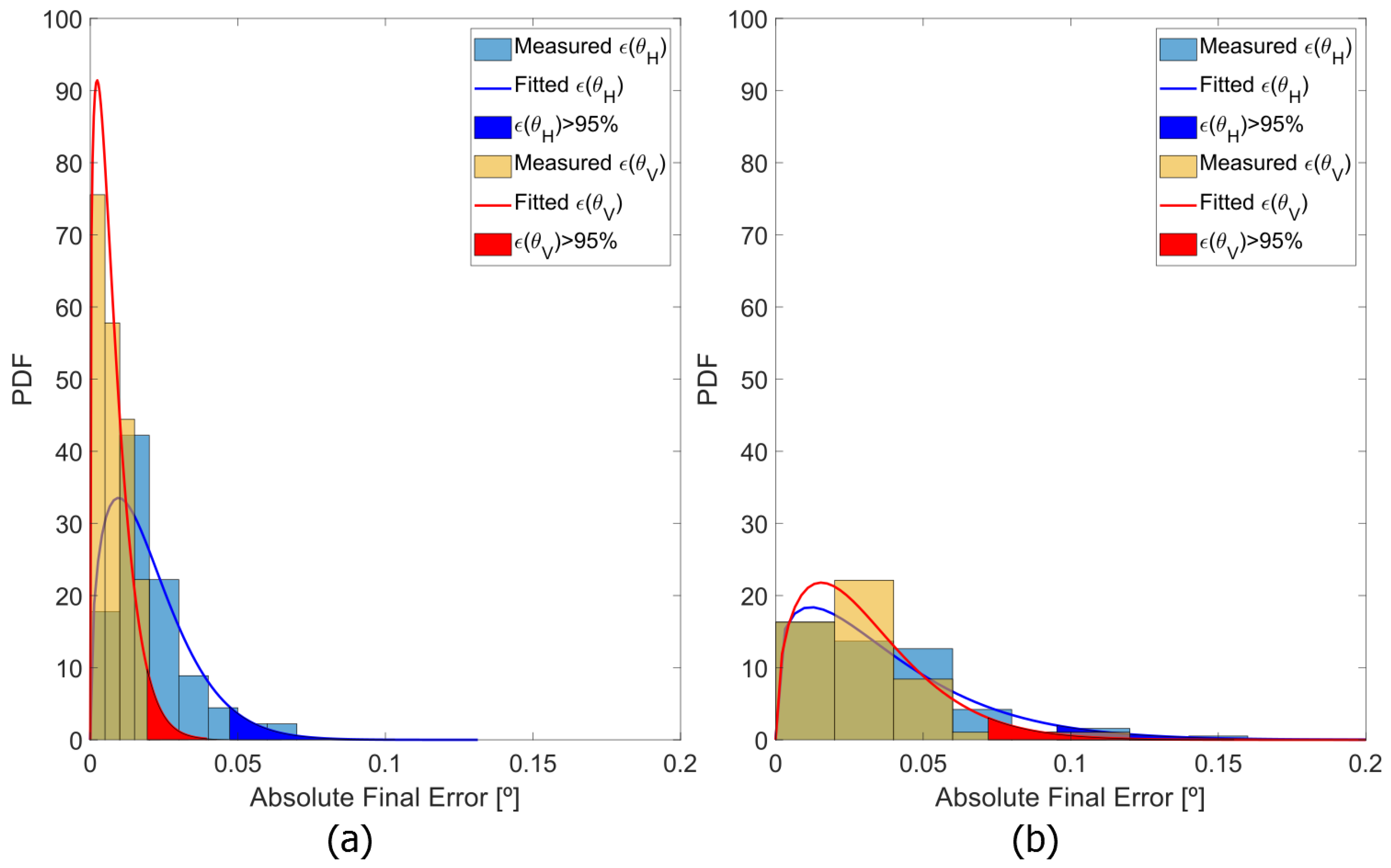
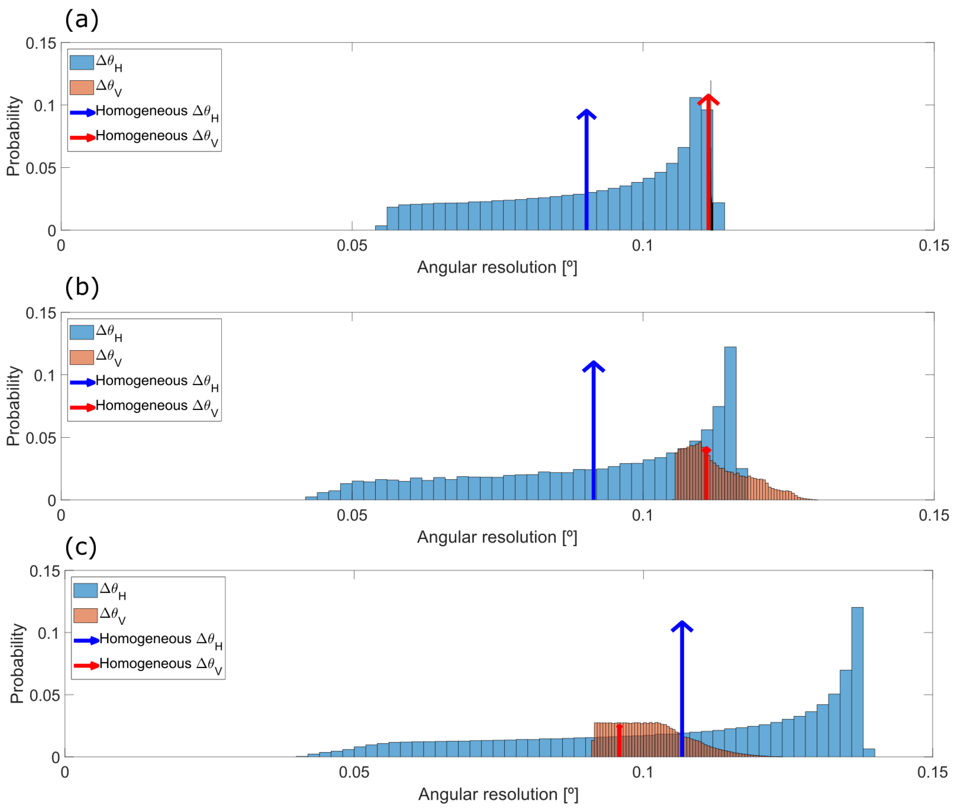
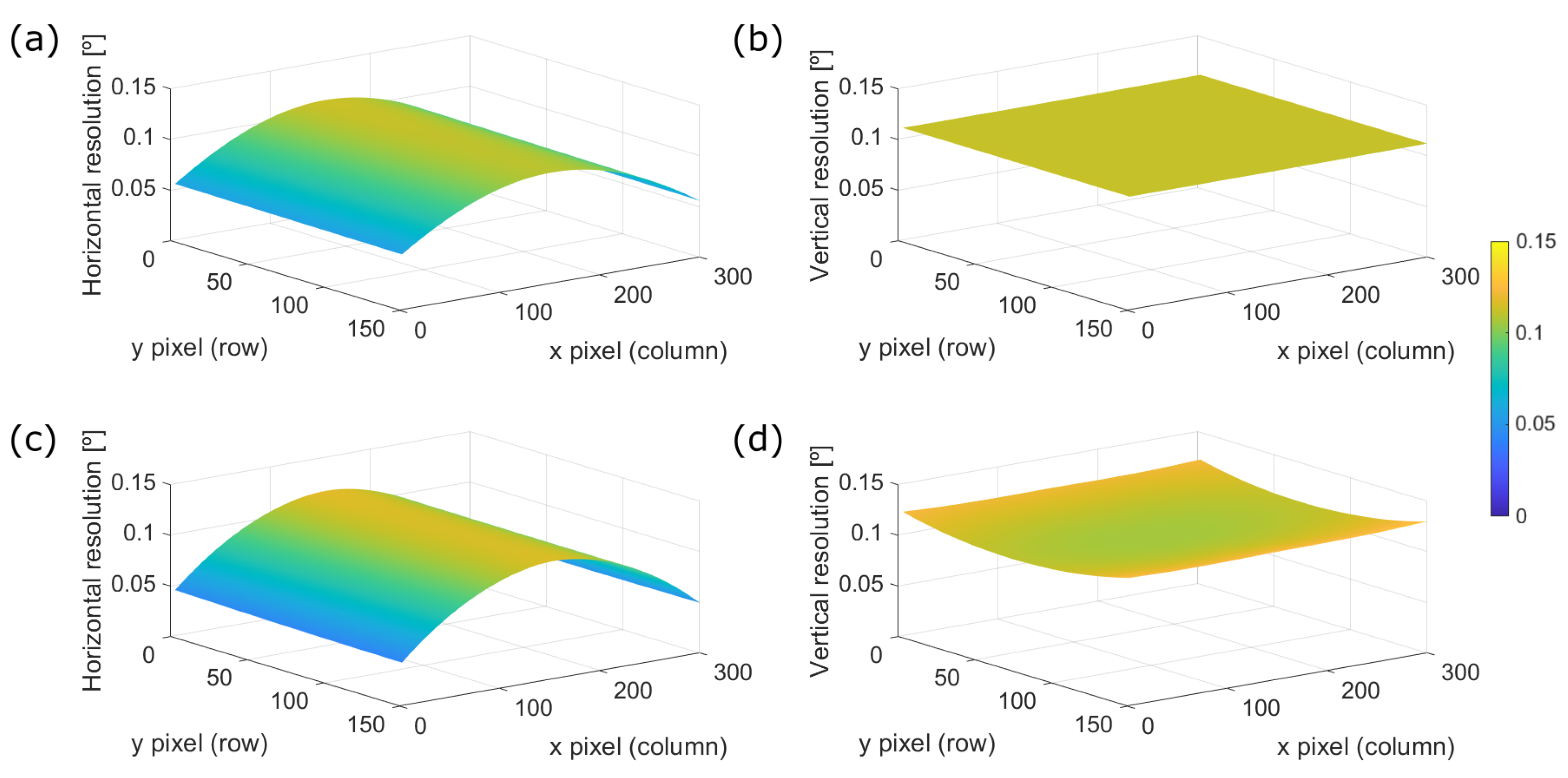
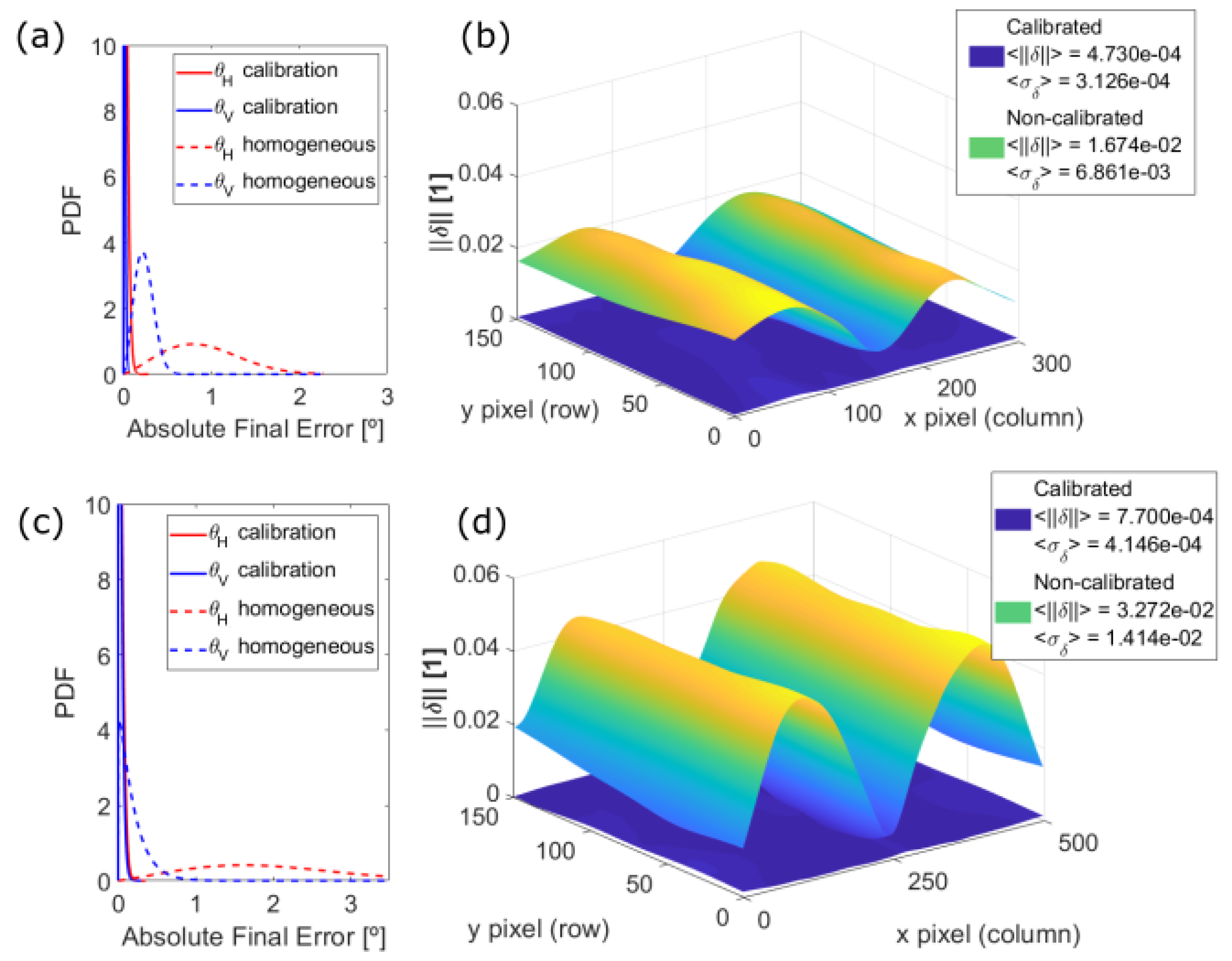
4.2. Calibration Results
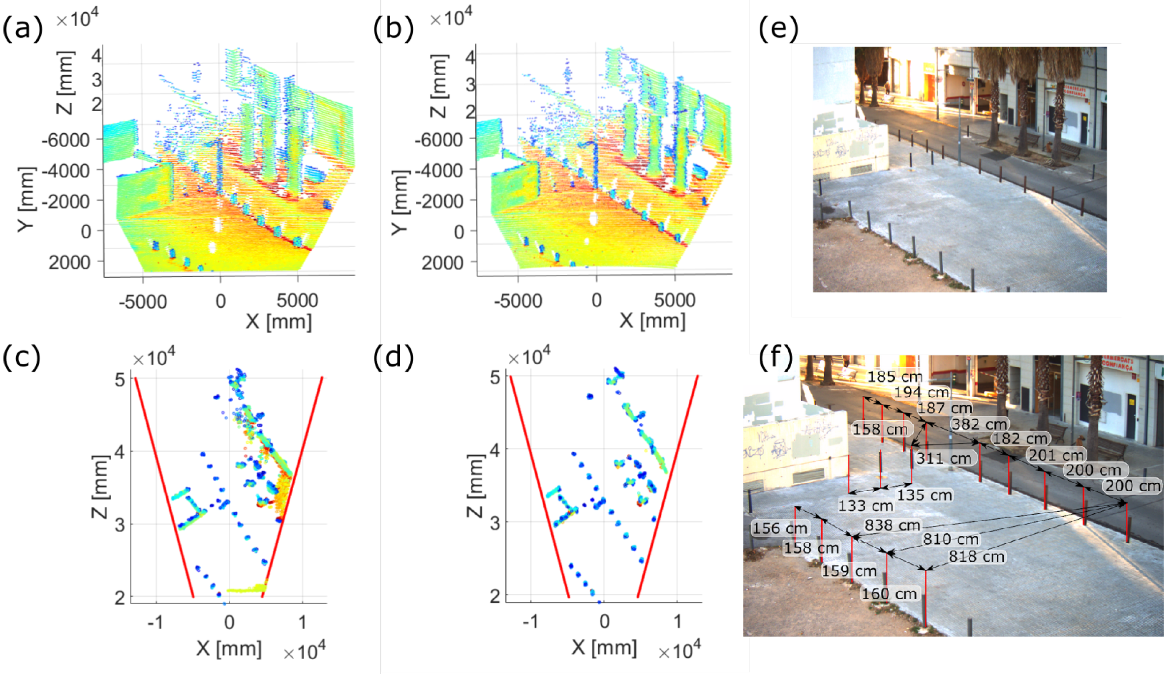
4.3. Impact on the Point Cloud
5. Conclusions
Author Contributions
Funding
Acknowledgments
Conflicts of Interest
Appendix A
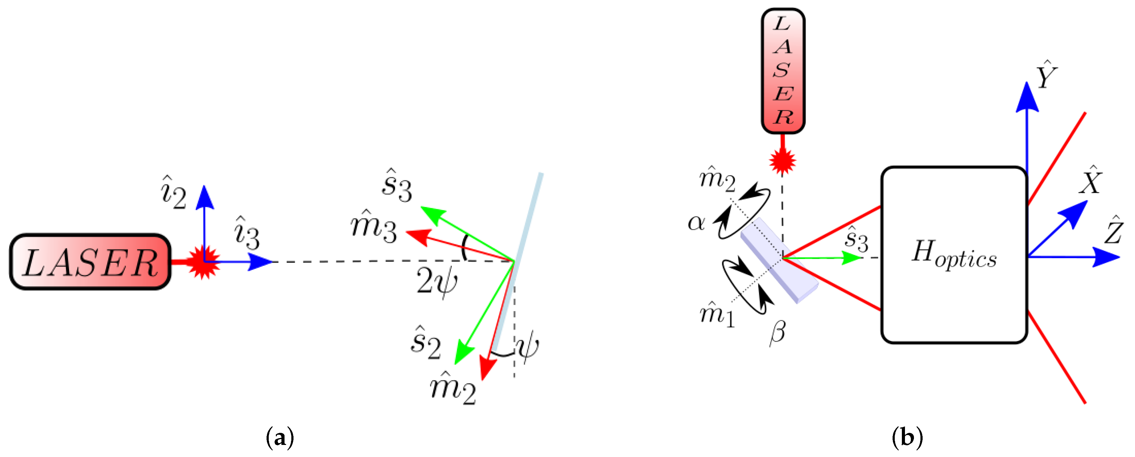
Appendix A.1. Vectorial Snell’s Law
Appendix A.2. Geometrical Model of MEMS Scanning
References
- Fernald, F.G. Analysis of atmospheric lidar observations: Some comments. Appl. Opt. AO 1984, 23, 652. [Google Scholar] [CrossRef] [PubMed]
- Korb, C.L.; Gentry, B.M.; Weng, C.Y. Edge technique: Theory and application to the lidar measurement of atmospheric wind. Appl. Opt. 1992, 31, 4202–4213. [Google Scholar] [CrossRef] [PubMed]
- McGill, M.J. Lidar Remote Sensing. In Encyclopedia of Optical Engineering; Marcel Dekker: New York, NY, USA, 2003; pp. 1103–1113. [Google Scholar]
- Liu, X. Airborne LiDAR for DEM generation: Some critical issues. Prog. Phys. Geogr. Earth Environ. 2008, 32, 31–49. [Google Scholar] [CrossRef]
- Mallet, C.; Bretar, F. Full-waveform topographic lidar: State-of-the-art. ISPRS J. Photogramm. Remote Sens. 2009, 64, 1–16. [Google Scholar] [CrossRef]
- Azuma, R.T.; Malibu, I. A Survey of Augmented Reality. Presence Teleoperators Virtual Environ. 1997, 6, 355–385. [Google Scholar] [CrossRef]
- Azuma, R.; Baillot, Y.; Behringer, R.; Feiner, S.; Julier, S.; MacIntyre, B. Recent advances in augmented reality. IEEE Comput. Graph. Appl. 2001, 21, 34–47. [Google Scholar] [CrossRef]
- Schwarz, B. LIDAR: Mapping the world in 3D. Nat. Photonics 2010, 4, 429–430. [Google Scholar] [CrossRef]
- Royo, S.; Ballesta-Garcia, M. An Overview of Lidar Imaging Systems for Autonomous Vehicles. Appl. Sci. 2019, 9, 4093. [Google Scholar] [CrossRef]
- Takagi, K.; Morikawa, K.; Ogawa, T.; Saburi, M. Road Environment Recognition Using On-vehicle LIDAR. In Proceedings of the 2006 IEEE Intelligent Vehicles Symposium, Tokyo, Japan, 13–15 June 2006; pp. 120–125. [Google Scholar] [CrossRef]
- Premebida, C.; Monteiro, G.; Nunes, U.; Peixoto, P. A Lidar and Vision-based Approach for Pedestrian and Vehicle Detection and Tracking. In Proceedings of the 2007 IEEE Intelligent Transportation Systems Conference, Seattle, WA, USA, 30 September–3 October 2007; pp. 1044–1049. [Google Scholar] [CrossRef]
- Gallant, M.J.; Marshall, J.A. The LiDAR compass: Extremely lightweight heading estimation with axis maps. Robot. Auton. Syst. 2016, 82, 35–45. [Google Scholar] [CrossRef]
- Huynh, D.Q.; Owens, R.A.; Hartmann, P.E. Calibrating a Structured Light Stripe System: A Novel Approach. Int. J. Comput. Vis. 1999, 33, 73–86. [Google Scholar] [CrossRef]
- Glennie, C.; Lichti, D.D. Static Calibration and Analysis of the Velodyne HDL-64E S2 for High Accuracy Mobile Scanning. Remote Sens. 2010, 2, 1610–1624. [Google Scholar] [CrossRef]
- Muhammad, N.; Lacroix, S. Calibration of a rotating multi-beam lidar. In Proceedings of the 2010 IEEE/RSJ International Conference on Intelligent Robots and Systems, Taipei, Taiwan, 18–22 October 2010; pp. 5648–5653. [Google Scholar] [CrossRef]
- Atanacio-Jiménez, G.; González-Barbosa, J.J.; Hurtado-Ramos, J.B.; Ornelas-Rodríguez, F.J.; Jiménez-Hernández, H.; García-Ramirez, T.; González-Barbosa, R. LIDAR Velodyne HDL-64E Calibration Using Pattern Planes. Int. J. Adv. Robot. Syst. 2011, 8, 59. [Google Scholar] [CrossRef]
- Mirzaei, F.M.; Kottas, D.G.; Roumeliotis, S.I. 3D LIDAR–camera intrinsic and extrinsic calibration: Identifiability and analytical least-squares-based initialization. Int. J. Robot. Res. 2012, 31, 452–467. [Google Scholar] [CrossRef]
- Yu, C.; Chen, X.; Xi, J. Modeling and Calibration of a Novel One-Mirror Galvanometric Laser Scanner. Sensors 2017, 17, 164. [Google Scholar] [CrossRef] [PubMed]
- Cui, S.; Zhu, X.; Wang, W.; Xie, Y. Calibration of a laser galvanometric scanning system by adapting a camera model. Appl. Opt. AO 2009, 48, 2632–2637. [Google Scholar] [CrossRef]
- Rodriguez, F.S.A.; Fremont, V.; Bonnifait, P. Extrinsic calibration between a multi-layer lidar and a camera. In Proceedings of the 2008 IEEE International Conference on Multisensor Fusion and Integration for Intelligent Systems, Seoul, Korea, 20–22 August 2008; pp. 214–219. [Google Scholar] [CrossRef]
- Kwak, K.; Huber, D.F.; Badino, H.; Kanade, T. Extrinsic calibration of a single line scanning lidar and a camera. In Proceedings of the 2011 IEEE/RSJ International Conference on Intelligent Robots and Systems, San Francisco, CA, USA, 25–30 September 2011; pp. 3283–3289. [Google Scholar]
- Zhou, L.; Deng, Z. Extrinsic calibration of a camera and a lidar based on decoupling the rotation from the translation. In Proceedings of the 2012 IEEE Intelligent Vehicles Symposium, Alcala de Henares, Spain, 3–7 June 2012; pp. 642–648. [Google Scholar] [CrossRef]
- García-Moreno, A.I.; Gonzalez-Barbosa, J.J.; Ornelas-Rodriguez, F.J.; Hurtado-Ramos, J.B.; Primo-Fuentes, M.N. LIDAR and Panoramic Camera Extrinsic Calibration Approach Using a Pattern Plane. In Pattern Recognition; Hutchison, D., Kanade, T., Kittler, J., Kleinberg, J.M., Mattern, F., Mitchell, J.C., Naor, M., Nierstrasz, O., Pandu Rangan, C., Steffen, B., et al., Eds.; Springer: Berlin/Heidelberg, Germany, 2013; Volume 7914, pp. 104–113. [Google Scholar] [CrossRef]
- Park, Y.; Yun, S.; Won, C.S.; Cho, K.; Um, K.; Sim, S. Calibration between Color Camera and 3D LIDAR Instruments with a Polygonal Planar Board. Sensors 2014, 14, 5333–5353. [Google Scholar] [CrossRef]
- Dhall, A.; Chelani, K.; Radhakrishnan, V.; Krishna, K.M. LiDAR-Camera Calibration using 3D-3D Point correspondences. arXiv 2017, arXiv:1705.09785. [Google Scholar]
- Guindel, C.; Beltrán, J.; Martín, D.; García, F. Automatic extrinsic calibration for lidar-stereo vehicle sensor setups. In Proceedings of the 2017 IEEE 20th International Conference on Intelligent Transportation Systems (ITSC), Yokohama, Japan, 16–19 October 2017; pp. 1–6. [Google Scholar] [CrossRef]
- Urey, H.; Holmstrom, S.; Baran, U. MEMS laser scanners: A review. J. Microelectromech. Syst. 2014, 23, 259. [Google Scholar] [CrossRef]
- Ortiz, S.; Siedlecki, D.; Grulkowski, I.; Remon, L.; Pascual, D.; Wojtkowski, M.; Marcos, S. Optical distortion correction in Optical Coherence Tomography for quantitative ocular anterior segment by three-dimensional imaging. Opt. Express OE 2010, 18, 2782–2796. [Google Scholar] [CrossRef]
- Brown, D.C. Decentering Distortion of Lenses. Photogramm. Eng. 1966, 32, 444–462. [Google Scholar]
- Swaninathan, R.; Grossberg, M.D.; Nayar, S.K. A perspective on distortions. In Proceedings of the 2003 IEEE Computer Society Conference on Computer Vision and Pattern Recognition, Madison, WI, USA, 18–20 June 2003; Volume 2. [Google Scholar] [CrossRef]
- Pan, B.; Yu, L.; Wu, D.; Tang, L. Systematic errors in two-dimensional digital image correlation due to lens distortion. Opt. Lasers Eng. 2013, 51, 140–147. [Google Scholar] [CrossRef]
- Bauer, A.; Vo, S.; Parkins, K.; Rodriguez, F.; Cakmakci, O.; Rolland, J.P. Computational optical distortion correction using a radial basis function-based mapping method. Opt. Express OE 2012, 20, 14906–14920. [Google Scholar] [CrossRef] [PubMed]
- Li, A.; Wu, Y.; Xia, X.; Huang, Y.; Feng, C.; Zheng, Z. Computational method for correcting complex optical distortion based on FOV division. Appl. Opt. AO 2015, 54, 2441–2449. [Google Scholar] [CrossRef] [PubMed]
- Sun, C.; Guo, X.; Wang, P.; Zhang, B. Computational optical distortion correction based on local polynomial by inverse model. Optik 2017, 132, 388–400. [Google Scholar] [CrossRef]
- Heikkila, J.; Silven, O. A four-step camera calibration procedure with implicit image correction. In Proceedings of the IEEE Computer Society Conference on Computer Vision and Pattern Recognition, San Juan, Puerto Rico, 17–19 June 1997; pp. 1106–1112. [Google Scholar] [CrossRef]


| Figure of Merit [Mdeg] | Dir. | 30 × 20 | 50 × 20 | ||||
|---|---|---|---|---|---|---|---|
| Map 1 | Map 2 | Map 3 | Map 1 | Map 2 | Map 3 | ||
| Homogeneous FOV [] | Odd | 27.55 × 16.32 | 27.47 × 16.54 | 27.47 × 16.52 | 52.89 × 13.96 | 53.19 × 14.44 | 53.34 × 14.38 |
| Even | 27.25 × 16.44 | 27.46 × 16.64 | 27.45 × 16.63 | 53.08 × 13.33 | 53.07 × 14.27 | 53.07 × 14.21 | |
| Mean error | Odd | 25 × 28 | 21 × 9 | 20 × 8 | 101 × 89 | 45 × 40 | 37 × 31 |
| Even | 23 × 24 | 22 × 9 | 22 × 9 | 108 × 118 | 47 × 64 | 46 × 37 | |
| Standard deviation | Odd | 24 × 23 | 14 × 5 | 14 × 5 | 66 × 97 | 34 × 32 | 29 × 22 |
| Even | 24 × 18 | 14 × 7 | 14 × 7 | 73 × 110 | 37 × 48 | 35 × 31 | |
| Max. angular error (<95%) | Odd | 79 × 70 | 48 × 17 | 47 × 19 | 239 × 274 | 117 × 103 | 95 × 72 |
| Even | 77 × 60 | 48 × 25 | 47 × 26 | 265 × 324 | 117 × 165 | 113 × 98 | |
© 2020 by the authors. Licensee MDPI, Basel, Switzerland. This article is an open access article distributed under the terms and conditions of the Creative Commons Attribution (CC BY) license (http://creativecommons.org/licenses/by/4.0/).
Share and Cite
García-Gómez, P.; Royo, S.; Rodrigo, N.; Casas, J.R. Geometric Model and Calibration Method for a Solid-State LiDAR. Sensors 2020, 20, 2898. https://doi.org/10.3390/s20102898
García-Gómez P, Royo S, Rodrigo N, Casas JR. Geometric Model and Calibration Method for a Solid-State LiDAR. Sensors. 2020; 20(10):2898. https://doi.org/10.3390/s20102898
Chicago/Turabian StyleGarcía-Gómez, Pablo, Santiago Royo, Noel Rodrigo, and Josep R. Casas. 2020. "Geometric Model and Calibration Method for a Solid-State LiDAR" Sensors 20, no. 10: 2898. https://doi.org/10.3390/s20102898
APA StyleGarcía-Gómez, P., Royo, S., Rodrigo, N., & Casas, J. R. (2020). Geometric Model and Calibration Method for a Solid-State LiDAR. Sensors, 20(10), 2898. https://doi.org/10.3390/s20102898