Regiomontan: A Regional High Precision Ionosphere Delay Model and Its Application in Precise Point Positioning


Abstract
1. Introduction
2. Estimating the Ionospheric Delay from GNSS Observations
3. Development of a Regional High Precision Ionosphere Delay Model
3.1. Taylor Approximation of the Single-Layer Model
3.2. Parameter Estimation Using Code-Leveled Carrier-Phase Observations
3.3. Specifications of the Output Files in IONEX Format
4. Applying the Regiomontan Model to Precise Point Positioning
4.1. Classical PPP Model
4.2. Uncombined PPP Model with Ionospheric Constraint
5. Results
5.1. Validating Regiomontan via Ionosphere-Free Linear Combination
5.2. PPP Results with Regiomontan
6. Conclusions
Author Contributions
Funding
Acknowledgments
Conflicts of Interest
References
- Rishbeth, H.; Garriott, O. Introduction to Ionospheric Physics; Academic Press: New York, NY, USA, 1969. [Google Scholar]
- Böhm, J.; Salstein, D.; Alizadeh, M.M.; Wijaya, D.D. Geodetic and Atmospheric Background. In Atmopheric Effects in Space Geodesy; Böhm, J., Schuh, H., Eds.; Springer: Vienna, Austria, 2013; pp. 1–33. [Google Scholar]
- Klobuchar, J.A. Ionospheric Time-Delay algorithm for Single-Frequency GPS Users. IEEE Trans. Aerosp. Electron. Syst. 1987, 3, 325–331. [Google Scholar] [CrossRef]
- Van Dierendonck, A.J.; Russell, S.S.; Kopitzke, E.R.; Birnbaum, M. The GPS Navigation Message. Navigation 1978, 25, 147–165. [Google Scholar] [CrossRef]
- Hochegger, G.; Nava, B.; Radicella, S.M.; Leitinger, R. A family of ionospheric models for different uses. Phys. Chem. Earth Part C Sol. Terr. Planet. Sci. 2000, 25, 307–310. [Google Scholar] [CrossRef]
- Radicella, S.M.; Leitinger, R. The evolution of the DGR approach to model electron density profiles. Adv. Space Res. 2001, 27, 35–40. [Google Scholar] [CrossRef]
- Di Giovanni, G.; Radicella, S.M. An analytical model of the electron density profile in the ionosphere. Adv. Space Res. 1990, 10, 27–30. [Google Scholar] [CrossRef]
- Nava, B.; Coïsson, P.; Radicella, S.M. A new version of the NeQuick ionosphere electron density model. J. Atmos. Sol. Terr. Phys. 2008, 70, 1856–1862. [Google Scholar] [CrossRef]
- Hoque, M.M.; Jakowski, N.; Osechas, O.; Berdermann, J. Fast and improved ionospheric correction for Galileo mass market receivers. In Proceedings of the 32nd International Technical Meeting of the Satellite Division of The Institute of Navigation (ION GNSS+ 2019), Miami, FL, USA, 16–20 September 2019; pp. 3377–3389. [Google Scholar] [CrossRef]
- Johnston, G.; Riddell, A.; Hausler, G. The International GNSS Service. In Springer Handbook of Global Navigation Satellite Systems; Teunissen, P.J.G., Montenbruck, O., Eds.; Springer International Publishing: Cham, Switzerland, 2017; pp. 967–982. [Google Scholar]
- Jakowski, N.; Porsch, F.; Mayer, G. Ionosphere-induced-ray-path bending effects in precise satellite positioning systems. Zeitschrift für Satellitengestützte Positionierung, Navigation und Kommunikation 1994, 94, 6–13. [Google Scholar]
- Hoque, M.M.; Jakowski, N. Higher order ionospheric effects in precise GNSS positioning. J. Geod. 2007, 81, 259–268. [Google Scholar] [CrossRef]
- Aragon-Angel, A.; Hernandes-Pajares, M.; Defraigne, P.; Bergeot, N.; Prieto-Cerdeira, R. Modelling and assessing ionospheric higher order terms for GNSS signals. In Proceedings of the 28th International Technical Meeting of the ION Satellite Division, ION GNSS+ 2015, Tampa, FL, USA, 14–18 September 2015; pp. 3511–3524. [Google Scholar]
- Rovira-Garcia, A.; Juan, J.M.; Sanz, J. A Real-time World-wide Ionospheric Model for Single and Multi-frequency Precise Navigation. In Proceedings of the 27th International Technical Meeting of the ION Satellite Division, ION GNSS+ 2014, Tampa, FL, USA, 8–12 September 2014; pp. 2533–2543. [Google Scholar]
- Hernández-Pajares, M.; Roma-Dollase, D.; Garcia-Fernàndez, M.; Orus-Perez, R.; García-Rigo, A. Precise ionospheric electron content monitoring from single-frequency GPS receivers. GPS Solut. 2018, 22, 102. [Google Scholar] [CrossRef]
- Li, Z.; Wang, N.; Hernández-Pajares, M.; Yuan, Y.; Krankowski, A.; Liu, A.; Zha, J.; García-Rigo, A.; Roma-Dollase, D.; Yang, H.; et al. IGS real-time service for global ionospheric total electron content modeling. J. Geod. 2020, 94, 32. [Google Scholar] [CrossRef]
- Weber, R.; Boisits, J.; Joldzic, N.; Umnig, E.; Klug, C.; Thaler, G.; Karas, R. Regiomontan-Regionale Ionosphärenmodellierung für Einfrequenz-Nutzer Anwendungen; Technical Report; E120-Department of Geodesy and Geoinformation: TU Wien, Austria, 2016. [Google Scholar]
- Boisits, J.; Joldzic, N.; Weber, R. Regional Ionospheric Modelling for Single-Frequency Users. Geophys. Res. Abstr. 2016, 18, 2016–6322. [Google Scholar]
- Böhm, J.; Böhm, S.; Boisits, J.; Girdiuk, A.; Gruber, J.; Hellerschied, A.; Krásná, H.; Landskron, D.; Madzak, M.; Mayer, D.; et al. Vienna VLBI and Satellite Software (VieVS) for Geodesy and Astrometry. Publ. Astron. Soc. Pac. 2018, 130, 044503. [Google Scholar] [CrossRef]
- Zumberge, J.F.; Heflin, M.B.; Jefferson, D.C.; Watkins, M.M.; Webb, F.H. Precise point positioning for the efficient and robust analysis of GPS data from large networks. J. Geophys. Res. Solid Earth 1997, 102, 5005–5017. [Google Scholar] [CrossRef]
- Lou, Y.; Zheng, F.; Gu, S.; Wang, C.; Guo, H.; Feng, Y. Multi-GNSS precise point positioning with raw single-frequency and dual-frequency measurement models. GPS Solut. 2016, 20, 849–862. [Google Scholar] [CrossRef]
- De Bakker, P.F. On User Algorithms for GNSS Precise Point Positioning. Ph.D. Thesis, Delft University of Technology, Delft, The Netherlands, 2016. [Google Scholar]
- Shi, C.; Gu, S.; Lou, Y.; Ge, M. An improved approach to model ionospheric delays for single-frequency Precise Point Positioning. Adv. Space Res. 2012, 49, 1698–1708. [Google Scholar] [CrossRef]
- Ning, Y.; Han, H.; Zhang, L. Single-frequency precise point positioning enhanced with multi-GNSS observations and global ionosphere maps. Meas. Sci. Technol. 2019, 30, 015013. [Google Scholar] [CrossRef]
- Aggrey, J.; Bisnath, S. Improving GNSS PPP Convergence: The Case of Atmospheric-Constrained, Multi-GNSS PPP-AR. Sensors 2019, 19, 587. [Google Scholar] [CrossRef]
- Wang, R.; Gao, J.; Zheng, N.; Li, Z.; Yao, Y.; Zhao, L.; Wang, Y. Research on Accelerating Single-Frequency Precise Point Positioning Convergence with Atmospheric Constraint. Appl. Sci. 2019, 9, 5407. [Google Scholar] [CrossRef]
- Zhou, F.; Dong, D.; Li, W.; Jiang, X.; Wickert, J.; Schuh, H. GAMP: An open-source software of multi-GNSS precise point positioning using undifferenced and uncombined observations. GPS Solut. 2018, 22, 33. [Google Scholar] [CrossRef]
- Cai, C.; Gong, Y.; Gao, Y.; Kuang, C. An Approach to Speed up Single-Frequency PPP Convergence with Quad-Constellation GNSS and GIM. Sensors 2017, 17, 1302. [Google Scholar] [CrossRef]
- Bassiri, S.; Hajj, G. Higher-order ionospheric effects on the global positioning system observables and means of modeling them. Manuscripta Geod. 1993, 18, 280–289. [Google Scholar]
- Fritsche, M.; Dietrich, R.; Knöfel, C.; Rülke, A.; Vey, S.; Rothacher, M.; Steigenberger, P. Impact of higher-order ionospheric terms on GPS estimates. Geophys. Res. Lett. 2005, 32, L23311. [Google Scholar] [CrossRef]
- Alizadeh, M.M.; Wijaya, D.D.; Hobiger, T.; Weber, R.; Schuh, H. Ionospheric Effects on Microwave Signals. In Atmopheric Effects in Space Geodesy; Böhm, J., Schuh, H., Eds.; Springer: Vienna, Austria, 2013; pp. 35–71. [Google Scholar]
- Hoque, M.M.; Jakowski, N. A new global model for the ionospheric F2 peak height for radio wave propagation. Ann. Geophys. 2012, 30, 797–809. [Google Scholar] [CrossRef]
- Schaer, S. Mapping and predicting the Earth’s ionosphere using the Global Positioning System. Ph.D. Thesis, Bern University, Bern, Switzerland, 1999. [Google Scholar]
- Schaer, S.; Gurtner, W.; Feltens, J. IONEX: The IONosphere Map EXchange Format Version 1. In Proceedings of the IGS AC Workshop, Darmstadt, Germany, 9–11 February 1998. [Google Scholar]
- EPOSA—Echtzeit Positionierung Austria. Available online: http://www.eposa.at/ (accessed on 15 May 2020).
- Banville, S.; Zhang, W.; Langley, R.B. Monitoring the Ionosphere with Integer-Leveled GPS Measurements. GPS World 2013, 24, 43–49. [Google Scholar]
- De Jonge, P.J. A Processing Strategy for the Application of the GPS in Networks. Ph.D. Thesis, Delft University of Technology, Delft, The Netherlands, 1998. [Google Scholar]
- Teunissen, P.J.G.; Khodabandeh, A. Review and principles of PPP-RTK methods. J. Geod. 2015, 89, 217–240. [Google Scholar] [CrossRef]
- Kouba, J. A Guide to Using INTERNATIONAL GNSS Service (IGS) Products. Available online: http://acc.igs.org/UsingIGSProductsVer21.pdf (accessed on 30 March 2020).
- Zhang, H.; Gao, Z.; Ge, M.; Niu, X.; Huang, L.; Tu, R.; Li, X. On the Convergence of Ionospheric Constrained Precise Point Positioning (IC-PPP) Based on Undifferential Uncombined Raw GNSS Observations. Sensors 2013, 13, 15708–15725. [Google Scholar] [CrossRef]
- Odijk, D.; Zhang, B.; Khodabandeh, A.; Odolinski, R.; Teunissen, P.J.G. On the estimability of parameters in undifferenced, uncombined GNSS network and PPP-RTK user models by means of S-system theory. J. Geod. 2016, 90, 15–44. [Google Scholar] [CrossRef]
- Liu, T.; Wang, J.; Yu, H.; Cao, X.; Ge, Y. A New Weighting Approach with Application to Ionospheric Delay Constraint for GPS/GALILEO Real-Time Precise Point Positioning. Appl. Sci. 2018, 8, 2537. [Google Scholar] [CrossRef]
- Dach, R.; Schaer, S.; Arnold, D.; Prange, L.; Sidorov, D.; Stebler, P.; Villiger, A.; Jäggi, A. CODE Final Product Series for the IGS; Astronomical Institute: Miyagi, Japan, 2018. [Google Scholar]
- Rebischung, O.; Schmid, R. IGS14/igs14.atx: A new framework for the IGS products [poster]. In Proceedings of the AGU Fall Meeting 2016, San Francisco, CA, USA, 12–16 December 2016. [Google Scholar]
- Landskron, D.; Böhm, J. VMF3/GPT3: Refined Discrete and Empirical Troposphere Mapping Functions. J. Geod. 2018, 92, 349–360. [Google Scholar] [CrossRef]
- Ihde, J.; Habrich, H.; Sacher, M.; Söhne, W.; Altamimi, Z.; Brockmann, E.; Bruyninx, C.; Caporali, A.; Dousa, J.; Fernandes, R.; et al. EUREF’s Contribution to National, European and Global Geodetic Infrastructures. In Earth on the Edge: Science for a Sustainable Planet; Rizos, C., Willis, P., Eds.; Springer: Berlin/Heidelberg, Germany, 2014; pp. 189–196. [Google Scholar]
- Wu, J.T.; Wu, S.C.; Hajj, G.A.; Bertiger, W.; Lichten, S. Effects of antenna orientation on GPS carrier phase. Manuscripta Geod. 1993, 18, 91–98. [Google Scholar]
- Petit, G.; Luzum, B. (Eds.) IERS Conventions (2010). In IERS Technical Note; Number 36; Verlag des Bundesamts für Kartographie und Geodäsie: Frankfurt am Main, Germany, 2010; pp. 99–119. [Google Scholar]
- Springer, T.; Hugentobler, U. IGS ultra rapid products for (near-) real-time applications. Phys. Chem. Earth Part A Solid Earth Geod. 2001, 26, 623–628. [Google Scholar] [CrossRef]


| Specification | Value |
|---|---|
| # of maps | 25 (00:00 UTC–00:00 UTC) |
| Interval | 3600 s |
| Latitude: min, max | 30°, 70° |
| Longitude: min, max | −20°, 45° |
| Spatial resolution | 1° × 1° |
| GPS Week 2056 | GPS Week 2082 | |||||||
|---|---|---|---|---|---|---|---|---|
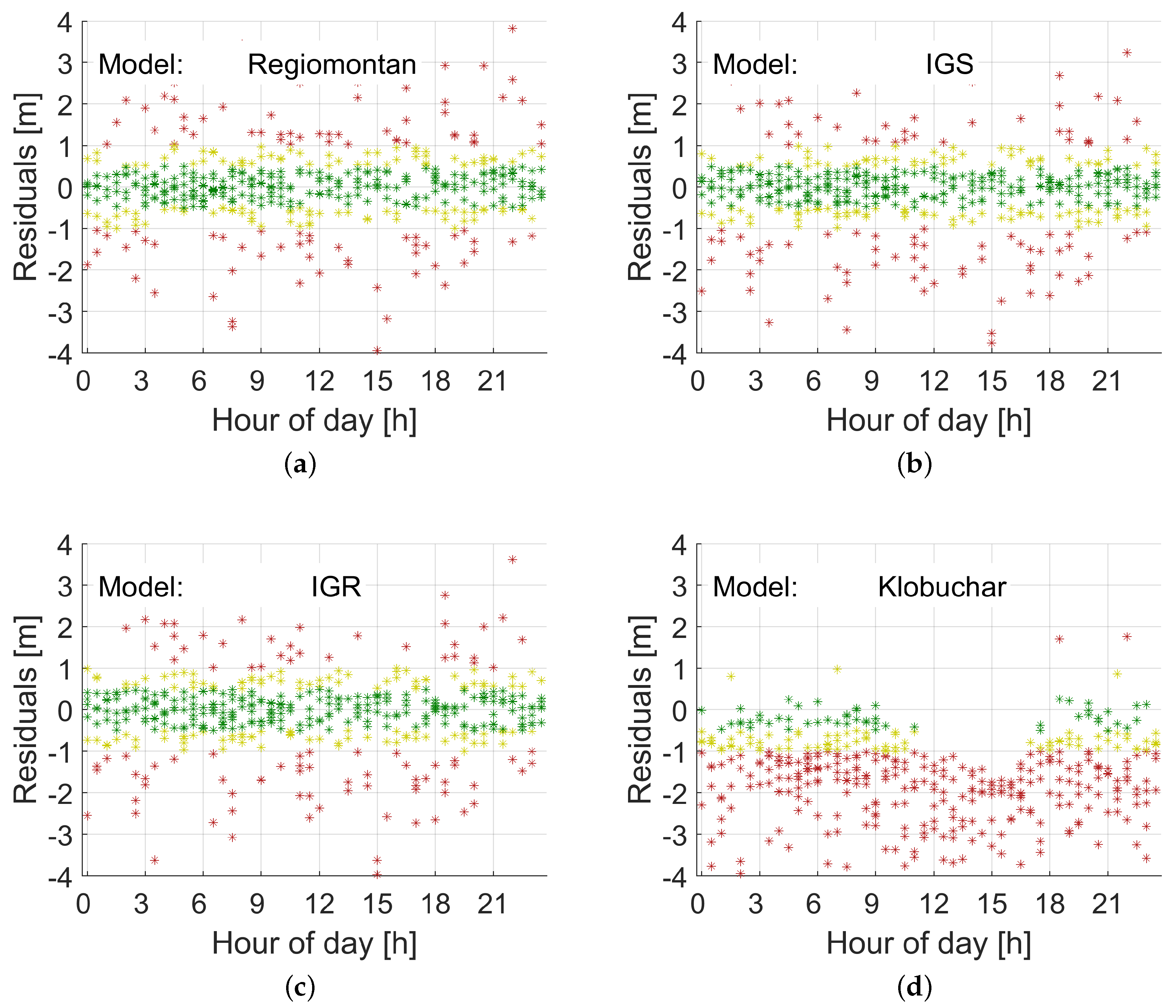
| Residuals | Regiomontan | IGS | IGR | Klobuchar | Regiomontan | IGS | IGR | Klobuchar |
| <0.5 m | 52.0% | 49.3% | 49.2% | 24.7% | 53.9% | 52.5% | 51.0% | 13.0% |
| <1.0 m | 76.4% | 74.0% | 73.9% | 45.3% | 79.7% | 78.7% | 77.6% | 30.1% |
| <1.5 m | 87.3% | 85.1% | 85.1% | 61.0% | 90.0% | 89.4% | 88.6% | 49.0% |
| Setting | Value |
|---|---|
| Stations | GRAZ, PFA3, LINZ, SBG2, TRF2 |
| Period | June 2019, December 2019 |
| GNSS | GPS, Glonass (weighted 1:1) |
| GPS Observations | L1, L2 |
| Glonass Observations | G1, G2 |
| Processing mode | undifferenced observations, static receiver |
| Observation interval | 30 s, reset solution: every full hour |
| Raw observation noise | code = 30 cm, phase = 2 mm |
| Observation weighting | Elevation weighted () |
| Cutoff angle | elevation: 5° |
| Satellite Orbits, Clocks and DCBs | CODE final products [43] |
| Satellite and receiver antenna | IGS Antex igs14.atx [44] |
| Troposphere model | VMF3 [45], residual ZWD is estimated |
| Reference coordinates | EUREF [46] |
| Adjustment | Kalman-Filter |
| Receiver clock, time offset | white noise |
| Phase Ambiguities | float, constant |
| Cycle-Slip Detection | dL1-dL2 |
| Correction models | Phase wind-up [47], solid earth tides [48], relativistic effects |
| 5 min | 10 min | 15 min | 30 min | 45 min | |
|---|---|---|---|---|---|
| IF LC | 45.2 | 18.1 | 8.7 | 4.9 | 3.8 |
| REGIO | 39.6 | 16.6 | 8.0 | 4.8 | 3.8 |
| IGS | 39.1 | 16.5 | 8.0 | 4.7 | 3.8 |
| CODE | 39.0 | 16.4 | 7.9 | 4.8 | 3.8 |
| GNSS | GPS | Glonass | ||||
|---|---|---|---|---|---|---|
| Model | REGIO | IGS | CODE | REGIO | IGS | CODE |
| Month | June | |||||
| <12.5 cm | 42.6% | 43.4% | 49.7% | 27.5% | 30.7% | 31.8% |
| <25 cm | 69.1% | 71.4% | 76.6% | 50.6% | 56.8% | 57.9% |
| <50 cm | 89.7% | 92.0% | 93.4% | 77.4% | 85.7% | 86.2% |
| Month | December | |||||
| <12.5 cm | 41.2% | 43.9% | 47.5% | 30.2% | 34.6% | 41.7% |
| <25 cm | 68.7% | 73.2% | 74.9% | 53.8% | 60.1% | 68.3% |
| <50 cm | 90.1% | 93.0% | 92.2% | 80.1% | 87.6% | 89.5% |
© 2020 by the authors. Licensee MDPI, Basel, Switzerland. This article is an open access article distributed under the terms and conditions of the Creative Commons Attribution (CC BY) license (http://creativecommons.org/licenses/by/4.0/).
Share and Cite
Boisits, J.; Glaner, M.; Weber, R. Regiomontan: A Regional High Precision Ionosphere Delay Model and Its Application in Precise Point Positioning. Sensors 2020, 20, 2845. https://doi.org/10.3390/s20102845
Boisits J, Glaner M, Weber R. Regiomontan: A Regional High Precision Ionosphere Delay Model and Its Application in Precise Point Positioning. Sensors. 2020; 20(10):2845. https://doi.org/10.3390/s20102845
Chicago/Turabian StyleBoisits, Janina, Marcus Glaner, and Robert Weber. 2020. "Regiomontan: A Regional High Precision Ionosphere Delay Model and Its Application in Precise Point Positioning" Sensors 20, no. 10: 2845. https://doi.org/10.3390/s20102845
APA StyleBoisits, J., Glaner, M., & Weber, R. (2020). Regiomontan: A Regional High Precision Ionosphere Delay Model and Its Application in Precise Point Positioning. Sensors, 20(10), 2845. https://doi.org/10.3390/s20102845