Deep Learning Based Switching Filter for Impulsive Noise Removal in Color Images

Abstract

Noise reduction is one of the most important and still active research topics in low-level image processing due to its high impact on object detection and scene understanding for computer vision systems. Recently, we observed a substantially increased interest in the application of deep learning algorithms. Many computer vision systems use them, due to their impressive capability of feature extraction and classification. While these methods have also been successfully applied in image denoising, significantly improving its performance, most of the proposed approaches were designed for Gaussian noise suppression. In this paper, we present a switching filtering technique intended for impulsive noise removal using deep learning. In the proposed method, the distorted pixels are detected using a deep neural network architecture and restored with the fast adaptive mean filter. The performed experiments show that the proposed approach is superior to the state-of-the-art filters designed for impulsive noise removal in color digital images.

1. Introduction

Image denoising is a long-standing research topic in low-level image processing that still receives much attention from the computer vision community [1,2]. Over the last three decades, a considerable increase in the effectiveness of algorithms took place, but despite these improvements, modern miniaturized high-resolution, low-cost image sensors still provide a limited quality, when operating in poor lighting conditions. Therefore, image enhancement and noise removal are very important operations of digital image processing [3,4].

In practice, we can observe various types of noise that significantly degrade the quality of captured images. One of them is the so-called impulsive noise, which may appear due to electric signal instabilities, corruptions in physical memory storage, random or systematic errors in data transmission, electromagnetic interferences, malfunctioning or aging of camera sensors and low lighting conditions [3,5,6,7]. This type of noise causes a total loss of information at certain image locations because the original color channels information is replaced by random values.

In the literature, impulse noise is typically classified into two main categories [8,9,10]. The first one is the Channel Together Random Impulse (CTRI), in which a pixel channel may be replaced with any value in the image intensity range. The second noise model is salt and pepper impulse noise, in which a corrupted pixel value is set to either the minimum or the maximum of a range of possible values (so it is set to either 0 or 255 for an 8-bit image). In both models, the main parameter is the noise density $\rho$, which is the fraction of corrupted pixels in the processed image. In this paper, we focus on the CTRI model, however the proposed filter can also be applied to the salt and pepper model.

The classical method for removal of impulsive noise is the median filter. Generally, the median concept for color images is based on vector ordering, in which image pixels are treated as three-dimensional vectors. Such an approach yields better results than processing image channels independently [11,12,13,14], as the strong correlation between color channels is considered. The most widely used denoising method based on the ordering concept is the Vector Median Filter (VMF) [15], whose drawback is that every pixel of the image is processed, regardless of whether it is contaminated or not. This may result in strong signal degradation and introduction of perceivable blurring effect, especially in highly textured regions. In many applications, it may become a major flaw, and therefore, a plethora of improvements have been proposed [6,16,17,18,19,20,21,22,23,24,25].

To preserve image details and still efficiently suppress impulsive noise, a family of filters based on fuzzy set theory was also introduced, in which a combination of noise detection and a replacement scheme based on weighted averaging is performed [26,27,28,29,30,31]. However, these methods still may alter clean pixels in the processed image. An effective approach to retain uncorrupted pixels is based on the switching concept [32]. A general scheme of switching filter is presented in Figure 1. In the majority of the switching techniques, it is necessary to determine the measure of the impulsiveness of the processed pixel, which allows classifying the pixels as pristine or distorted. One of the most popular measures of similarity used in switching filters is the ROAD (Rank-Ordered Absolute Differences) statistic introduced in [33], in which the trimmed cumulative distance of the pixels, in a given color space, to their neighbors is utilized as a degree of pixel corruption.

Among switching filters, an important group of methods is based on the concept of a peer group [34,35,36], in which the membership degree of a central pixel of the filtering window to its local neighborhood is determined in terms of the number of close pixels. Another efficient family utilizes the elements of quaternion theory [37,38]. In this concept, instead of the commonly used Euclidean distance in a chosen color space, the similarity between pixels is defined in the quaternion form. Some switching filters also use classical machine learning approaches for impulse detection such as Support Vector Machines [39] and fully connected neural networks [40,41,42,43]. The detected impulses are restored using a median of neighboring uncorrupted pixels [40,42], adaptive and iterative mean filters [41] or edge-preserving regularization methods [43].

Recently, thanks to easy access to large image datasets and advances in deep learning, the Convolutional Neural Networks (CNNs) have led to a series of breakthroughs in various computer vision problems such as image segmentation, object recognition and detection. Concurrently, CNNs have also been successfully applied for image denoising, focusing mainly on the problem of Gaussian noise suppression. The recently proposed filters significantly outperform classical, well established algorithms in terms of filtering efficiency and computational speed [44,45,46]. However, despite the fact that image denoising using deep learning for Gaussian noise removal has been well-studied, relatively little work has been done in the area of impulsive noise detection and removal [47,48,49,50,51]. In [47], the authors proposed a method, which replaces noisy image pixels by a weighted average of samples from the neighborhood to remove salt and pepper noise and then the filter output is further processed using CNN to boost the final filtering performance. An alternative technique [48] divides the input image into small patches, which are processed independently by a set of convolution and deconvolution layers. Yet another approach [50] is based on a CNN trained on noisy images and is using the ROAD statistic to estimate the contamination level and to select the network found to be optimal for the estimated image pollution. The authors of [51] proposed to use two CNNs: the first one detects noisy pixels and the second one performs the final image reconstruction.

In one of the most promising approaches, called Denoising Convolutional Neural Network (DnCNN) [52], the authors proved that residual learning and batch normalization are beneficial in the case of the Gaussian noise model. Unfortunately, the network based on residual learning formulation is not effective in the case of other types of operations like JPEG artifacts removal, deblurring or image resolution enhancement [53] and also in the case of impulsive noise suppression. Applying residual learning for images contaminated by impulsive noise causes all pixels in the image to be altered, even those that were impulse-free, introducing unpleasant visual artifacts. Moreover, impulsive noise is not additive, and therefore, a residual approach is not suitable. To alleviate the inability of DnCNN to cope with impulsive distortions, we propose a modified version, which will be denoted as Impulse Detection Convolutional Neural Network (IDCNN).

In the proposed approach, we added a sigmoid layer to distinguish noise-free pixels from impulses and we reformulated the residual learning to the classification problem. In this way, the deep neural network is used as the impulse detector, and afterward, the corrupted pixels are restored using an adaptive mean filter, due to its good balance between computational complexity and restoration efficacy. The main contributions of our paper are as follows:

• We introduce a CNN architecture for impulse detection in noisy images,
• We propose a switching filter that applies deep learning for the localization of corrupted pixels and adaptive mean technique for their replacement,
• We analyze the impact of some network’s parameters on impulse detection accuracy,
• We also investigate the influence of impulse detection errors on the final restoration efficiency,
• We show that the proposed method is superior to the state-of-the-art denoising algorithms,
• We share the source code of the proposed approach at http://github.com/k-radlak/IDCNN.

The paper is organized as follows. Section 2 describes the structure of the proposed switching filter, focusing on the architecture of the proposed IDCNN and also presents its ablation study and the applied noisy pixel replacement method. The next section presents a comparison of the proposed technique with state-of-the-art filters designed for impulsive noise removal. Finally, discussion and conclusions are given in Section 4.

2. Proposed Switching Filter Design

Recently, the application of deep learning for image denoising has received much attention from the computer vision community due to its significant performance improvement in comparison to the classical machine learning algorithms. One of the most interesting methods, intended for Gaussian noise suppression, is the Denoising Convolutional Neural Network (DnCNN), inspired by VGG network [54] and introduced by Zhang et al. [52].

The DnCNN contains a sequence of convolutional layers followed by Rectified Linear Unit (ReLU) [55] and Batch Normalization (BN) [56]. The first layer has a convolution filter and ReLU activation. The second and each consecutive layer consists of a convolution filter, BN and ReLU activation, with the exception of the last layer that only uses convolution. The training of the network is based on the concept of deep residual learning [57], in which the network does not estimate the original values of the undistorted image, but instead learns to estimate the difference between a noisy and clean image.

The DnCNN filter outperforms most of the state-of-the-art algorithms designed for Gaussian noise reduction, but due to the fact that it uses residual learning, the original DnCNN trained on impulsive noise model also alters non-corrupted pixels as was shown in [49]. Therefore, in the proposed IDCNN, we modified the original DnCNN architecture to ensure that noise-free pixels will not be affected.

2.1. Impulsive Noise Detection Using CNN

In our approach, instead of the usage of residual learning, we employed all layers proposed in DnCNN for feature extraction and we added a sigmoid layer, which estimates for each pixel its impulsivity measure $\pi \in [0,1]$, the values of which are close to 0 when a pixel is likely to be undistorted and close to 1 if it seems to be corrupted. In this way, the network divides the image pixels into clean and distorted, depending on the appropriate value of the $\pi$ measure. The pixels with $\pi =0$ or $\pi =1$, are treated by the network as clean or corrupted respectively, with highest confidence. The architecture of the proposed network is depicted in Figure 2.

The introduced architecture also requires a change in the training procedure. In the original DnCNN, during the training, the images are divided into small, square and non-overlapping patches of size $p\times p$. The loss function is then determined taking into account the clean and denoised patches. In our approach, we generate a ground truth noise map M (consisting of values: 0 for clean pixels and 1 for impulses). Then, in the training procedure we calculate the loss function utilizing the patches cropped from M and the noise map $\widehat{M}$, whose intensities are in the range $[0,1]$, estimated by the network, as shown in Figure 3. More formally, the loss function is defined as

$$L(\Theta )=\frac{1}{N}\sum _{i=1}^N{(M_i-\widehat{M_i})}^2,$$

(1)

where $\Theta$ denotes a set of trainable parameters, $M_i$, $\widehat{M_i}$ denote for each patch i the original and the estimated noise map, respectively, and N stands for the number of patches used in the training. Finally, the output of the IDCNN is a map of impulsivity measure $\pi$ that has to be binarized using a threshold, to finally classify a pixel as either noisy or undistorted.

2.2. Detected Noisy Pixels Replacement

In order to restore the detected noisy pixels, we used the modified version of the adaptive arithmetic mean filter introduced in [41], which offers satisfying image quality and reasonable computational speed. This algorithm of restoration of the detected noisy pixel can be summarized as follows:

• Select initial window of size $W=3\times 3$ centered at the detected noisy pixel and calculate the number of uncorrupted pixels. If all pixels are corrupted, then go to step 2, otherwise go to step 4.
• Increase the size of W by 2.
• Calculate the number of uncorrupted pixels in W and if all pixels are corrupted, then go to step 2, otherwise go to step 4.
• Replace the processed pixel by the average of clean pixels inside W.

The proposed algorithm restores only pixels that were classified by the network as impulses. However, it is worth mentioning here that the corrupted pixels can be replaced using other, more efficient techniques, for example, an image restoration algorithm based on deep neural network introduced in [58]. This issue will be the subject of follow-up research.

2.3. Network Training and Ablation Study

In order to evaluate the performance of the proposed network, we started with the default parameters that were proposed for DnCNN [52]. These parameters are summarized in

Table 1. Summary of the network parameters.

Parameter	Value/Method
Number of convolutional layers	17
Number of filters in convolutional layer	64
Size of convolutional window	$3\times 3$
Number of epochs	50
Learning rate	0.001
Learning rate decay	0.1
Epoch in which learning rate decay is used	30
Batch size	128
Weights initialization	Glorot uniform initializer [59]
Weights optimization	ADAM optimizer [60]
Patch size	$41\times 41$

. Additionally, for training purposes, all images were resized using bicubic interpolation in four scales $\{1,0.9,0.8,0.7\}$ and we also performed data augmentation: image rotations (90°, 180°, 270°) and flipping in the vertical direction. Here, it is worth mentioning that the small patches were used only in the training phase, but in inference, the obtained convolution masks were applied to the whole image.

In our experiments, we used a Berkeley segmentation dataset (BSD500) [61] that consists of 500 natural images in resolution $481\times 321$. Exemplary images from BSD500 are depicted in Figure 4a.

For testing purposes, we used the dataset introduced in [36], consisting of 100 color images in resolution $640\times 480$, which are presented in Figure 4b. In this paper, all presented results were obtained on this dataset.

For training purposes, these images were contaminated using the CTRI model. In this model each RGB pixel ${\mathbf{x}}_{\mathbf{i}}=(x_i^1,x_i^2,x_i^3),i=1,2,\dots ,Q$, is contaminated with probability $\rho$ and each channel of the noisy pixel ${\mathbf{y}}_{\mathbf{i}}$ obtains new values from the range $[0,255]$ drawn from a uniform distribution. Index i determines the pixel position on the image domain and Q is the total number of image pixels. This model can be formally defined as

$${\mathbf{y}}_{\mathbf{i}}=\left\{\begin{array}{cc}{\mathbf{\xi }}_{\mathbf{i}},\hfill & \mathrm{with}\mathrm{probability}\rho ,\hfill \\ {\mathbf{x}}_{\mathbf{i}},\hfill & \mathrm{with}\mathrm{probability}1-\rho ,\hfill \end{array}\right.$$

(2)

where ${\mathbf{\xi }}_{\mathbf{i}}=({\xi }_i^1,{\xi }_i^2,{\xi }_i^3)$ denotes the contaminated pixel, ${\xi }_i^k\in [0,255],k\in \{R,G,B\}$.

In order to evaluate the noise detection efficiency of the proposed network and impact of the network’s parameters, we propose to transform the problem into the classification domain, instead of using traditional measures for image denoising. In the proposed evaluation methodology, the result of noise detection is represented by the estimated noise map $\widehat{M}$ and is compared to the ground truth map M. Then, impulsive noise detection problem can be transformed into noisy vs. clean pixels classification and the results can be presented using the number of True Positives (TP), True Negatives (TN), False Positives (FP), False Negatives (FN):

• TP are pixels that were correctly recognized as impulses,
• TN are pixels that were correctly recognized as clean,
• FP are pixels that were incorrectly classified as noisy,
• FN are pixels that were incorrectly classified as uncorrupted.

Finally, the network performance can be evaluated using weighted accuracy (wACC) defined as

$$\mathrm{wACC}=(1-\rho )\frac{\mathrm{TP}}{\mathrm{TP}+\mathrm{FN}}+\rho \frac{\mathrm{TN}}{\mathrm{TN}+\mathrm{FP}}.$$

(3)

Weighted accuracy considers the number of pixels that were correctly classified when the classes are unbalanced and their cardinalities depend on selected noise intensity $\rho$. However, this metric does not distinguish the type of errors made by the network, if an impulse was missed or incorrectly classified as pristine. To better analyze the detection performance, we evaluated the False Positive Rate (FPR) defined as

$$\mathrm{FPR}=\frac{\mathrm{FP}}{\mathrm{FP}+\mathrm{TN}},$$

(4)

which shows the ratio of incorrectly classified clean pixels as impulses to the total number of clean pixels in the processed image. Additionally, we made use of the False Negative Rate (FNR) defined as

$$\mathrm{FNR}=\frac{\mathrm{FN}}{\mathrm{TP}+\mathrm{FN}},$$

(5)

which represents the ratio of wrongly detected noisy pixels to the total number of impulses. Another measure used to evaluate detection performance is the F₁-score, defined as

$$F_1=2\frac{\mathrm{precision}\times \mathrm{recall}}{\mathrm{precision}+\mathrm{recall}},$$

(6)

where precision = $\mathrm{TP}/(\mathrm{TP}+\mathrm{FP})$ and recall = $\mathrm{TP}/(\mathrm{TP}+\mathrm{FN})$. This measure does not take into account the cardinality of TN results, because the number of TN tends to be dominant in most cases of impulsive noise detection. Therefore, it is more sensitive to detection imperfections than wACC.

To evaluate the network performance on the whole test dataset, we determined wACC, TPR, FPR and F₁-score for each image and then calculated their average values. To correctly localize impulses in the image using the output of the proposed IDCNN, in the first step it is necessary to estimate the proper value of the threshold, to decide which pixels are contaminated. Selection of the optimal threshold typically can significantly affect the final results, but we noticed that the values of the impulsivity degree $\pi$ returned by the network are very close to 0 if a pixel is clean and close to 1 if a pixel is likely to be an impulse. Exemplary distributions of $\pi$ measures returned by the IDCNN are presented in Figure 5, where we show only the left and right part of the histogram. Therefore, in our research, we set the threshold, which divides the pixels into clean and noisy to 0.5 as the values of impulsiveness are very close to 0 or 1.

In order to better understand the influence of different parameters on the final performance of the proposed network, we conducted some additional experiments. In the first one, we checked whether the network impulse detection efficiency is repeatable when we start the training procedure from scratch. The changes of the average wACC, FPR, FNR and F₁ score calculated on test database during the training are presented in Figure 6 and in

Table 2. Repeatability of the training on BSD500 dataset in terms of weighted accuracy (wACC), False Positive Rate (FPR), False Negative Rate (FNR) and F₁.

	Training Repetition
		Average wACC						Average F1
$\rho$	1	2	3	4	5		1	2	3	4	5
0.1	0.9985	0.9987	0.9987	0.9985	0.9987		0.9926	0.9935	0.9933	0.9923	0.9937
0.2	0.9984	0.9986	0.9986	0.9985	0.9985		0.9960	0.9965	0.9965	0.9962	0.9963
0.3	0.9980	0.9981	0.9982	0.9981	0.9980		0.9966	0.9969	0.9970	0.9968	0.9967
0.4	0.9970	0.9971	0.9972	0.9970	0.9970		0.9962	0.9963	0.9965	0.9963	0.9963
0.5	0.9945	0.9944	0.9944	0.9941	0.9944		0.9945	0.9944	0.9944	0.9940	0.9944
	Average FPR						Average FNR
$\rho$	1	2	3	4	5		1	2	3	4	5
0.1	0.0014	0.0013	0.0013	0.0015	0.0012		0.0018	0.0016	0.0015	0.0015	0.0018
0.2	0.0014	0.0012	0.0012	0.0014	0.0013		0.0025	0.0023	0.0022	0.0023	0.0024
0.3	0.0014	0.0012	0.0012	0.0013	0.0013		0.0035	0.0034	0.0033	0.0034	0.0034
0.4	0.0017	0.0014	0.0014	0.0013	0.0015		0.0051	0.0052	0.0050	0.0054	0.0051
0.5	0.0020	0.0018	0.0016	0.0015	0.0018		0.0090	0.0093	0.0095	0.0103	0.0094

. The outcomes are repeatable and the network starts to stabilize and converges to its final performance when the learning rate is decreased after 30 epochs. Additionally, we can see that the average FPR is relatively low and wACC reflects the network’s performance quite well. Therefore, in the rest of the paper, we present the results of the wACC metric only.

In the next experiment, we evaluated the influence of the patch size p used in the training procedure on the final average performance (see Figure 7 and

Table 3. Impact of the patch size used in the training procedure on the detection performance of the network in terms of wACC. The best values are presented in bold font.

Average wACC
	Patch size $p\times p$
$\rho$	9	11	21	31	41	51	61
0.1	0.1005	0.1026	0.9987	0.9986	0.9987	0.9985	0.9988
0.2	0.2063	0.2159	0.9985	0.9985	0.9985	0.9985	0.9986
0.3	0.5258	0.5887	0.9980	0.9980	0.9981	0.9980	0.9980
0.4	0.6003	0.6107	0.9969	0.9972	0.9971	0.9970	0.9969
0.5	0.5000	0.5005	0.9938	0.9950	0.9946	0.9944	0.9942

). We tested our method using the following patch sizes p: $\{9,11,21,31,41,51,61,71\}$. For smaller p, the network was not able to learn, and therefore, the results are not presented.

As can be observed, if the patch size used in the training is not smaller than $21\times 21$, the optimal performance of the network is achieved. However, the increase of the patch size does not boost the network’s performance, but it makes training more time consuming, because the loss function is calculated for bigger patches. Therefore, the selected patch size cannot be too small nor too big as it would only increase the training time.

In the next experiment, we analyzed the impact of the type of dataset used in training procedure and its size on the final network performance. We selected two additional datasets: the PASCAL VOC2007 dataset [62] and the Google Open Images Dataset V4 (GoogleV4) [63] used for object detection purposes. Both datasets contain high quality images and we selected randomly 500 pictures. The PASCAL VOC2007 dataset consists of images, which present 20 classes of various objects. The GoogleV4 dataset contains images, which cover 600 classes. From the GoogleV4 dataset we randomly selected 50 classes and additionally we also decreased the original resolution four times to ensure similar image sizes in all training and test datasets. Example images from both datasets are presented in Figure 8.

The influence of the size of the training dataset on the final average performance of the network is shown in Figure 9 and summarized in

Table 4. Influence of the dataset type used in the training and its size on the average wACC. The best values are presented in bold font.

Average wACC
BSD500
	Dataset Size
$\rho$	10	50	100	200	300	400	500
0.1	0.9910	0.9969	0.9983	0.9982	0.9985	0.9985	0.9987
0.2	0.9889	0.9962	0.9979	0.9982	0.9983	0.9984	0.9986
0.3	0.9830	0.9946	0.9970	0.9976	0.9978	0.9980	0.9982
0.4	0.9701	0.9909	0.9952	0.9962	0.9967	0.9970	0.9972
0.5	0.9434	0.9807	0.9898	0.9924	0.9938	0.9945	0.9944
VOC2007
0.1	0.9906	0.9985	0.9985	0.9992	0.9993	0.9991	0.9992
0.2	0.9872	0.9977	0.9985	0.9989	0.9990	0.9990	0.9990
0.3	0.9798	0.9962	0.9977	0.9982	0.9984	0.9985	0.9986
0.4	0.9647	0.9931	0.9958	0.9967	0.9972	0.9973	0.9974
0.5	0.9345	0.9849	0.9894	0.9922	0.9930	0.9926	0.9939
GoogleV4 dataset
0.1	0.9907	0.9980	0.9983	0.9990	0.9986	0.9990	0.9993
0.2	0.9850	0.9979	0.9983	0.9988	0.9987	0.9990	0.9991
0.3	0.9766	0.9973	0.9979	0.9985	0.9985	0.9987	0.9988
0.4	0.9614	0.9954	0.9964	0.9975	0.9975	0.9980	0.9981
0.5	0.9332	0.9886	0.9900	0.9932	0.9937	0.9950	0.9952

. As can be observed, if the size of the dataset is increased, then the average wACC is also growing. The highest average wACC was achieved for GoogleV4 dataset, but the difference between various datasets is rather small. The performed experiment also shows that the training of the network requires sufficient amount of data to reach expected effectiveness. However, the optimal performance can be achieved on different datasets. Additionally, we can notice that when the noise density increases, the network needs more data in the training.

Finally, we recommend to use 500 images in the training, but we need to remember that the final number of patches can differ depending on image resolution. In a single experiment, the total number of non-overlapping patches of size $41\times 41$ generated for BSD500 dataset was 120,500.

The last issue that we would like to address in the scope of network learning is the noise level that should be used in the training procedure to obtain optimal network performance. For the original DnCNN, the authors proved that the efficiency of their network was not influenced by the Gaussian noise intensity. To evaluate this behavior for impulsive noise, we trained the network with patches contaminated with noise density $\rho =\{0.1,0.3,0.5\}$. Additionally, we trained the network with patches contaminated with randomly selected noise probability from the range $[0.1,0.5]$. This experiment is denoted in this paper as “random” and the results are depicted in Figure 10 and summarized in

Table 5. Dependence of the noise density used during training using BSD500 dataset on the network performance and its ability to detect impulses in test images degraded with varying noise density. The  best values are presented in bold font.

Average wACC
$\rho$	Random	0.1	0.3	0.5
0.1	0.9991	0.9993	0.9987	0.9973
0.2	0.9985	0.9985	0.9985	0.9971
0.3	0.9976	0.9962	0.9981	0.9969
0.4	0.9965	0.9868	0.9971	0.9965
0.5	0.9948	0.9520	0.9947	0.9956

.

It can be noticed that the highest values of wACC are obtained if the noise level during training and tests is the same. When using a random noise density during training, the results are very close to the optimal performance. The highest deviations from the optimal average wACC were obtained for low noise contamination level during training and heavy noise at testing phase and vice versa. In most cases, the maximum of wACC was achieved using $\rho =0.3$ and for other noise levels in the test phase, the performance was very close to the optimal one. Therefore, we recommend to use this value during training. In the future, it will be interesting to investigate the impact of the diversity of the dataset used during training on the final network performance.

3. Comparison with the State-of-the-Art Denoising Methods

The proposed switching filter was compared with the competitive methods in two variants of IDCNN trained on different datasets: BSD500 (IDCNN_B) and GoogleV4 (IDCNN_G). The state-of-the-art algorithms chosen for comparison are listed bellow:

• Adaptive Weighted Quaternion Color Distance (AWQD) [64],
• DnCNN trained on impulsive noise model [49],
• Fast Averaging Peer Group Filter (FAPGF) [36],
• Fast Adaptive Switching Trimmed Arithmetic Mean Filter (FASTAMF) [32],
• Fast Fuzzy Noise Reduction Filter (FFNRF) [29],
• Fuzzy Rank-Ordered Differences Filter (FRF) [65],
• Fuzzy Weighted Non-Local Means (FWNLM) [66],
• Impulse Noise Reduction Filter (INRF) [67],
• TV-based restoration method with ${\ell }_0$TV-norm data fidelity (L0TV) [68],
• Patch-based Approach for the Restoration of Images affected by Gaussian and Impulse noise (PARIGI) [69],
• Peer Group Filter (PGF) [35],
• Quaternion-Based Switching Filter (QBSF) [70],
• Two-stage Quaternion Switching VMF (TSQSVF) [71],
• Blind Denoising CNN (BDCNN) [72],
• Pixel-shuffle Down-sampling (PD) [73].

The implementation codes were downloaded from the authors’ websites and we used the recommended parameters. In our experiments, we also used DnCNN, trained on the impulsive noise model, because as it was shown in [49], even though DnCNN was designed for Gaussian noise, when it is trained on impulsive noise model, it still might provide competitive results in comparison to the state-of-the-art filters.

3.1. Evaluation Using Objective Quality Measures

The assessment of selected filtering techniques performance was done using objective numerical measures. We used Peak Signal to Noise Ratio (PSNR) and the Mean Absolute Error (MAE), defined as:

$$\begin{array}{c}\mathrm{PSNR}=10{log}_{10}\left(\frac{{255}^2}{\mathrm{MSE}}\right),\mathrm{MSE}=\frac{1}{3Q}\sum _{i=1}^Q\sum _{k\in \{R,G,B\}}{(x_i^k-{\widehat{x}}_i^k)}^2,\mathrm{MAE}=\frac{1}{3Q}\sum _{i=1}^Q\sum _{k\in \{R,G,B\}}|x_i^k-{\widehat{x}}_i^k|,\hfill \end{array}$$

(7)

where $x_i^k$, ${\widehat{x}}_i^k$ denote the RGB channel values of original and restored pixels. Additionally, we employed the Structural SIMilarity index (SSIM_c) designed for color images [74], because it has demonstrated better agreement with human perception than traditional metrics.

The numerical results are shown in

Table 6. Comparison of the denoising efficiency of the proposed network for impulsive noise removal with the state-of-the-art methods on selected representative images from the test dataset [36]. The result obtained with the most efficient filter are emboldened and 5 best results are highlighted with green color.

$\mathit{\rho }$	IDCNNB	IDCNNG	AWQD	BDCNN	DnCNN	FAPGF	FASTAMF	FFNRF	FRF	FWNLM	INRF	L0TV	PARIGI	PD	PGF	QBSF	TSQSVF
FRUITS
PSNR [dB]
0.1	39.78	40.35	38.39	34.74	35.18	37.61	38.30	36.97	36.03	33.10	33.90	27.76	34.66	33.62	37.03	32.98	36.68
0.2	36.54	37.24	35.47	34.81	36.47	34.69	35.47	33.20	33.21	31.60	32.03	27.18	33.14	32.52	32.52	29.83	33.45
0.3	34.22	35.00	32.65	34.16	33.75	32.19	32.70	28.44	30.80	30.46	30.28	26.06	31.00	30.57	27.85	27.83	31.03
0.4	32.37	33.20	30.55	32.83	31.37	29.89	29.86	23.95	27.62	29.25	28.43	25.30	29.25	28.18	23.52	26.35	28.85
0.5	29.71	30.08	27.68	30.63	27.87	26.53	25.40	19.88	22.27	27.60	25.26	24.67	26.81	25.13	19.67	24.16	26.01
MAE
0.1	0.45	0.42	0.49	2.74	1.27	0.55	0.50	0.51	0.55	2.87	0.84	1.35	1.51	2.89	0.53	0.80	0.55
0.2	0.88	0.84	0.98	2.89	1.66	1.07	0.96	1.08	1.07	3.25	1.41	2.01	1.93	3.21	1.21	1.70	1.11
0.3	1.36	1.30	1.62	3.16	2.31	1.73	1.52	2.12	1.72	3.70	2.14	2.91	2.51	3.95	2.40	2.77	1.83
0.4	1.90	1.81	2.37	3.55	3.25	2.61	2.30	4.16	2.72	4.22	3.14	3.81	3.10	5.33	4.69	3.96	2.70
0.5	2.70	2.65	3.60	4.22	5.03	4.20	4.07	8.26	5.53	4.91	4.99	4.77	3.93	8.02	9.21	5.94	4.22
SSIMc
0.1	0.985	0.987	0.980	0.947	0.972	0.979	0.983	0.978	0.978	0.892	0.973	0.916	0.935	0.912	0.974	0.934	0.971
0.2	0.970	0.974	0.962	0.936	0.953	0.956	0.966	0.940	0.958	0.877	0.947	0.881	0.918	0.895	0.927	0.867	0.940
0.3	0.950	0.958	0.938	0.916	0.920	0.921	0.941	0.842	0.934	0.859	0.909	0.825	0.896	0.853	0.824	0.811	0.906
0.4	0.925	0.936	0.905	0.889	0.861	0.861	0.893	0.649	0.877	0.838	0.843	0.768	0.872	0.774	0.640	0.751	0.858
0.5	0.880	0.886	0.845	0.853	0.744	0.746	0.772	0.420	0.660	0.808	0.721	0.718	0.842	0.659	0.433	0.671	0.779
BALLOONS
PSNR [dB]
0.1	40.09	40.91	37.44	29.92	36.65	36.94	38.18	37.09	36.26	33.86	34.52	32.93	36.15	31.23	37.27	32.87	36.59
0.2	36.83	37.75	34.94	33.46	34.52	34.56	35.54	33.35	33.16	32.79	32.84	31.07	34.74	30.41	32.59	29.85	33.55
0.3	34.17	35.13	32.40	33.89	32.22	32.24	32.94	28.37	30.54	31.62	31.02	29.38	32.24	29.17	27.53	27.86	31.02
0.4	31.90	33.30	30.14	32.78	30.03	29.90	30.04	23.52	27.29	30.72	28.75	27.79	30.13	27.17	22.90	26.09	28.54
0.5	28.56	29.85	27.34	30.97	26.78	26.25	25.11	19.20	21.89	29.41	25.14	26.80	28.31	24.71	18.85	23.95	25.55
MAE
0.1	0.31	0.29	0.38	3.35	1.18	0.45	0.37	0.35	0.41	1.83	0.67	0.77	0.81	2.46	0.38	0.76	0.42
0.2	0.61	0.58	0.73	2.84	1.66	0.83	0.70	0.77	0.82	2.08	1.05	1.32	1.09	2.83	0.88	1.42	0.83
0.3	0.97	0.91	1.20	3.10	2.31	1.37	1.11	1.65	1.36	2.41	1.62	1.97	1.53	3.57	1.98	2.21	1.38
0.4	1.40	1.26	1.80	3.41	3.30	2.14	1.71	3.71	2.23	2.76	2.46	2.72	1.99	4.94	4.43	3.27	2.16
0.5	2.26	1.99	2.90	4.09	5.39	3.77	3.49	8.29	4.88	3.30	4.34	3.54	2.58	7.48	9.69	5.02	3.62
SSIMc
0.1	0.993	0.994	0.990	0.899	0.978	0.983	0.989	0.987	0.985	0.949	0.982	0.929	0.976	0.942	0.980	0.933	0.980
0.2	0.985	0.986	0.980	0.916	0.960	0.963	0.977	0.955	0.969	0.940	0.964	0.884	0.969	0.920	0.939	0.875	0.959
0.3	0.973	0.977	0.964	0.895	0.926	0.929	0.960	0.851	0.948	0.929	0.932	0.835	0.955	0.876	0.823	0.826	0.931
0.4	0.954	0.966	0.939	0.881	0.852	0.863	0.920	0.635	0.900	0.915	0.867	0.783	0.941	0.791	0.612	0.775	0.886
0.5	0.902	0.923	0.887	0.857	0.690	0.724	0.783	0.378	0.690	0.888	0.725	0.730	0.920	0.673	0.375	0.705	0.802
PEPPERS
PSNR [dB]
0.1	47.75	47.88	44.06	28.68	40.50	44.52	45.88	43.33	44.09	38.06	40.83	37.90	39.72	35.77	41.21	36.40	41.94
0.2	43.85	44.41	39.81	32.26	36.92	40.54	41.34	35.52	39.99	36.50	37.86	34.71	38.43	33.94	33.44	33.37	37.63
0.3	40.67	41.64	36.56	33.90	33.99	35.93	36.50	28.11	36.12	35.12	34.39	32.58	36.68	30.64	26.48	30.94	34.07
0.4	37.54	39.16	33.19	33.52	30.51	31.98	31.75	22.28	29.99	33.92	30.60	30.41	34.71	27.82	21.09	28.42	30.20
0.5	32.38	34.02	28.35	31.89	26.51	26.79	24.67	17.59	22.17	31.86	24.64	27.46	31.62	26.22	16.91	25.04	25.32
MAE
0.1	0.17	0.17	0.23	4.23	1.16	0.21	0.18	0.23	0.22	1.74	0.36	0.46	0.51	2.15	0.27	0.40	0.25
0.2	0.36	0.35	0.53	3.57	1.75	0.47	0.40	0.62	0.49	1.99	0.72	0.94	0.79	2.63	0.77	0.92	0.58
0.3	0.59	0.57	0.94	3.72	2.53	0.92	0.72	1.63	0.87	2.29	1.27	1.50	1.13	3.76	2.19	1.65	1.07
0.4	0.89	0.83	1.54	3.95	3.82	1.66	1.27	4.30	1.62	2.66	2.14	2.17	1.52	5.30	5.86	2.79	1.92
0.5	1.52	1.34	2.87	4.53	6.25	3.37	3.36	10.54	4.45	3.23	4.41	3.20	2.13	7.16	13.58	4.94	3.94
SSIMc
0.1	0.997	0.997	0.995	0.847	0.952	0.992	0.995	0.993	0.993	0.955	0.991	0.955	0.983	0.939	0.987	0.971	0.990
0.2	0.993	0.994	0.987	0.874	0.905	0.979	0.989	0.960	0.986	0.947	0.977	0.917	0.977	0.914	0.938	0.942	0.977
0.3	0.988	0.990	0.974	0.855	0.850	0.946	0.973	0.835	0.973	0.936	0.948	0.876	0.968	0.870	0.774	0.907	0.952
0.4	0.977	0.984	0.947	0.838	0.762	0.878	0.934	0.583	0.925	0.923	0.884	0.834	0.958	0.821	0.498	0.849	0.897
0.5	0.932	0.954	0.867	0.812	0.615	0.733	0.773	0.317	0.694	0.891	0.714	0.783	0.941	0.748	0.275	0.745	0.765

using three representative test images chosen from the dataset [36] presented in Figure 11. To make an analysis of the data in Table 6 and

Table 7. Comparison of the denoising efficiency of the proposed network for impulsive noise removal with the state-of-the-art methods on the test dataset [36]. The result obtained with the most efficient filter are emboldened and 5 best results are highlighted with green color.

$\mathit{\rho }$	IDCNNB	IDCNNG	AWQD	BDCNN	DnCNN	FAPGF	FASTAMF	FFNRF	FRF	FWNLM	INRF	L0TV	PARIGI	PD	PGF	QBSF	TSQSVF
Average PSNR [dB]
0.1	40.12	40.45	38.10	31.91	38.92	36.78	37.97	36.20	37.22	32.39	34.82	31.27	34.33	34.32	36.68	31.89	36.28
0.2	37.02	37.36	34.93	33.22	36.18	34.11	35.06	32.38	33.88	31.22	32.60	29.34	32.75	32.33	31.88	28.85	33.10
0.3	34.77	35.26	32.50	32.66	33.64	31.80	32.53	27.77	31.08	30.22	30.62	27.91	31.15	29.91	27.20	26.96	30.68
0.4	32.68	33.38	30.14	31.35	30.86	29.22	29.33	23.20	27.28	29.23	28.16	26.65	29.52	27.01	22.84	25.32	28.25
0.5	29.92	30.51	27.29	29.70	27.52	25.92	24.77	19.20	21.71	28.03	24.73	25.48	27.78	23.93	19.09	23.42	25.45
Average MAE
0.1	0.46	0.45	0.57	3.74	1.18	0.72	0.60	0.72	0.59	2.76	1.01	1.38	1.62	2.35	0.63	0.93	0.61
0.2	0.92	0.90	1.14	3.48	1.71	1.31	1.12	1.34	1.21	3.30	1.65	2.24	2.18	2.99	1.40	1.96	1.24
0.3	1.42	1.39	1.84	3.91	2.41	2.02	1.72	2.44	2.01	3.90	2.45	3.16	2.82	4.13	2.75	3.18	2.03
0.4	2.01	1.94	2.77	4.51	3.49	3.04	2.60	4.78	3.30	4.58	3.59	4.20	3.58	6.10	5.50	4.72	3.13
0.5	2.86	2.75	4.24	5.38	5.45	4.80	4.59	9.48	6.56	5.39	5.66	5.38	4.53	9.46	10.75	7.08	4.94
Average SSIMc
0.1	0.989	0.989	0.984	0.895	0.980	0.977	0.983	0.975	0.981	0.915	0.974	0.922	0.949	0.946	0.976	0.927	0.974
0.2	0.978	0.979	0.968	0.916	0.962	0.955	0.967	0.940	0.961	0.897	0.949	0.875	0.931	0.913	0.929	0.860	0.947
0.3	0.963	0.966	0.945	0.902	0.932	0.920	0.944	0.841	0.935	0.876	0.913	0.825	0.908	0.849	0.815	0.798	0.912
0.4	0.944	0.949	0.910	0.876	0.872	0.856	0.898	0.645	0.875	0.850	0.848	0.773	0.881	0.746	0.624	0.732	0.859
0.5	0.904	0.911	0.845	0.838	0.748	0.736	0.771	0.414	0.666	0.815	0.718	0.717	0.845	0.615	0.420	0.649	0.771

more convenient, we annotated five of the best results for each noise level using green color, and bold font was used to indicate the best one. The following remarks can be formulated:

• In all cases, the proposed filter outperforms the state-of-the-art techniques and the IDCNN_G, trained on GoogleV4 dataset, provided the best results for every image and quality measure.
• The AWQD and FASTAMF filters can be distinguished as those that appear very often among the five best results (depicted in green color).
• Other techniques provide noticeably good results in a rather random manner, thus those may be efficient for certain images, noise ratios or applied quality measure.

Finally, the average values of selected metrics calculated on the test dataset [36] are presented in Table 7. We also included the representative boxplots for PSNR measure to show the distribution of the obtained results (see Figure 12). As can be observed, the average results of all used quality measures are significantly better than state-of-the-arts filters. In addition, the proposed switching filter allows achieving much better results than the original DnCNN trained for impulsive noise.

3.2. Visual Assessment

The visual comparison of the obtained results is depicted in Figure 13. One may notice that the proposed IDCNN is able to correctly localize almost all impulses and the visible artifacts are the effect of insufficient quality of restoration of the noisy pixels. Impressive results for high noise fraction were also obtained applying BDCNN. The main drawback of BDCNN is the fact that it was designed to cope with mixed Gaussian and impulsive noise and therefore uncorrupted pixels in the image were also altered. Due to the smoothing property, this approach sometimes excels over our switching technique for intensive noise in terms of PSNR (Table 6), but the MAE values, which are indicators of detail preservation achieved by our technique, are lower than those obtained with BDCNN. This effect is caused by errors in the detection of noisy pixels made by IDCNN and insufficient quality of the applied noisy pixel replacement method.

Additionally, in Figure 14, we presented a comparison of the proposed IDCNN with the ideal impulse detector that correctly localizes all impulses in the analyzed image (impulses are localized using ground truth map) and then the corrupted pixels are restored in both cases using the fast adaptive mean filter. As can be observed, only a few impulses (which are very similar to the original texture in the analyzed PEPPERS image) were not correctly detected by the proposed IDCNN network.

The performance of the proposed method was also evaluated on real noisy images. The first experiment was performed on a part of an image of the fresco “The Condemned in Hel” by Luca Signorelli and the second on a corrupted cDNA image, which are used for measuring the expression level of large number of genes. The restoration results are presented in Figure 15, and they confirm good denoising capabilities of the proposed IDCNN filter.

3.3. The Influence of Impulse Detection Imperfections

To confirm that the main source of error is the method of pixel replacement, we presented the Aim Diagram (AD), which separates the distribution of errors that were caused by improper classification of impulses. Using traditional metrics, we are not able to judge whether the main source of the error is incorrect impulse detection or corrupted pixels restoration.

In the proposed diagrams, the radius in the circle denote the proportion of the MAE metric calculated independently for pixels that are TP, FP and FN, respectively. The error for TN pixels is equal to zero and therefore it is not presented in the plots. The AD calculated for the MAE metric is presented in Figure 16.

The networks IDCNN_B and IDCNN_G, trained on BSD500 and GoogleV4 datasets respectively, almost perfectly detected the impulses, and the main contribution to the MAE error comes from insufficient quality of the restoration of the noisy pixels. For the proposed method, the total MAE for the analyzed PEPPERS image is equal to 0.886, while error related to incorrectly detected impulses equals 0.056. In this way, the main contribution to the total error is made by the replacement (interpolation) of the correctly detected impulses. It shows that in further research, the efficiency of the proposed filter could be significantly improved if we used a better noisy pixel substitution method.

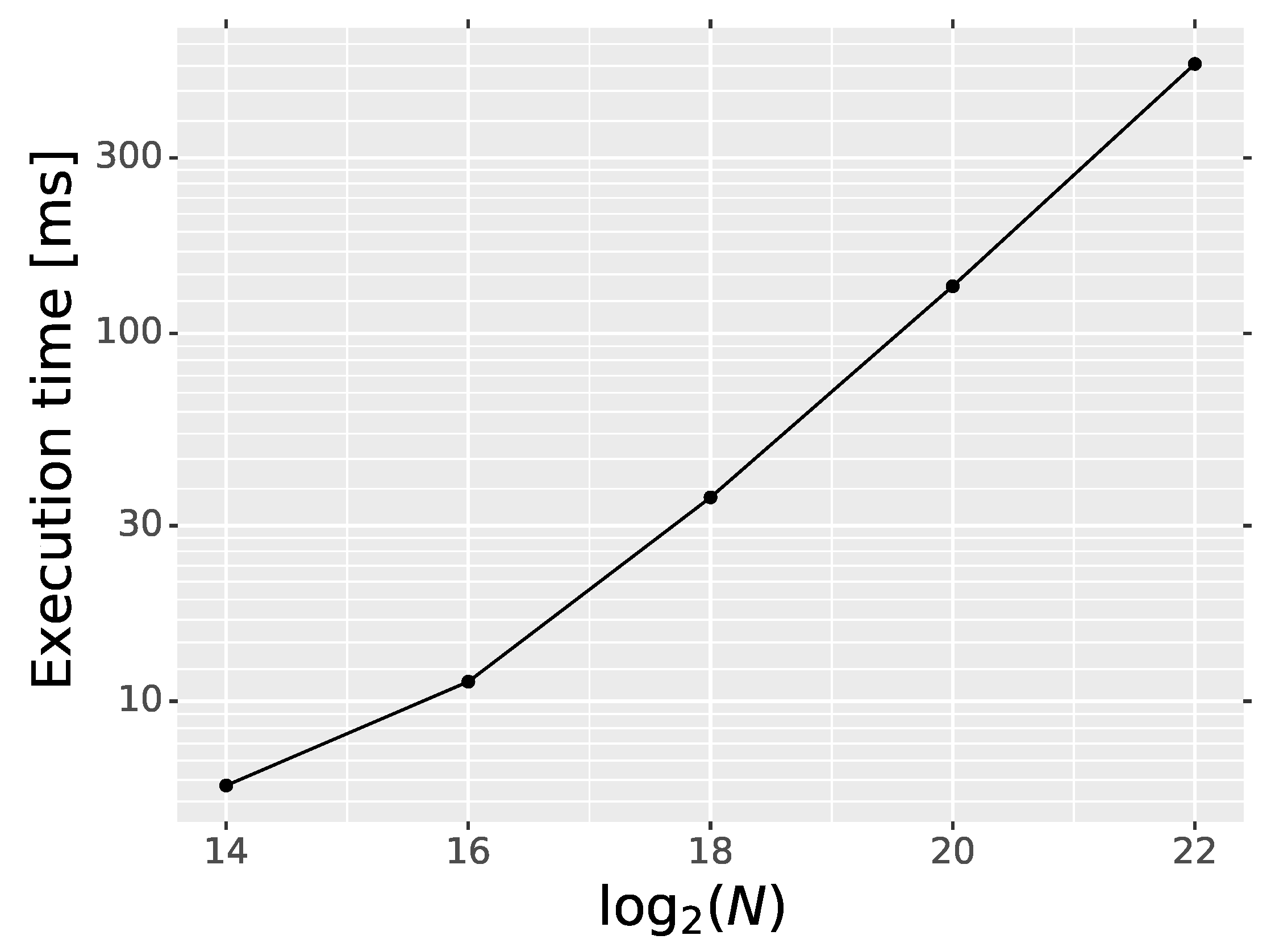
3.4. Computational Complexity

All the experiments were performed in Tensorflow v1.8 [75] environment and Python client, running on a PC with Intel^® Core™ i7-3930K CPU 3.20 GHz and GeForce GTX 1080 Ti. In this setup, the training of the IDCNN detector with the default parameters (see Table 1) takes about six hours on GPU. Regarding the time for inference, we measured only the execution time of operations calculated on GPU, excluding the time required for data image reading and writing. The execution time is summarized in

Table 8. Comparison of average execution time (in miliseconds) of the proposed IDCNN detector and DnCNN method on GPU.

Image Size	${log}_2\mathit{N}$	DnCNN	IDCNN
$128\times 128$	14	5.6	5.9
$256\times 256$	16	11.3	11.3
$512\times 512$	18	36.3	35.8
$1024\times 1024$	20	134.3	134.2
$2048\times 2048$	22	546.3	539.5

. As can be observed, execution time of the proposed IDCNN detector on GPU is similar to DnCNN, which is not surprising because both networks differ only slightly on the last layer. The execution time dependency of the proposed IDCNN on the number of image pixels is depicted in Figure 17. The time required for processing of an image is proportional to the number of pixels N.

4. Conclusions

In this work, we have introduced a switching filter that employs a deep neural network for impulsive noise removal in color images. The performed experiments reveal that the proposed filtering architecture, which operates using a modified version of DnCNN for impulsive pixels detection and adaptive mean filter for their restoration, outperforms or is comparable with the state-of-the-art filters in terms of PSNR, MAE and SSIM_c quality measures.

The proposed IDCNN filter performs well on images contaminated by artificial impulsive noise and also on those affected by real noise process, keeping the undistorted pixels unchanged, without introducing visible artifacts. Apart from the high filtering efficiency, the proposed method is quite fast, and processing of an image of the standard $512\times 512$ size takes about 35 milliseconds on GPU, which enables applying our technique for real time applications. Moreover, the execution time is proportional to the number of pixels, which allows to efficiently process images also in higher resolutions. The unique feature of the introduced switching filter is that it does not require any adjusting parameters, and the same filtering framework can be applied regardless of the image contamination density. In this way, the proposed method can be applied in many denoising scenarios, as no user’s intervention is required. This is a crucial feature of our design, as the methods that deliver good results in terms of objective and also subjective evaluation, need to be tuned, which is mostly difficult and requires experience of the operator.

Future work will be continued in two main directions. The first goal will be the improvement of the efficiency of the noisy pixel replacement using other suitable CNNs. Thus, a combination of the proposed IDCNN for impulse detection and a CNN for noisy pixel restoration will significantly increase the overall performance of noisy image enhancement. The performed experiments indicate that the BDCNN output [72] could be used for the restoration of the detected noisy pixels. Another research direction will be focused on the elaboration of a single network able to combine both the detection and noisy pixel restoration in one processing stage.

References

1. Arnal, J.; Súcar, L.B. Hybrid Filter Based on Fuzzy Techniques for Mixed Noise Reduction in Color Images. Appl. Sci. 2019, 10, 243. [Google Scholar] [CrossRef] [Green Version]
2. Sen, A.P.; Rout, N.K. Removal of High-Density Impulsive Noise in Giemsa Stained Blood Smear Image Using Probabilistic Decision Based Average Trimmed Filter. In Smart Healthcare Analytics in IoT Enabled Environment; Springer International Publishing: Berlin/Heidelberg, Germany, 2020; pp. 127–141. [Google Scholar]
3. Boncelet, C. Image noise models. In Handbook of Image and Video Processing; Bovik, A., Ed.; Academic Press: Cambridge, MA, USA, 2005; pp. 397–410. [Google Scholar]
4. Faraji, H.; MacLean, W. CCD noise removal in digital images. IEEE Trans. Image Process. 2006, 15, 2676–2685. [Google Scholar] [CrossRef] [PubMed]
5. Liu, C.; Szeliski, R.; Bing Kang, S.; Zitnick, C.L.; Freeman, W.T. Automatic Estimation and Removal of Noise from a Single Image. IEEE Trans. Pattern Anal. Mach. Intell. 2008, 30, 299–314. [Google Scholar] [CrossRef] [PubMed] [Green Version]
6. Smolka, B.; Malik, K.; Malik, D. Adaptive rank weighted switching filter for impulsive noise removal in color images. J. Real-Time Image Process. 2012, 10, 289–311. [Google Scholar] [CrossRef] [Green Version]
7. Malinski, L.; Smolka, B. Self-tuning fast adaptive algorithm for impulsive noise suppression in color images. J. Real-Time Image Process. 2019. [Google Scholar] [CrossRef] [Green Version]
8. Plataniotis, K.N.; Venetsanopoulos, A.N. Color Image Filtering. In Color Image Processing and Applications; Digital Signal Processing; Springer: Berlin/Heidelberg, Germnay, 2000; pp. 51–105. [Google Scholar]
9. Smolka, B.; Plataniotis, K.; Venetsanopoulos, A. Chapter Nonlinear Techniques for Color Image Processing. In Nonlinear Signal and Image Processing: Theory, Methods, and Applications; CRC Press: London, UK, 2004; pp. 445–505. [Google Scholar]
10. Phu, M.Q.; Tischer, P.; Wu, H.R. Statistical Analysis of Impulse Noise Model for Color Image Restoration. In Proceedings of the 6th IEEE/ACIS International Conference on Computer and Information Science, Melbourne, Australia, 11–13 July 2007; pp. 425–431. [Google Scholar]
11. Lukac, R.; Smolka, B.; Plataniotis, K.N.; Venetsanopoulos, A.N. Entropy Vector Median Filter. In Pattern Recognition and Image Analysis; Springer: Berlin/Heidelberg, Germany, 2003; pp. 1117–1125. [Google Scholar]
12. Lukac, R.; Smolka, B.; Martin, K.; Plataniotis, K.; Venetsanopoulos, A. Vector filtering for color imaging. IEEE Signal Process. Mag. 2005, 22, 74–86. [Google Scholar] [CrossRef]
13. Lukac, R.; Plataniotis, K. A Taxonomy of Color Image Filtering and Enhancement Solutions. In Advances in Imaging and Electron Physics; Elsevier: Amsterdam, The Netherlands, 2006; Volume 140, pp. 187–264. [Google Scholar]
14. Morillas, S.; Gregori, V.; Sapena, A. Adaptive marginal median filter for colour images. Sensors 2011, 11, 3205–3213. [Google Scholar] [CrossRef] [Green Version]
15. Astola, J.; Haavisto, P.; Neuvo, Y. Vector median filters. Proc. IEEE 1990, 78, 678–689. [Google Scholar] [CrossRef]
16. Lukac, R.; Smolka, B.; Plataniotis, K.; Venetsanopoulos, A. Vector sigma filters for noise detection and removal in color images. J. Vis. Commun. Image Represent. 2006, 17, 1–26. [Google Scholar] [CrossRef]
17. Lukac, R. Adaptive vector median filtering. Pattern Recognit. Lett. 2003, 24, 1889–1899. [Google Scholar] [CrossRef]
18. Celebi, M.E.; Kingravi, H.A.; Aslandogan, Y.A. Nonlinear vector filtering for impulsive noise removal from color images. J. Electron. Imaging 2007, 16, 033008. [Google Scholar] [CrossRef]
19. Morillas, S.; Gregori, V. Robustifying vector median filter. Sensors 2011, 11, 8115–8126. [Google Scholar] [CrossRef] [PubMed]
20. Panetta, K.; Bao, L.; Agaian, S. A New Unified Impulse Noise Removal Algorithm Using a New Reference Sequence-to-Sequence Similarity Detector. IEEE Access 2018, 6, 37225–37236. [Google Scholar] [CrossRef]
21. Chen, J.; Zhan, Y.; Cao, H. Adaptive Sequentially Weighted Median Filter for Image Highly Corrupted by Impulse Noise. IEEE Access 2019, 7, 158545–158556. [Google Scholar] [CrossRef]
22. Elad, M.; Aharon, M. Image Denoising Via Sparse and Redundant Representations Over Learned Dictionaries. IEEE Trans. Image Process. 2006, 15, 3736–3745. [Google Scholar] [CrossRef]
23. Li, X.; Shen, H.; Zhang, L.; Zhang, H.; Yuan, Q.; Yang, G. Recovering Quantitative Remote Sensing Products Contaminated by Thick Clouds and Shadows Using Multitemporal Dictionary Learning. IEEE Trans. Geosci. Remote Sens. 2014, 52, 7086–7098. [Google Scholar]
24. Farouk, R.M.; Khalil, H.A. Image Denoising based on Sparse Representation and Non-Negative Matrix Factorization. Life Sci. J. 2012, 9, 337–341. [Google Scholar]
25. Li, X.; Wang, L.; Cheng, Q.; Wu, P.; Gan, W.; Fang, L. Cloud removal in remote sensing images using nonnegative matrix factorization and error correction. ISPRS J. Photogramm. Remote Sens. 2019, 148, 103–113. [Google Scholar] [CrossRef]
26. Chatzis, V.; Pitas, I. Fuzzy scalar and vector median filters based on fuzzy distances. IEEE Trans. Image Process. 1999, 8, 731–734. [Google Scholar] [CrossRef]
27. Plataniotis, K.; Androutsos, D.; Venetsanopoulos, A. Adaptive fuzzy systems for multichannel signal processing. Proc. IEEE 1999, 87, 1601–1622. [Google Scholar] [CrossRef] [Green Version]
28. Shen, Y.; Barner, K. Fuzzy vector median-based surface smoothing. IEEE Trans. Vis. Comput. Graph. 2004, 10, 252–265. [Google Scholar] [CrossRef] [PubMed]
29. Morillas, S.; Gregori, V.; Peris-Fajarnés, G.; Latorre, P. A New Vector Median Filter Based on Fuzzy Metrics; Lecture Notes in Computer Science; Springer: Berlin/Heidelberg, Germany, 2005; Volume 3656, pp. 81–90. [Google Scholar]
30. Camarena, J.G.; Gregori, V.; Morillas, S.; Sapena, A. Fast detection and removal of impulsive noise using peer groups and fuzzy metrics. J. Vis. Commun. Image Represent. 2008, 19, 20–29. [Google Scholar] [CrossRef]
31. Morillas, S.; Gregori, V.; Hervas, A. Fuzzy Peer Groups for Reducing Mixed Gaussian-Impulse Noise from Color Images. IEEE Trans. Image Process. 2009, 18, 1452–1466. [Google Scholar] [CrossRef]
32. Malinski, L.; Smolka, B. Fast adaptive switching technique of impulsive noise removal in color images. J. Real-Time Image Process. 2019, 16, 1077–1098. [Google Scholar] [CrossRef] [Green Version]
33. Garnett, R.; Huegerich, T.; Chui, C.; He, W. A universal noise removal algorithm with an impulse detector. IEEE Trans. Image Process. 2005, 14, 1747–1754. [Google Scholar] [CrossRef] [PubMed] [Green Version]
34. Deng, Y.; Kenney, C.; Moore, M.; Manjunath, B. Peer group filtering and perceptual color image quantization. In Proceedings of the 1999 IEEE International Symposium on Circuits and Systems, Orlando, FL, USA, 30 May–2 June 1999; Volume 4, pp. 21–24. [Google Scholar]
35. Kenney, C.; Deng, Y.; Manjunath, B.; Hewer, G. Peer group image enhancement. IEEE Trans. Image Process. 2001, 10, 326–334. [Google Scholar] [CrossRef] [PubMed]
36. Malinski, L.; Smolka, B. Fast averaging peer group filter for the impulsive noise removal in color images. J. Real-Time Image Process. 2016, 11, 427–444. [Google Scholar] [CrossRef] [Green Version]
37. Jin, L.; Liu, H.; Xu, X.; Song, E. Quaternion-based color image filtering for impulsive noise suppression. J. Electron. Imaging 2010, 19, 043003. [Google Scholar] [CrossRef]
38. Geng Xin, H.X. Quaternion based switching filter for impulse noise removal in color images. J. Beijing Univ. Aeronaut. Astronaut. 2012, 92, 1181. [Google Scholar]
39. Lin, T.C. Decision-based filter based on SVM and evidence theory for image noise removal. Neural Comput. Appl. 2012, 21, 695–703. [Google Scholar] [CrossRef]
40. Liang, S.; Lu, S.; Chang, J.; Lin, C. A Novel Two-Stage Impulse Noise Removal Technique Based on Neural Networks and Fuzzy Decision. IEEE Trans. Fuzzy Syst. 2008, 16, 863–873. [Google Scholar] [CrossRef]
41. Kaliraj, G.; Baskar, S. An efficient approach for the removal of impulse noise from the corrupted image using neural network based impulse detector. Image Vis. Comput. 2010, 28, 458–466. [Google Scholar] [CrossRef]
42. Nair, M.S.; Shankar, V. Predictive-based adaptive switching median filter for impulse noise removal using neural network-based noise detector. Signal Image Video Process. 2013, 7, 1041–1070. [Google Scholar] [CrossRef]
43. Turkmen, I. The ANN based detector to remove random-valued impulse noise in images. J. Vis. Commun. Image Represent. 2016, 34, 28–36. [Google Scholar] [CrossRef]
44. Lefkimmiatis, S. Non-local Color Image Denoising with Convolutional Neural Networks. In Proceedings of the 2017 IEEE Conference on Computer Vision and Pattern Recognition (CVPR), Honolulu, HI, USA, 21–26 July 2017; pp. 5882–5891. [Google Scholar]
45. Lefkimmiatis, S. Universal Denoising Networks: A Novel CNN Architecture for Image Denoising. In Proceedings of the 2018 IEEE/CVF Conference on Computer Vision and Pattern Recognition, Salt Lake City, UT, USA, 18–22 June 2018; pp. 3204–3213. [Google Scholar]
46. Zhang, K.; Zuo, W.; Zhang, L. FFDNet: Toward a Fast and Flexible Solution for CNN-Based Image Denoising. IEEE Trans. Image Process. 2018, 27, 4608–4622. [Google Scholar] [CrossRef] [PubMed] [Green Version]
47. Fu, B.; Zhao, X.; Li, Y.; Wang, X.; Ren, Y. A convolutional neural networks denoising approach for salt and pepper noise. Multimed. Tools Appl. 2018, 78, 30707–30721. [Google Scholar] [CrossRef] [Green Version]
48. Amaria, Y.; Miyazakia, T.; Koshimuraa, Y.; Yokoyamaa, Y.; Yamamoto, H. A Study on Impulse Noise Reduction Using CNN Learned by Divided Images. In Proceedings of the 6th IIAE International Conference on Industrial Application Engineering, Okinawa, Japan, 20–26 March 2018; pp. 93–100. [Google Scholar]
49. Radlak, K.; Malinski, L.; Smolka, B. Deep learning for impulsive noise removal in color digital images. Procedding of 2019 International Society for Optics and Photonics, Baltimore, MD, USA, 5–8 May 2019; pp. 18–26. [Google Scholar]
50. Chen, J.; Zhang, G.; Xu, S.; Yu, H. A Blind CNN Denoising Model for Random-Valued Impulse Noise. IEEE Access 2019, 7, 124647–124661. [Google Scholar] [CrossRef]
51. Jin, L.; Zhang, W.; Ma, G.; Song, E. Learning deep CNNs for impulse noise removal in images. J. Vis. Commun. Image Represent. 2019, 62, 193–205. [Google Scholar] [CrossRef]
52. Zhang, K.; Zuo, W.; Chen, Y.; Meng, D.; Zhang, L. Beyond a Gaussian Denoiser: Residual Learning of Deep CNN for Image Denoising. IEEE Trans. Image Process. 2017, 26, 3142–3155. [Google Scholar] [CrossRef] [Green Version]
53. Zuo, W.; Zhang, K.; Zhang, L. Convolutional Neural Networks for Image Denoising and Restoration. In Denoising of Photographic Images and Video: Fundamentals, Open Challenges and New Trends; Springer International Publishing: Berlin/Heidelberg, Germany, 2018; pp. 93–123. [Google Scholar]
54. Simonyan, K.; Zisserman, A. Very Deep Convolutional Networks for Large-Scale Image Recognition. In Proceedings of the International Conference on Learning Representations, San Diego, CA, USA, 7–9 May 2015. [Google Scholar]
55. Krizhevsky, A.; Sutskever, I.; Hinton, G.E. ImageNet Classification with Deep Convolutional Neural Networks. In Advances in Neural Information Processing Systems 25; Curran Associates, Inc.: Red Hook, NY, USA, 2012; pp. 1097–1105. [Google Scholar]
56. Ioffe, S.; Szegedy, C. Batch Normalization: Accelerating Deep Network Training by Reducing Internal Covariate Shift. In Proceedings of the 32nd ICML’15 International Conference on International Conference on Machine Learning, Lille, France, 6–11 July 2015; Volume 37, pp. 448–456. [Google Scholar]
57. He, K.; Zhang, X.; Ren, S.; Sun, J. Deep Residual Learning for Image Recognition. In Proceedings of the 2016 IEEE Conference on Computer Vision and Pattern Recognition (CVPR), Las Vegas, NV, USA, 27–30 June 2016; pp. 770–778. [Google Scholar]
58. Zhang, K.; Zuo, W.; Gu, S.; Zhang, L. Learning Deep CNN Denoiser Prior for Image Restoration. In Proceedings of the 2017 IEEE Conference on Computer Vision and Pattern Recognition (CVPR), Honolulu, HI, USA, 21–26 July 2017; pp. 2808–2817. [Google Scholar]
59. Glorot, X.; Bengio, Y. Understanding the difficulty of training deep feedforward neural networks. In Proceedings of the Thirteenth International Conference on Artificial Intelligence and Statistics, Sardinia, Italy, 13–15 May 2010. [Google Scholar]
60. Kingma, D.; Ba, L. Adam: A Method for Stochastic Optimization. In Proceedings of the International Conference on Learning Representations, San Diego, CA, USA, 7–9 May 2015. [Google Scholar]
61. Arbelaez, P.; Maire, M.; Fowlkes, C.; Malik, J. Contour Detection and Hierarchical Image Segmentation. IEEE Trans. Pattern Anal. Mach. Intell. 2011, 33, 898–916. [Google Scholar] [CrossRef] [Green Version]
62. Everingham, M.; Van Gool, L.; Williams, C.K.I.; Winn, J.; Zisserman, A. The PASCAL Visual Object Classes Challenge 2007 (VOC2007) Results. Available online: http://www.pascal-network.org/challenges/VOC/voc2007/workshop/index.html (accessed on 7 May 2020).
63. Kuznetsova, A.; Rom, H.; Alldrin, N.; Uijlings, J.; Krasin, I.; Pont-Tuset, J.; Kamali, S.; Popov, S.; Malloci, M.; Duerig, T.; et al. The Open Images Dataset V4: Unified image classification, object detection, and visual relationship detection at scale. arXiv 2018, arXiv:1811.00982. [Google Scholar] [CrossRef] [Green Version]
64. Jin, L.; Zhu, Z.; Song, E.; Xu, X. An effective vector filter for impulse noise reduction based on adaptive quaternion color distance mechanism. Signal Process. 2019, 155, 334–345. [Google Scholar] [CrossRef]
65. Camarena, J.G.; Gregori, V.; Morillas, S.; Sapena, A. Two-step fuzzy logic-based method for impulse noise detection in colour images. Pattern Recognit. Lett. 2010, 31, 1842–1849. [Google Scholar] [CrossRef]
66. Wu, J.; Tan, C. Random-valued impulse noise removal using fuzzy weighted non-local means. Signal Image Video Process. 2014, 8, 349–355. [Google Scholar] [CrossRef]
67. Schulte, S.; Morillas, S.; Gregori, V.; Kerre, E.E. A New Fuzzy Color Correlated Impulse Noise Reduction Method. IEEE Trans. Image Process. 2007, 16, 2565–2575. [Google Scholar] [CrossRef]
68. Yuan, G.; Ghanem, B. 0TV: A Sparse Optimization Method for Impulse Noise Image Restoration. IEEE Trans. Pattern Anal. Mach. Intell. 2019, 41, 352–364. [Google Scholar] [CrossRef] [Green Version]
69. Delon, J.; Desolneux, A. A Patch-Based Approach for Removing Impulse or Mixed Gaussian-Impulse Noise. SIAM J. Imaging Sci. 2013, 6, 1140–1174. [Google Scholar] [CrossRef]
70. Wang, G.; Liu, Y.; Zhao, T. A quaternion-based switching filter for colour image denoising. Signal Process. 2014, 102, 216–225. [Google Scholar] [CrossRef]
71. Jin, L.; Zhu, Z.; Xu, X.; Li, X. Two-stage quaternion switching vector filter for color impulse noise removal. Signal Process. 2016, 128, 171–185. [Google Scholar] [CrossRef]
72. Abiko, R.; Ikehara, M. Blind Denoising of Mixed Gaussian-impulse Noise by Single CNN. In Proceedings of the 2019 IEEE International Conference on Acoustics, Speech and Signal Processing (ICASSP), Brighton, UK, 12–17 May 2019; pp. 1717–1721. [Google Scholar]
73. Zhou, Y.; Jiao, J.; Huang, H.; Wang, Y.; Wang, J.; Shi, H.; Huang, T. When AWGN-based Denoiser Meets Real Noises. arXiv 2019, arXiv:1904.03485. [Google Scholar]
74. Zhou, W.; Bovik, A.C.; Sheikh, H.R.; Simoncelli, E.P. Image quality assessment: From error visibility to structural similarity. IEEE Trans. Image Process. 2004, 13, 600–612. [Google Scholar]
75. Martín, A.; Agarwal, A.; Barham, P.; Brevdo, E.; Chen, Z.; Citro, C.; Corrado G., S.; Davis, A.; Dean, J.; Devin, M.; et al. TensorFlow: Large-Scale Machine Learning on Heterogeneous Systems. Software. 2015. Available online: tensorflow.org (accessed on 7 May 2020).
Figure 1. A general scheme of a switching filter. Only the pixels identified as corrupted are being restored and the remaining pixels are retained.
Sensors 20 02782 g001
Figure 2. The architecture of the proposed network for impulsive noise detection.
Sensors 20 02782 g002
Figure 3. Training of the proposed Impulse Detection Convolutional Neural Network (IDCNN) detector.example
Sensors 20 02782 g003
Figure 4. Example images from (a) Berkeley segmentation dataset (BSD500) [61] used for training purposes and (b) our test dataset accessible from [36] as supplementary material.
Sensors 20 02782 g004
Figure 5. Exemplary distributions of the IDCNN outputs for the test image contaminated with impulsive noise with intensity ρ = 0.1 and 0.5. For the contamination ρ = 0.1 , 89.59% of pixels are assigned π < 0.1 and 10.14% reaches a value π > 0.9 . For noise intensity ρ = 0.5 , the respective frequencies are 50.20% and 49.44%.
Sensors 20 02782 g005
Figure 6. Repeatability of the training procedure on BSD500 dataset.
Sensors 20 02782 g006
Figure 7. Impact of the patch size p used in the training procedure on the network’s weighted detection accuracy.
Sensors 20 02782 g007
Figure 8. Example images from GoogleV4 and PASCAL VOC2007 datasets [63].
Sensors 20 02782 g008
Figure 9. Impact of the type of dataset used in the training and its size on the average wACC of the proposed IDCNN.
Sensors 20 02782 g009
Figure 10. Impact of the noise density used during training on the final network performance.
Sensors 20 02782 g010
Figure 11. Representative test images from benchmark dataset [36] for which numerical results were calculated.
Sensors 20 02782 g011
Figure 12. Box plots presenting the distributions of the obtained results for the analyzed methods using the test dataset [36].
Sensors 20 02782 g012
Figure 13. Visual comparison of the filtering efficiency using a part of the PEPPERS image ( ρ = 0.4 ).
Sensors 20 02782 g013
Figure 14. Visualization of the denoising efficiency of the proposed IDCNNG in comparison to the ideal impulse detector, which correctly identifies all impulses in the analyzed image ( ρ = 0.4 ). The right column shows the difference between the restored and clean image.
Sensors 20 02782 g014
Figure 15. Denoising result of the proposed IDCNN filter on real noisy images: a part of an image of the fresco “The Condemned in Hell” by Luca Signorelli (top) and cDNA image (bottom). Detected impulses are annotated using cyan color.
Sensors 20 02782 g015
Figure 16. Diagrams that show what portion of the MAE error was caused by the improper decision of the used filter from classification perspective. These diagrams were obtained for the PEPPERS image ( ρ = 0.4).
Sensors 20 02782 g016
Figure 17. Execution time dependency of the IDCNN on the number of image pixels N.
Sensors 20 02782 g017