The Effect of Treadmill Walking on Gait and Upper Trunk through Linear and Nonlinear Analysis Methods


Abstract
1. Introduction
2. Methods
2.1. Participants
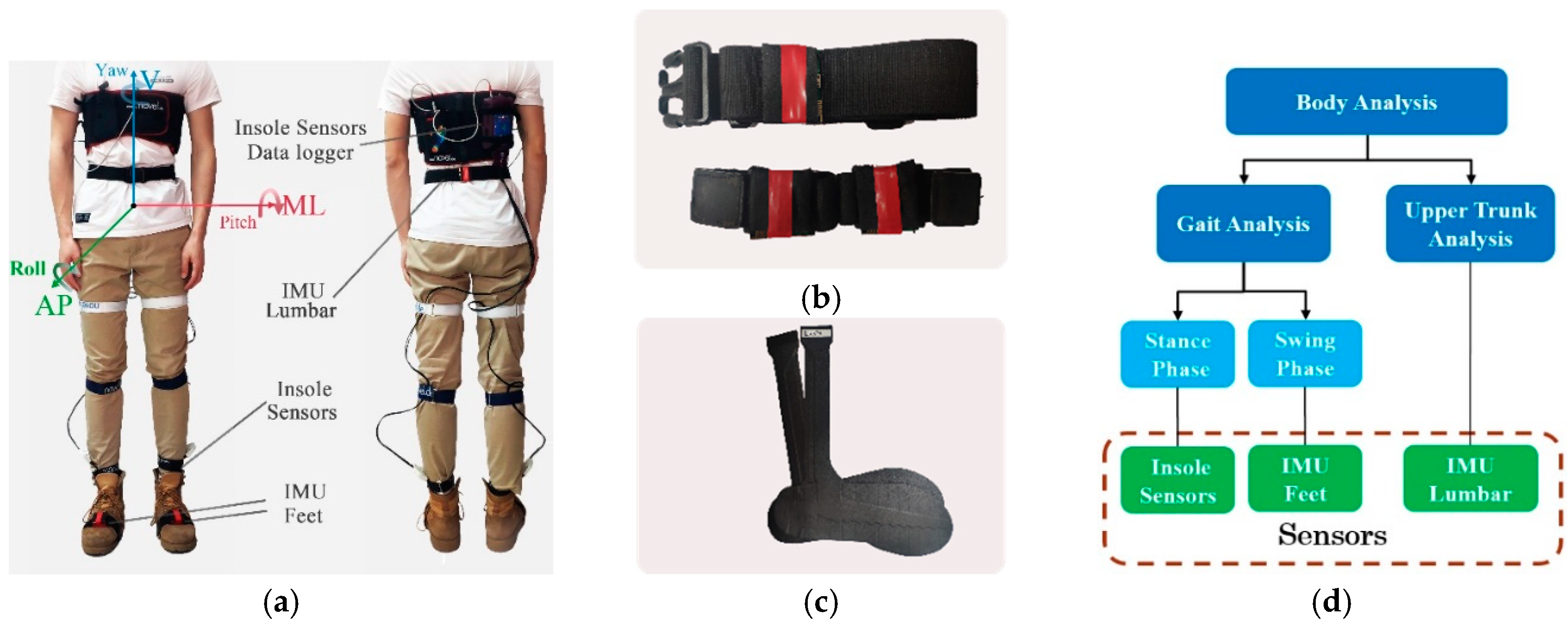
2.2. Apparatus
2.3. Experimental Protocol
2.4. Linear Features
2.5. Nonlinear Features
2.5.1. Sample Entropy
2.5.2. Maximal Lyapunov Exponent
2.5.3. Fractal Dynamic
2.6. Statistical Analysis
3. Results
3.1. Gait Analysis Result
3.2. Upper Trunk Analysis Result
4. Discussion
4.1. Difference between Treadmill and Overground Walking
4.2. Correlation between Gait and Upper Trunk Features
4.3. Technical Issues
5. Conclusions
Author Contributions
Funding
Acknowledgments
Conflicts of Interest
References
- Bello, O.; Marquez, G.; Camblor, M.; Fernandez-Del-Olmo, M. Mechanisms involved in treadmill walking improvements in Parkinson’s disease. Gait Posture 2010, 32, 118–123. [Google Scholar] [CrossRef] [PubMed]
- Mehrholz, J.; Pohl, M.; Elsner, B. Treadmill training and body weight support for walking after stroke. Stroke 2014, 45, E76–E77. [Google Scholar]
- Hicks, A.L.; Ginis, K.A. Treadmill training after spinal cord injury: It’s not just about the walking. J. Rehabil. Res. Dev. 2008, 45, 241–248. [Google Scholar] [CrossRef] [PubMed]
- Lee, S.J.; Hidler, J. Biomechanics of overground vs. treadmill walking in healthy individuals. J. Appl. Physiol. 2008, 104, 747–755. [Google Scholar] [CrossRef] [PubMed]
- Murray, M.P.; Spurr, G.B.; Sepic, S.B.; Gardner, G.M.; Mollinger, L.A. Treadmill vs floor walking: Kinematics, electromyogram, and heart rate. J. Appl. Physiol. 1985, 59, 87–91. [Google Scholar] [CrossRef]
- Isacson, J.; Gransberg, L.; Knutsson, E. Three-dimensional electrogoniometric gait recording. J. Biomech. 1986, 19, 627–635. [Google Scholar] [CrossRef]
- Nymark, J.R.; Balmer, S.J.; Melis, E.H.; Lemair, E.D.; Millar, S. Electromyographic and kinematic nondisabled gait differences at extremely slow overground and treadmill walking speeds. J. Rehabil. Res. Dev. 2005, 42, 523–534. [Google Scholar] [CrossRef]
- Fukuchi, C.A.; Fukuchi, R.K.; Duarte, M. A public dataset of overground and treadmill walking kinematics and kinetics in healthy individuals. Multidiscip. Sci. 2018, 6, e4640. [Google Scholar] [CrossRef]
- White, S.C.; Yack, H.J.; Tucker, C.A.; Lin, H.Y. Comparison of vertical ground reaction forces during overground and treadmill walking. Med. Sci. Sports Exerc. 1998, 30, 1537–1542. [Google Scholar] [CrossRef] [PubMed]
- Riley, P.O.; Paolini, G.; Della Croce, U.; Paylo, K.W.; Kerrigan, D.C. A kinematic and kinetic comparison of overground and treadmill walking in healthy subjects. Gait Posture 2007, 26, 17–24. [Google Scholar] [CrossRef] [PubMed]
- Pearce, M.E.; Cunningham, D.A.; Donner, A.P.; Rechnitzer, P.A.; Fullerton, G.M.; Howard, J.H. Energy cost of treadmill and floor walking at selfselected paces. Eur. J. Phys. 1983, 52, 115–119. [Google Scholar]
- Watt, J.R.; Franz, J.R.; Jackson, K.; Dicharry, J.; Riley, P.O.; Kerrigan, D.C. A three dimensional kinematic and kinetic comparison of overground and treadmill walking in healthy elderly subjects. Clin. Biomech. 2010, 25, 444–449. [Google Scholar] [CrossRef] [PubMed]
- Grieco, J.C.; Gouelle, A.; Weeber, E.J. Identification of spatiotemporal gait parameters and pressure-related characteristics in children with Angelman syndrome: A pilot study. J. Appl. Res. Intellect. Disabil. 2018, 31, 1219–1224. [Google Scholar] [CrossRef] [PubMed]
- Deborah, J.; Julie, N. Fallers with Parkinson’s disease exhibit restrictive trunk control during walking. Gait Posture 2018, 65, 246–250. [Google Scholar]
- Samira, A.; Nariman, S.; Christine, W.; Tony, S. Sample Entropy of Human Gait Center of Pressure Displacement: A Systematic Methodological Analysis. Entropy 2018, 20, 579. [Google Scholar]
- Schulz, B.W. A new measure of trip risk integrating minimum foot clearance and dynamic stability across the swing phase of gait. J. Biomech. 2017, 55, 107–112. [Google Scholar] [CrossRef]
- Rosenblatt, N.J.; Bauer, A.; Grabiner, M.D. Relating minimum toe clearance to prospective, self-reported, trip-related stumbles in the community. Prosthet. Orthot. Int. 2017, 41, 387–392. [Google Scholar] [CrossRef] [PubMed]
- Dadashi, F.; Mariani, B.; Rochat, S.; Bula, C.J.; Santos-Eggimann, B.; Aminian, K. Gait and Foot Clearance Parameters Obtained Using Shoe-Worn Inertial Sensors in a Large-Population Sample of Older Adults. Sensors 2014, 14, 443–457. [Google Scholar] [CrossRef] [PubMed]
- Arami, A.; Saint Raymond, N.; Aminian, K. An Accurate Wearable Foot Clearance Estimation System: Toward a Real-Time Measurement System. IEEE Sens. J. 2017, 17, 2542–2549. [Google Scholar] [CrossRef]
- Dingwell, J.B.; Cusumano, J.P.; Cavanagh, P.R.; Sternad, D. Local dynamic stability versus kinematic variability of continuous overground and treadmill walking. J. Biomech. Eng. 2001, 123, 27–32. [Google Scholar] [CrossRef]
- Terrier, P.; Deriaz, O. Kinematic variability, fractal dynamics and local dynamic stability of treadmill walking. J. Neuroeng. Rehabil. 2011, 8, 12. [Google Scholar] [CrossRef] [PubMed]
- Terrier, P.; Reynard, F. Effect of age on the variability and stability of gait: A cross-sectional treadmill study in healthy individuals between 20 and 69 years of age. Gait Posture 2015, 41, 170–174. [Google Scholar] [CrossRef] [PubMed]
- Kobayashi, H.; Kakihana, W.; Kimura, T. Combined effects of age and gender on gait symmetry and regularity assessed by autocorrelation of trunk acceleration. J. Neuroeng. Rehabil. 2014, 11, 109. [Google Scholar] [CrossRef] [PubMed]
- Madgwick, S.O.H.; Harrison, A.J.L.; Vaidyanathan, A. Estimation of IMU and MARG orientation using a gradient descent algorithm. In Proceedings of the IEEE International Conference on Rehabilitation Robotics, Zurich, Switzerland, 27 June–1 July 2011. [Google Scholar]
- Menz, H.B.; Lord, S.R.; Fitzpatrick, R.C. Acceleration patterns of the head and pelvis when walking on level and irregular surfaces. Gait Posture 2003, 18, 35–46. [Google Scholar] [CrossRef]
- Nishiguchi, S.; Yamada, M.; Nagai, K.; Mori, S.; Kajiwara, Y.; Sonoda, T.; Yoshimura, K.; Yoshitomi, H.; Ito, H.; Okamoto, K.; et al. Reliability and validity of gait analysis by android-based smartphone. Telemed. J. E-Health 2012, 18, 292–296. [Google Scholar] [CrossRef] [PubMed]
- Taylor & Francis Group. Nonlinear Analysis for Human Movement Variability; CRC Press: Boca Raton, FL, USA, 2016. [Google Scholar]
- Yentes, J.M.; Hunt, N.; Schmid, K.K.; Kaipust, J.P.; McGrath, D.; Stergiou, N. The appropriate use of approximate entropy and sample entropy with short data sets. Annals Biomed. Eng. 2013, 41, 349–365. [Google Scholar] [CrossRef] [PubMed]
- Pincus, S.M.; Goldberger, A.L. Physiological time-series analysis: What does regularity quantify? Am. J. Physiol. 1994, 266, H1643–H1656. [Google Scholar] [CrossRef] [PubMed]
- Richman, J.S.; Moorman, J.R. Physiological time series analysis using approximate entropy and sample entropy. Am. J. Physiol. 2000, 278, H2039–H2049. [Google Scholar] [CrossRef] [PubMed]
- Dingwell, J.B.; Cusumano, J.P. Nonlinear time series analysis of normal and pathological human walking. Chaos 2000, 10, 848–863. [Google Scholar] [CrossRef] [PubMed]
- Wolf, A.; Swift, J.B.; Swinney, H.L.; Vastano, J.A. Determining Lyapunov exponents from a time series. Phys. D Nonlinear Phenom. 1985, 16, 285–317. [Google Scholar] [CrossRef]
- Rosenstein, M.T.; Collins, J.J.; De Luca, C.J. A practical method for calculating largest Lyapunov exponents from small data sets. Phys. D Nonlinear Phenom. 1993, 65, 117–134. [Google Scholar] [CrossRef]
- Abarbanel, H.D.I. Analysis of Observed Chaotic Data; Springer: New York, NY, USA, 1996. [Google Scholar]
- Nakagawa, S.; Cuthill, I.C. Effect size, confidence interval and statistical significance: A practical guide for biologists. Biol. Rev. 2007, 82, 591–605. [Google Scholar] [CrossRef] [PubMed]
- Alvaro, M.H.; Begonya, G.Z.; Amaia, M.Z. Gait Analysis Methods: An Overview of Wearable and Non-Wearable Systems, Highlighting Clinical Applications. Sensors 2014, 14, 3362–3394. [Google Scholar]
- Davide, M.; Mosè, C.; Aitor, M.F. The effect of treadmill and overground walking on preferred walking speed and gait kinematics in healthy, physically active. Eur. J. Appl. Physiol. 2017, 117, 1833–1843. [Google Scholar]
- Davis, A.M.; Galna, B.; Murphy, A.T.; Williams, C.M.; Haines, T.P. Effect of footwear on minimum foot clearance, heel slippage and spatiotemporal measures of gait in older women. Gait Posture 2016, 44, 43–47. [Google Scholar] [CrossRef] [PubMed]
- Hong, S.K.; Park, S.H.; Shin, S.R.; Lee, D.G.; Lee, S.H.; Jung, S.H.; Pyo, S.H.; Lee, K.B.; Lee, G.C. Comparison of spatio-temporal gait parameters according to shoe types in chronic stroke survivors: A preliminary study. Phys. Therapy Rehabil. Sci. 2018, 7, 23–28. [Google Scholar] [CrossRef]


| Gait Variable | Authors | Results | References |
|---|---|---|---|
| Spatiotemporal parameters | Lee et al. | Young and elderly people both had longer stance time under OW condition. | [4] |
| Watt et al. | Stride time and length of OW were greater than TW. | [12] | |
| COP | Grieco et al. | A less efficient and consistent COP pathway was shown in angelman syndrome children than healthy children. | [13] |
| Deborah et al. | COP velocity in anterior-posterior direction of healthy older adults was larger than those with Parkinson diseases. | [14] | |
| Samira et al. | Sample entropy of COP could maintain the directional difference between treadmill walking only and dual-task condition across variant parameter values. | [15] | |
| Foot clearance | Dadashi et al. | Foot clearance could characterize the risky gait pattern through analyzing the dataset from 1400 participants. | [18] |
| Arami et al. | An accurate wearable foot clearance estimation system with infrared distance meter sensors and inertial measurement unit was designed to provide a real-time estimation of foot height and orientation. | [19] |
| Linear Features | Data Source | |
|---|---|---|
| Spatiotemporal parameters | Stride length | Insole sensors |
| Stride time | Insole sensors | |
| CV of stride time | Insole sensors | |
| Gait features of swing phase | RMS of acceleration in V direction | IMU Feet |
| Gait features of stance phase (COP) | COP efficiency | Insole sensors |
| C-M distance | Insole sensors | |
| Std ML-CISP | Insole sensors | |
| Std AP-CISP | Insole sensors | |
| Upper trunk features | RMS of movement degree in pitch direction | IMU Lumbar |
| RMS of movement degree in roll direction | IMU Lumbar | |
| RMS of movement degree in yaw direction | IMU Lumbar | |
| RMS of acceleration in ML direction | IMU Lumbar | |
| RMS of acceleration in V direction | IMU Lumbar | |
| RMS of acceleration in AP direction | IMU Lumbar | |
| Nonlinear Features | Data Source | |
|---|---|---|
| Spatiotemporal parameters | Scaling exponent α of stride intervals (DFA) | Insole sensors |
| Gait features of swing phase | Maximal Lyapunov exponent λ of foot acceleration in V direction | IMU Feet |
| Sample entropy of foot acceleration in V direction | IMU Feet | |
| Gait features of stance phase (COP) | Maximal Lyapunov exponent λ of COP position in ML direction | Insole sensors |
| Maximal Lyapunov exponent λ of COP position in AP direction | Insole sensors | |
| Sample entropy of COP position in ML direction | Insole sensors | |
| Sample entropy of COP position in AP direction | Insole sensors | |
| Upper trunk features | Maximal Lyapunov exponent λ of lumbar acceleration in ML direction | IMU Lumbar |
| Maximal Lyapunov exponent λ of lumbar acceleration in V direction | IMU Lumbar | |
| Maximal Lyapunov exponent λ of lumbar acceleration in AP direction | IMU Lumbar | |
| Upper trunk features | Sample entropy of lumbar acceleration in ML direction | IMU Lumbar |
| Sample entropy of lumbar acceleration in V direction | IMU Lumbar | |
| Sample entropy of lumbar acceleration in AP direction | IMU Lumbar | |
| OW | TW | Effect Size | T-test | ||||
|---|---|---|---|---|---|---|---|
| N = 8 | Mean ± Std | CI | Mean ± Std | CI | OW − TW | Norm. | p |
| Stride length (m) | 1.391 ± 0.112 | 1.313 − 1.469 | 1.341 ± 0.103 | 1.270 − 1.412 | 0.050 | 0.464 | 0.028 |
| Stride time (s) | 1.062 ± 0.049 | 1.028 − 1.096 | 1.031 ± 0.052 | 0.994 − 1.067 | 0.032 | 0.626 | 0.005 |
| CV of stride time (%) | 1.877 ± 0.432 | 1.577 − 2.177 | 1.782 ± 0.344 | 1.544 − 2.021 | 0.095 | 0.242 | 0.626 |
| α (DFA) | 0.819 ± 0.150 | 0.716 − 0.923 | 0.663 ± 0.101 | 0.593 − 0.733 | 0.156 | 1.223 | 0.016 |
| OW | TW | Effect Size | T-test | ||||
|---|---|---|---|---|---|---|---|
| N = 8 | Mean ± Std | CI | Mean ± Std | CI | OW − TW | Norm. | p |
| RMS of acceleration | 2.021 ± 0.438 | 1.717 − 2.324 | 1.534 ± 0.392 | 1.262 − 1.805 | 0.487 | 1.172 | 0.009 |
| λ | 0.024 ± 0.005 | 0.021 − 0.028 | 0.023 ± 0.005 | 0.019 − 0.026 | 0.002 | 0.346 | 0.495 |
| Sample entropy | 0.115 ± 0.016 | 0.104 − 0.126 | 0.341 ± 0.045 | 0.310 − 0.372 | −0.226 | −6.715 | 0.000 |
| OW | TW | Effect Size | T-test | ||||
|---|---|---|---|---|---|---|---|
| N = 8 | Mean ± Std | CI | Mean ± Std | CI | OW − TW | Norm. | p |
| COP efficiency (%) | 96.406 ± 0.980 | 95.726 − 97.085 | 95.337 ± 1.811 | 94.083 − 96.592 | 1.068 | 0.734 | 0.029 |
| C-M distance (mm) | 34.125 ±7.453 | 28.960 − 39.290 | 31.375 ± 4.658 | 28.147 − 34.603 | 2.750 | 0.442 | 0.332 |
| Std ML-CISP (mm) | 1.508 ± 0.318 | 1.287 − 1.728 | 1.481 ± 0.350 | 1.238 − 1.723 | 0.027 | 0.080 | 0.835 |
| Std AP-CISP (mm) | 3.207 ± 0.409 | 2.923 − 3.490 | 2.994 ± 0.487 | 2.656 − 3.332 | 0.213 | 0.473 | 0.211 |
| λ-ML | 0.006 ± 0.007 | 0.001 − 0.012 | 0.013 ± 0.010 | 0.006 − 0.020 | −0.006 | −0.733 | 0.141 |
| λ-AP | −0.006 ± 0.012 | −0.015 − 0.002 | −0.018 ± 0.016 | −0.029 − −0.007 | 0.012 | 0.858 | 0.042 |
| Sample entropy-ML | 0.062 ± 0.006 | 0.058 − 0.066 | 0.061 ± 0.006 | 0.057 − 0.065 | 0.001 | 0.145 | 0.585 |
| Sample entropy-AP | 0.064 ± 0.006 | 0.060 − 0.069 | 0.061 ± 0.006 | 0.057 − 0.065 | 0.003 | 0.474 | 0.387 |
| OW | TW | Effect Size | T-test | ||||
|---|---|---|---|---|---|---|---|
| N = 8 | Mean ± Std | CI | Mean ± Std | CI | OW − TW | Norm. | p |
| RMS of pitch degree (°) | 0.909 ± 0.308 | 0.696 − 1.123 | 0.936 ± 0.243 | 0.767 − 1.104 | −0.026 | −0.095 | 0.623 |
| RMS of roll degree (°) | 0.947 ± 0.421 | 0.655 − 1.238 | 0.920 ± 0.207 | 0.776 − 1.063 | 0.027 | 0.082 | 0.785 |
| RMS of yaw degree (°) | 1.649 ± 0.401 | 1.370 − 1.927 | 1.764 ± 0.478 | 1.433 − 2.095 | −0.116 | −0.263 | 0.339 |
| RMS of acceleration (ML) | 0.413 ± 0.122 | 0.328 − 0.498 | 0.468 ± 0.144 | 0.369 − 0.568 | −0.056 | −0.416 | 0.215 |
| RMS of acceleration (V) | 0.840 ± 0.212 | 0.693 − 0.987 | 0.650 ± 0.216 | 0.500 − 0.799 | 0.190 | 0.887 | 0.008 |
| RMS of acceleration (AP) | 1.267 ± 0.182 | 1.140 − 1.393 | 1.059 ± 0.243 | 0.891 − 1.228 | 0.207 | 0.965 | 0.014 |
| λ-ML | 0.044 ± 0.013 | 0.035 − 0.053 | 0.026 ± 0.011 | 0.019 − 0.034 | 0.018 | 1.448 | 0.043 |
| λ-V | 0.011 ± 0.009 | 0.005 − 0.018 | 0.011 ± 0.009 | 0.005 − 0.018 | 0.000 | 0.010 | 0.983 |
| λ-AP | 0.009 ± 0.006 | 0.005 − 0.013 | 0.005 ± 0.007 | 0.001 − 0.010 | 0.004 | 0.576 | 0.323 |
| Sample entropy-ML | 0.581 ± 0.151 | 0.476 − 0.686 | 0.689 ± 0.219 | 0.537 − 0.841 | −0.107 | −0.571 | 0.313 |
| Sample entropy-V | 0.376 ± 0.111 | 0.299 − 0.453 | 0.515 ± 0.141 | 0.418 − 0.613 | −0.139 | −1.098 | 0.086 |
| Sample entropy-AP | 0.390 ± 0.045 | 0.358 − 0.421 | 0.401 ± 0.078 | 0.347 − 0.455 | −0.012 | −0.181 | 0.759 |
| N = 8 | Gait | ||||||||
|---|---|---|---|---|---|---|---|---|---|
| Walking Speed | Stride Time | COP Path Efficiency | λ-ML | ||||||
| OW | TW | OW | TW | OW | TW | OW | TW | ||
| Upper Trunk | RMS of pitch degree | −0.313 | −0.225 | 0.295 | 0.234 | −0.779 * | −0.152 | 0.212 | 0.054 |
| RMS of roll degree | −0.881 ** | −0.667 | 0.813 * | 0.450 | −0.754 * | −0.457 | −0.475 | 0.383 | |
| RMS of yaw degree | −0.452 | −0.733 * | 0.648 | 0.578 | −0.323 | −0.659 | −0.334 | 0.539 | |
| Sample entropy-ML | −0.659 | −0.191 | 0.900 ** | 0.044 | −0.379 | −0.390 | −0.718 * | 0.417 | |
| Sample entropy-V | −0.549 | 0.012 | 0.835 ** | −0.460 | −0.164 | 0.050 | −0.813* | 0.346 | |
| Sample entropy-AP | −0.882 ** | 0.052 | 0.744 * | −0.306 | −0.571 | −0.098 | −0.427 | 0.184 | |
| RMS of acceleration-ML | −0.841 ** | −0.604 | 0.632 | 0.353 | −0.606 | −0.242 | −0.290 | 0.183 | |
| RMS of acceleration-V | −0.852 ** | −0.680 | 0.600 | 0.672 | −0.787 * | −0.670 | −0.162 | 0.366 | |
| RMS of acceleration-AP | −0.472 | −0.197 | 0.242 | 0.221 | 0.047 | −0.165 | −0.244 | 0.178 | |
© 2019 by the authors. Licensee MDPI, Basel, Switzerland. This article is an open access article distributed under the terms and conditions of the Creative Commons Attribution (CC BY) license (http://creativecommons.org/licenses/by/4.0/).
Share and Cite
Shi, L.; Duan, F.; Yang, Y.; Sun, Z. The Effect of Treadmill Walking on Gait and Upper Trunk through Linear and Nonlinear Analysis Methods. Sensors 2019, 19, 2204. https://doi.org/10.3390/s19092204
Shi L, Duan F, Yang Y, Sun Z. The Effect of Treadmill Walking on Gait and Upper Trunk through Linear and Nonlinear Analysis Methods. Sensors. 2019; 19(9):2204. https://doi.org/10.3390/s19092204
Chicago/Turabian StyleShi, Liang, Feng Duan, Yikang Yang, and Zhe Sun. 2019. "The Effect of Treadmill Walking on Gait and Upper Trunk through Linear and Nonlinear Analysis Methods" Sensors 19, no. 9: 2204. https://doi.org/10.3390/s19092204
APA StyleShi, L., Duan, F., Yang, Y., & Sun, Z. (2019). The Effect of Treadmill Walking on Gait and Upper Trunk through Linear and Nonlinear Analysis Methods. Sensors, 19(9), 2204. https://doi.org/10.3390/s19092204