Adaptive Selection of Truncation Radius in Calderon’s Method for Direct Image Reconstruction in Electrical Capacitance Tomography †


Abstract
1. Introduction
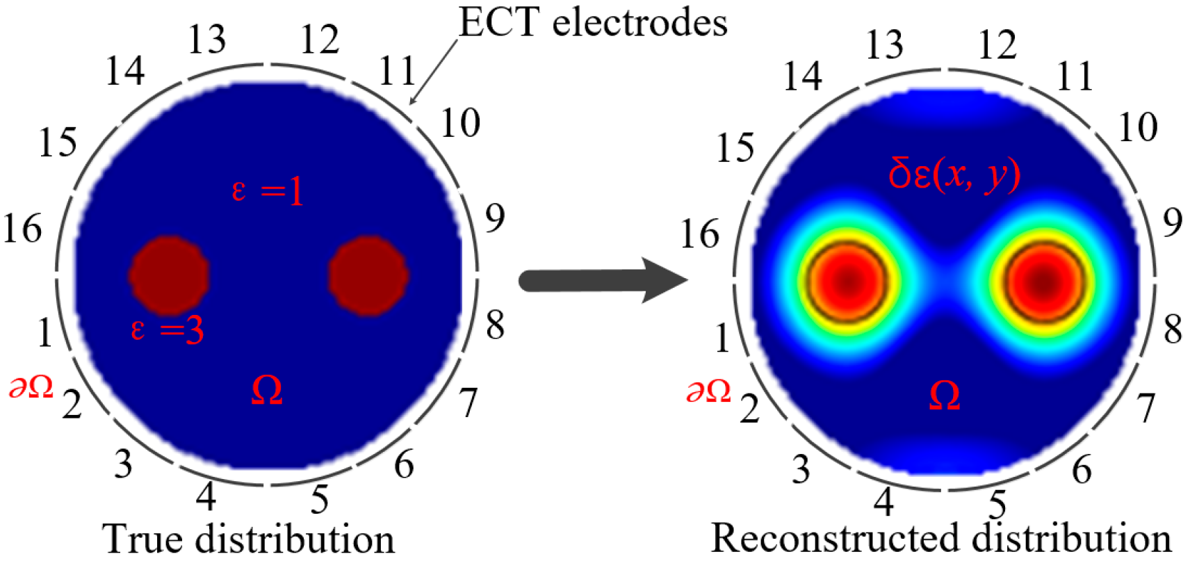
2. Calderon’s Method for Direct Image Reconstruction in ECT
3. Adaptive Selection of Truncation Radius
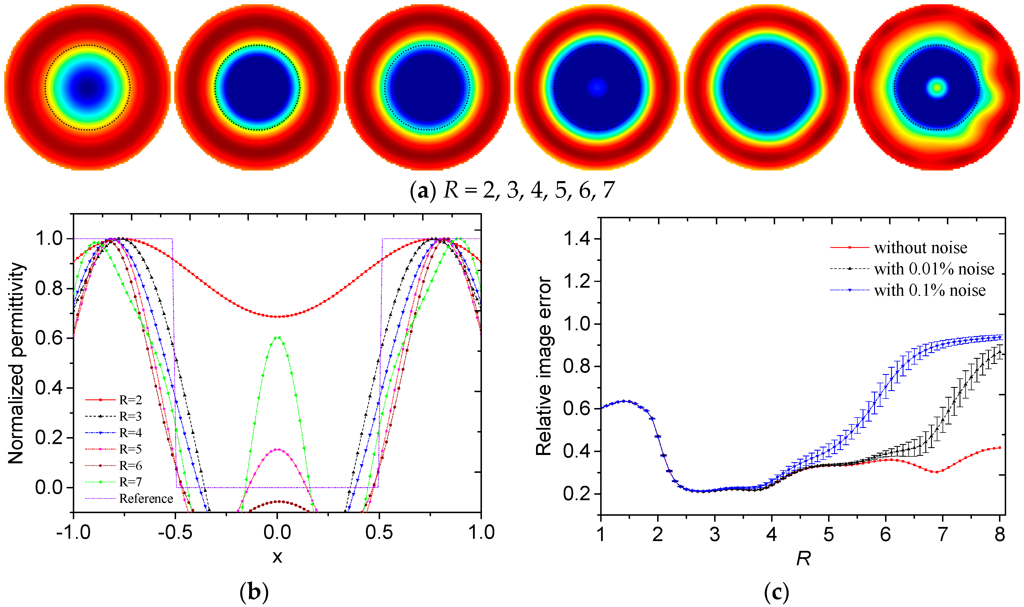
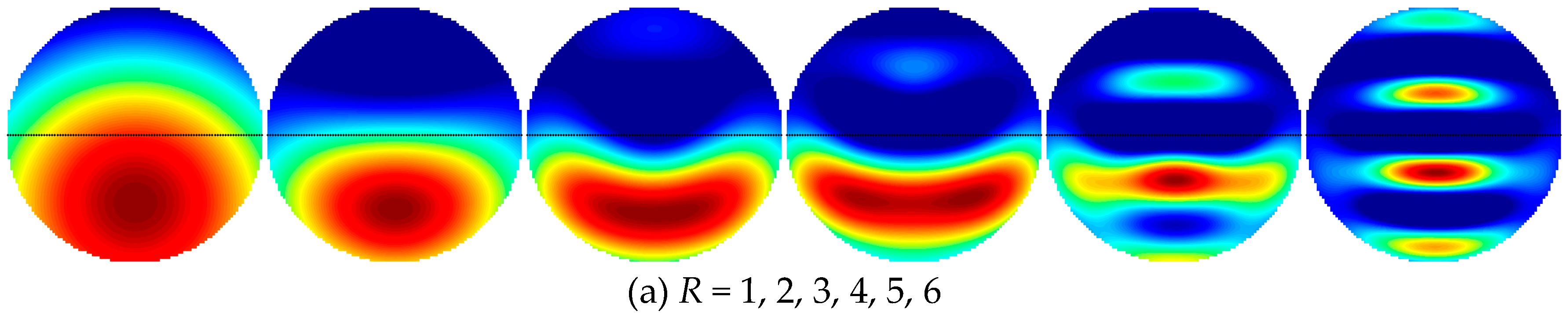
3.1. Influence of the Truncation Radius on Reconstructed Results in Spatial Domain
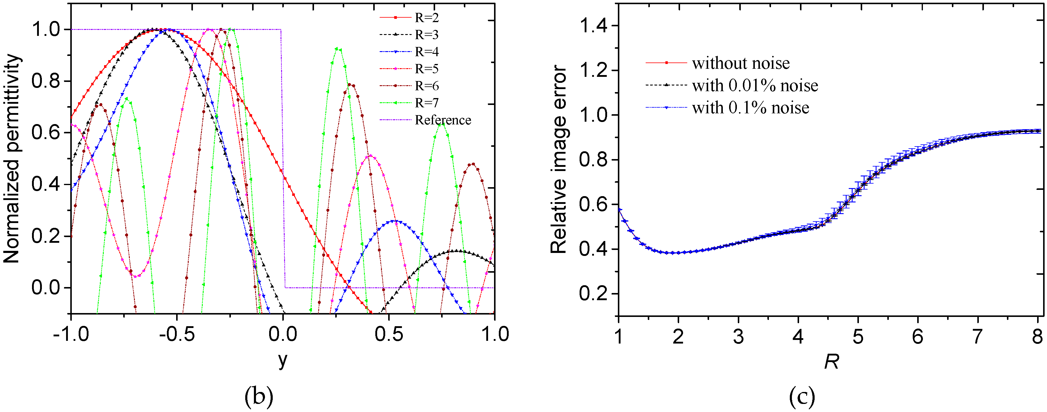
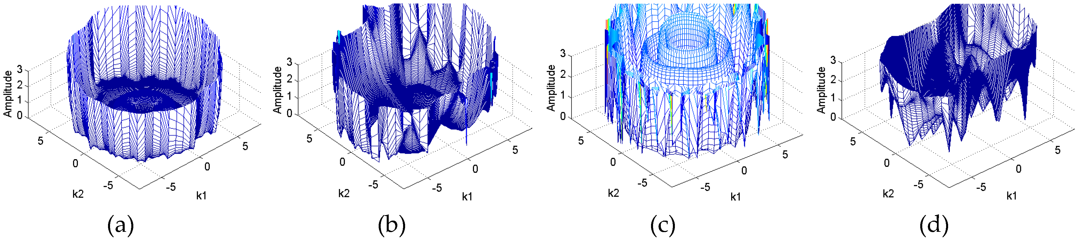
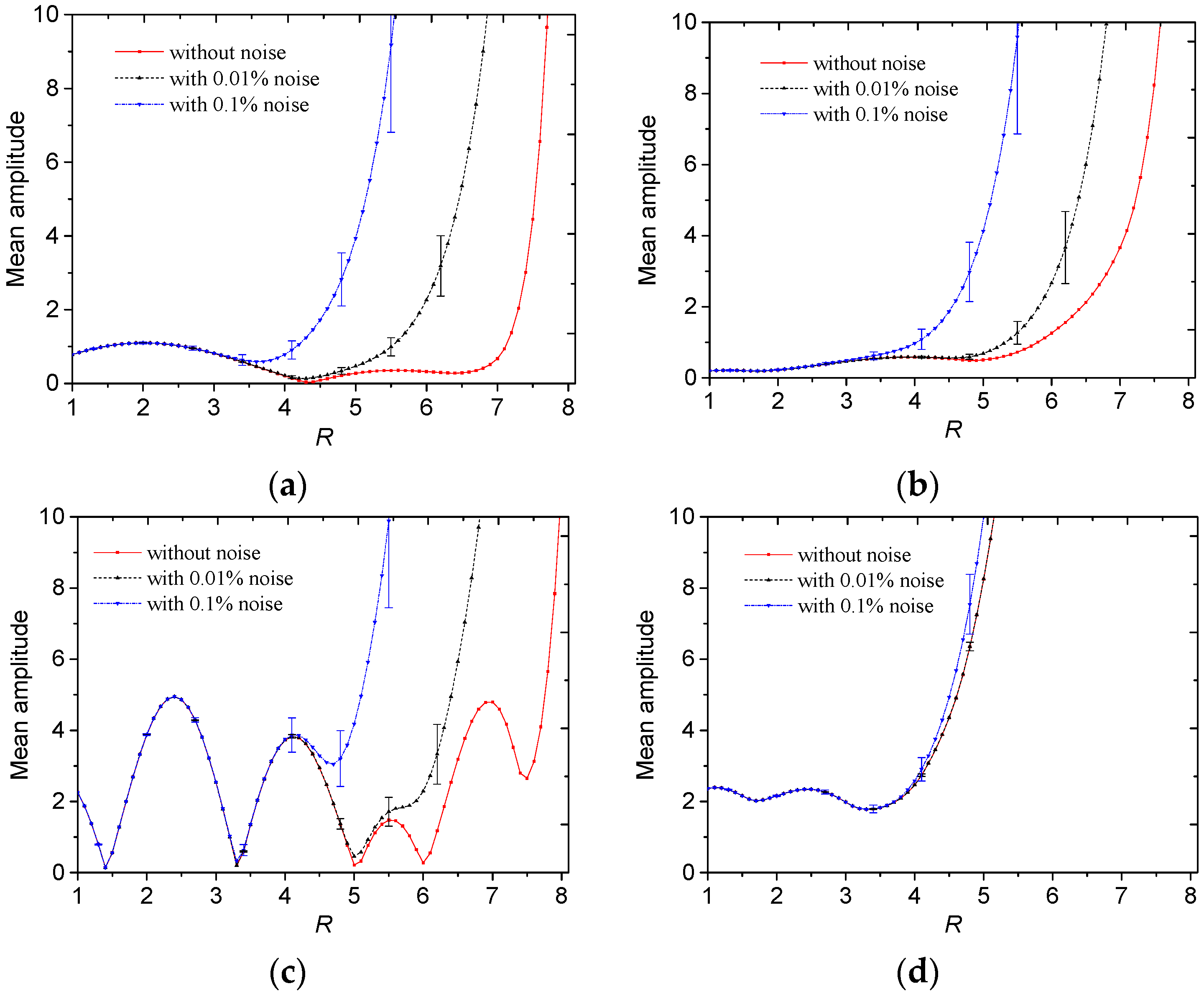
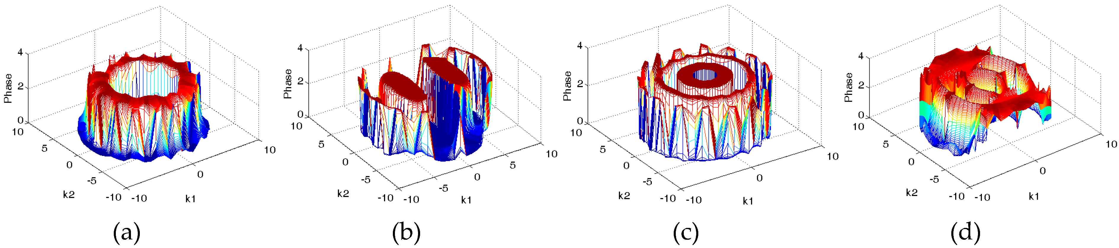
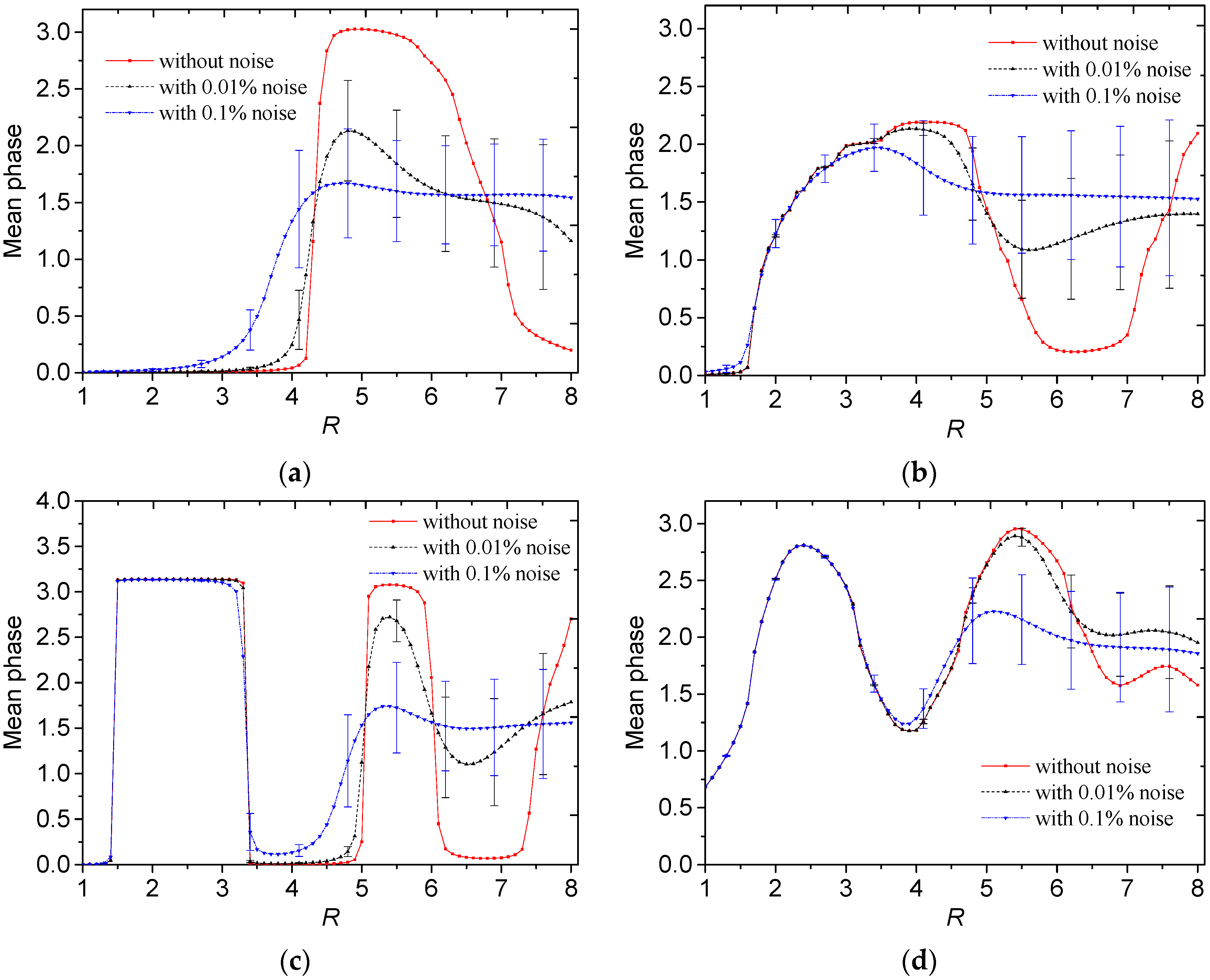
3.2. Influence of the Truncation Radius on Scattering Transform in the Frequency Domain
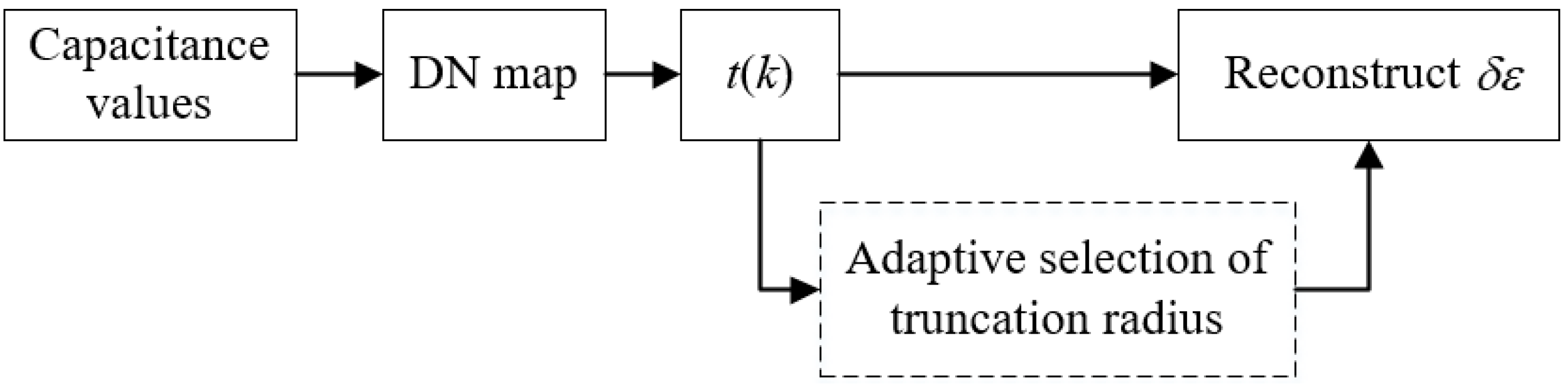
3.3. Adaptive Selection of the Truncation Radius
4. Experimental Results
5. Conclusions
- (1)
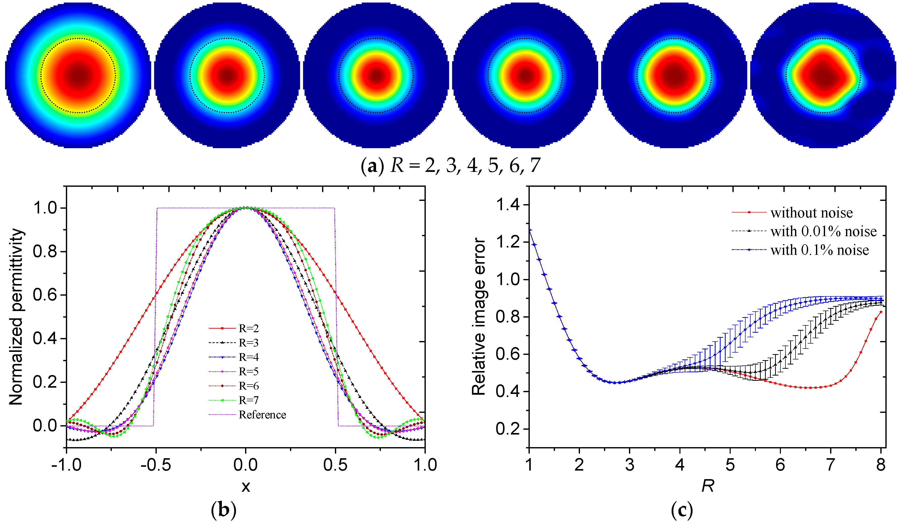
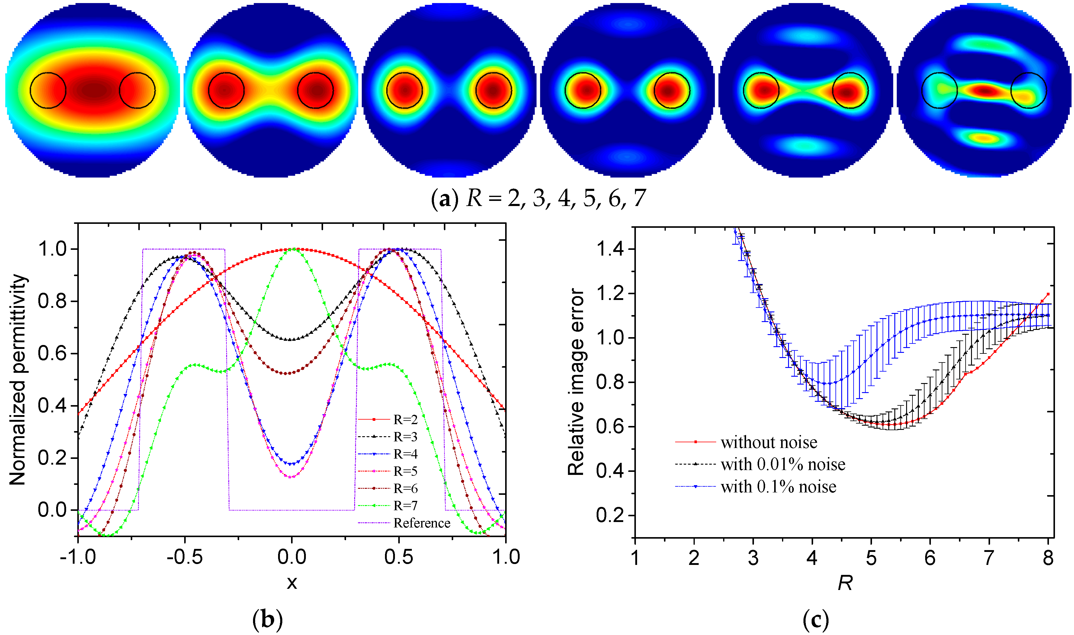
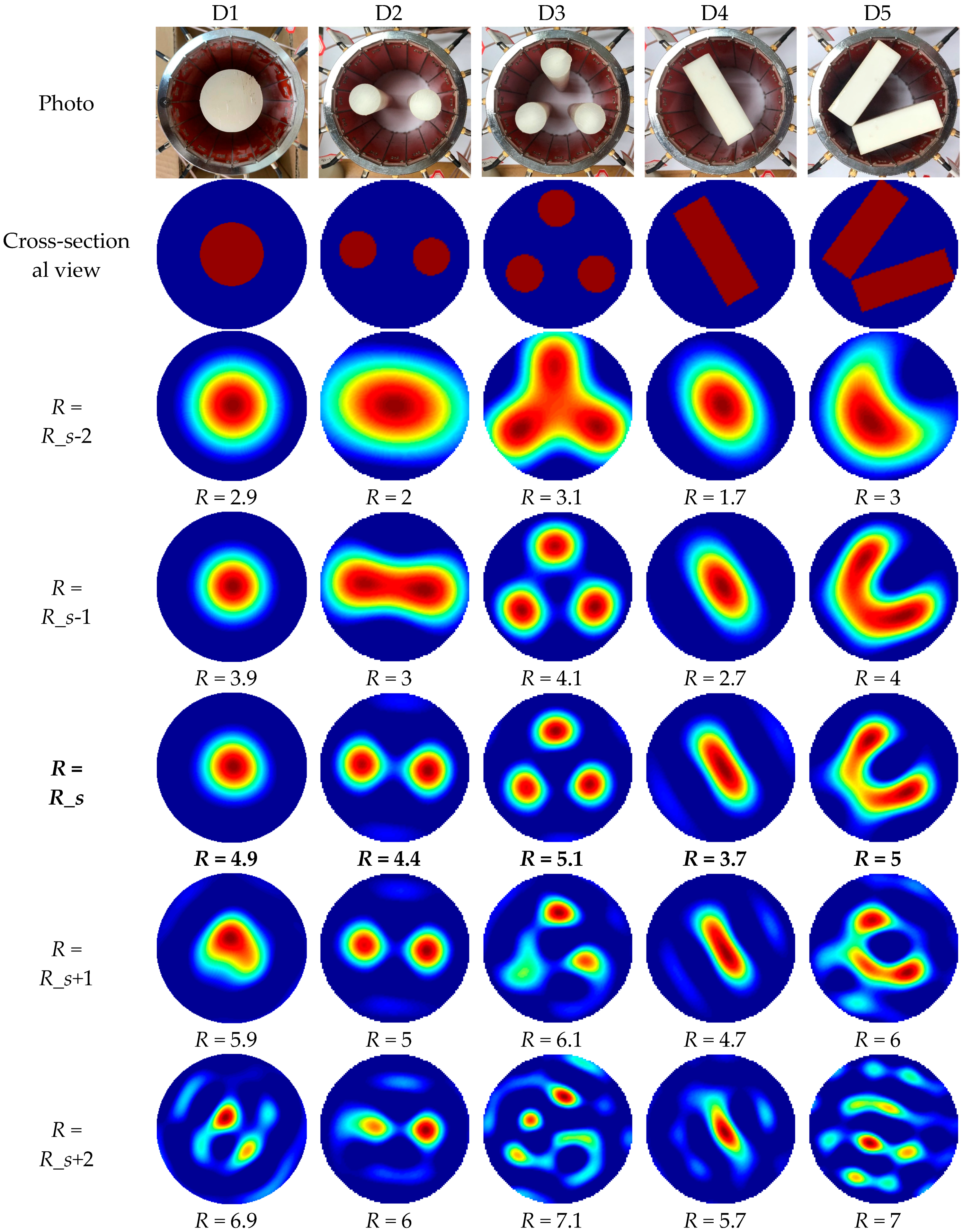
- A small truncation radius means that the reconstructed image contains few high frequency components. The low frequency components contribute to the slowly-changing part in the image. If the truncation radius becomes larger, the images contain more high frequency components and the contours and boundary details of the objects become clearer. However, the noises and artifacts increase;
- (2)
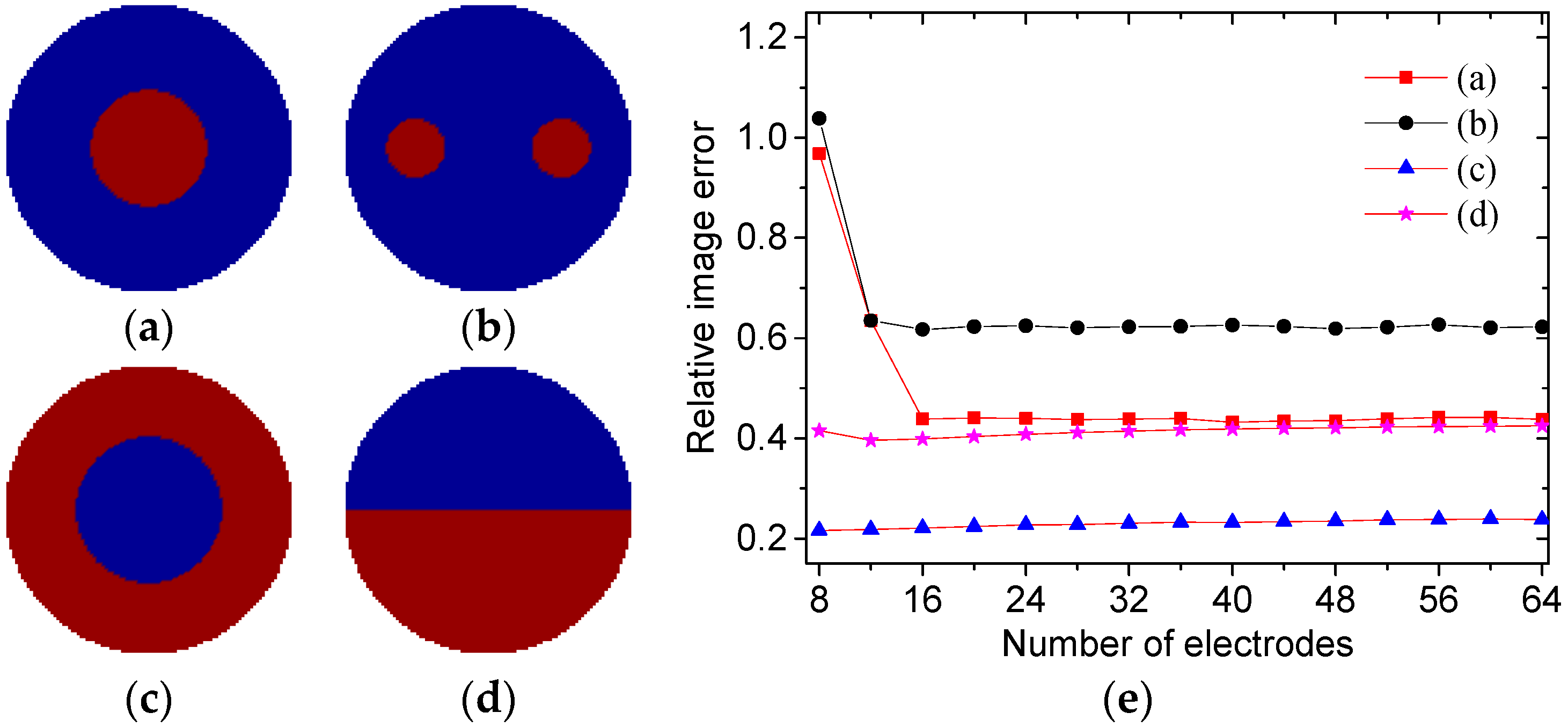
- The permittivity distributions can be divided into two categories, i.e., the core-type and the annular distributions. For the core-type permittivity distributions, i.e., the region of high permittivity is enclosed by a continuous region of low permittivity, the truncation radius should be between 4 and 6 to obtain a better image quality. For annular and stratified distributions, i.e., the region of high permittivity contacts the boundary of the sensing region, the suitable truncation radius should be between 2 and 4, which is much lower than that for core-type distributions. For a higher noise level, a smaller truncation radius should be selected;
- (3)
- The amplitude and phase information of the scattering transform are combined to determine a suitable truncation radius. The experimental results show that small relative image error and good visual effect can be obtained by using the truncation radius selected by the proposed method.
Author Contributions
Funding
Conflicts of Interest
References
- Yang, W.Q. Hardware design of electrical capacitance tomography systems. Meas. Sci. Technol. 1996, 7, 225–232. [Google Scholar] [CrossRef]
- Meribout, M.; Saied, I.M. Real-Time Two-Dimensional Imaging of Solid Contaminants in Gas Pipelines Using an Electrical Capacitance Tomography System. IEEE Trans. Ind. Electron. 2017, 64, 3989–3996. [Google Scholar] [CrossRef]
- Sun, S.; Zhang, W.; Sun, J.; Cao, Z.; Xu, L.; Yan, Y. Real-Time Imaging and Holdup Measurement of Carbon Dioxide Under CCS Conditions Using Electrical Capacitance Tomography. IEEE Sens. J. 2018, 18, 7551–7559. [Google Scholar] [CrossRef]
- Zainal-Mokhtar, K.; Mohamad-Saleh, J. An Oil Fraction Neural Sensor Developed Using Electrical Capacitance Tomography Sensor Data. Sensors 2013, 13, 11385–11406. [Google Scholar] [CrossRef] [PubMed]
- Chandrasekera, T.C.; Li, Y.; Moody, D.; Schnellmann, M.A.; Dennis, J.S.; Holland, D.J. Measurement of bubble sizes in fluidised beds using electrical capacitance tomography. Chem. Eng. Sci. 2015, 126, 679–687. [Google Scholar] [CrossRef]
- Hu, D.; Cao, Z.; Sun, S.; Sun, J.; Xu, L. Dual-Modality Electrical Tomography for Flame Monitoring. IEEE Sens. J. 2018, 18, 8847–8854. [Google Scholar] [CrossRef]
- Sun, S.; Cao, Z.; Huang, A.; Xu, L.; Yang, W. A High-Speed Digital Electrical Capacitance Tomography System Combining Digital Recursive Demodulation and Parallel Capacitance Measurement. IEEE Sens. J. 2017, 17, 6690–6698. [Google Scholar] [CrossRef]
- Olmos, A.; Primicia, J.; Marron, J. Influence of Shielding Arrangement on ECT Sensors. Sensors 2006, 6, 1118–1127. [Google Scholar] [CrossRef]
- Cui, Z.; Wang, H.; Chen, Z.; Xu, Y.; Yang, W. A high-performance digital system for electrical capacitance tomography. Meas. Sci. Technol. 2011, 22, 055503. [Google Scholar] [CrossRef]
- Xu, L.; Sun, S.; Cao, Z.; Yang, W. Performance analysis of a digital capacitance measuring circuit. Rev. Sci. Instrum. 2015, 86, 054703. [Google Scholar] [CrossRef]
- Wang, F.; Marashdeh, Q.; Fan, L.-S.; Warsito, W. Electrical Capacitance Volume Tomography: Design and Applications. Sensors 2010, 10, 1890–1917. [Google Scholar] [CrossRef]
- Kim, Y.S.; Lee, S.H.; Ijaz, U.Z.; Kim, K.Y.; Choi, B.Y. Sensitivity map generation in electrical capacitance tomography using mixed normalization models. Meas. Sci. Technol. 2007, 18, 2092–2102. [Google Scholar] [CrossRef]
- Yang, W.Q.; Peng, L.H. Image reconstruction algorithms for electrical capacitance tomography. Meas. Sci. Technol. 2003, 14, R1–R13. [Google Scholar] [CrossRef]
- Cui, Z.; Wang, Q.; Xue, Q.; Fan, W.; Zhang, L.; Cao, Z.; Sun, B.; Wang, H.; Yang, W. A review on image reconstruction algorithms for electrical capacitance/resistance tomography. Sens. Rev. 2016, 36, 429–445. [Google Scholar] [CrossRef]
- Tian, W.; Sun, J.; Ramli, M.F.; Yang, W. Adaptive Selection of Relaxation Factor in Landweber Iterative Algorithm. IEEE Sens. J. 2017, 17, 7029–7042. [Google Scholar] [CrossRef]
- Lei, J.; Liu, S.; Wang, X.; Liu, Q. An Image Reconstruction Algorithm for Electrical Capacitance Tomography Based on Robust Principle Component Analysis. Sensors 2013, 13, 2076–2092. [Google Scholar] [CrossRef]
- Cao, Z.; Ji, L.; Xu, L. Iterative Reconstruction Algorithm for Electrical Capacitance Tomography Based on Calderon’s Method. IEEE Sens. J. 2018, 18, 8450–8462. [Google Scholar] [CrossRef]
- Calderón, A.P. On an inverse boundary value problem. Comput. Appl. Math. 2006, 25, 133–138. [Google Scholar] [CrossRef]
- Cao, Z.; Xu, L.; Wang, H. Image reconstruction technique of electrical capacitance tomography for low-contrast dielectrics using Calderon’s method. Meas. Sci. Technol. 2009, 20, 104027. [Google Scholar] [CrossRef]
- Cao, Z.; Xu, L.; Fan, W.; Wang, H. Electrical Capacitance Tomography for Sensors of Square Cross Sections Using Calderon’s Method. IEEE Trans. Instrum. Meas. 2011, 60, 900–907. [Google Scholar] [CrossRef]
- Sun, S.; Xu, L.; Cao, Z.; Sun, J. Influence of the Integral Parameters in Calderon Method on Image Quality for Electrical Capacitance Tomography. Available online: https://www.isipt.org/world-congress/9/29273.html (accessed on 27 March 2019).
- Liang, S.; Ye, J.; Wang, H.; Wu, M.; Yang, W. Influence of the internal wall thickness of electrical capacitance tomography sensors on image quality. Meas. Sci. Technol. 2018, 29, 035401. [Google Scholar] [CrossRef]
- Siltanen, S.; Mueller, J.; Isaacson, D. An implementation of the reconstruction algorithm of A Nachman for the 2D inverse conductivity problem. Inverse Probl. 2000, 16, 681. [Google Scholar] [CrossRef]
- Knudsen, K.; Lassas, M.; Mueller, J.; Siltanen, S. Regularized D-bar method for the inverse conductivity problem. Inverse Probl. Imaging 2009, 3, 599–624. [Google Scholar] [CrossRef]


| R Selected by the Proposed Method | Relative Error Using the Selected R | R with Minimum Relative Error | Minimum Relative Error | ||
|---|---|---|---|---|---|
| Core | without noise | 5 | 50% | 6.6 | 42% |
| 0.01% noise | 4.9 | 52% | 3.1 | 45% | |
| 0.1% noise | 4.7 | 59% | 2.8 | 45% | |
| Multiple objects | without noise | 4.1 | 75% | 5.3 | 61% |
| 0.01% noise | 4.1 | 80% | 5.2 | 62% | |
| 0.1% noise | 3.8 | 96% | 4.3 | 78% | |
| Annular | without noise | 2.4 | 23% | 2.8 | 21% |
| 0.01% noise | 2.4 | 23% | 2.8 | 21% | |
| 0.1% noise | 2.2 | 30% | 2.7 | 22% | |
| Stratified | without noise | 2.4 | 39% | 1.9 | 38% |
| 0.01% noise | 2.4 | 39% | 1.9 | 38% | |
| 0.1% noise | 2.4 | 39% | 1.9 | 38% |
| R Selected by the Proposed Method | Relative Errors Using the Selected R | R with Minimum Relative Errors | Minimum Relative Errors | |
|---|---|---|---|---|
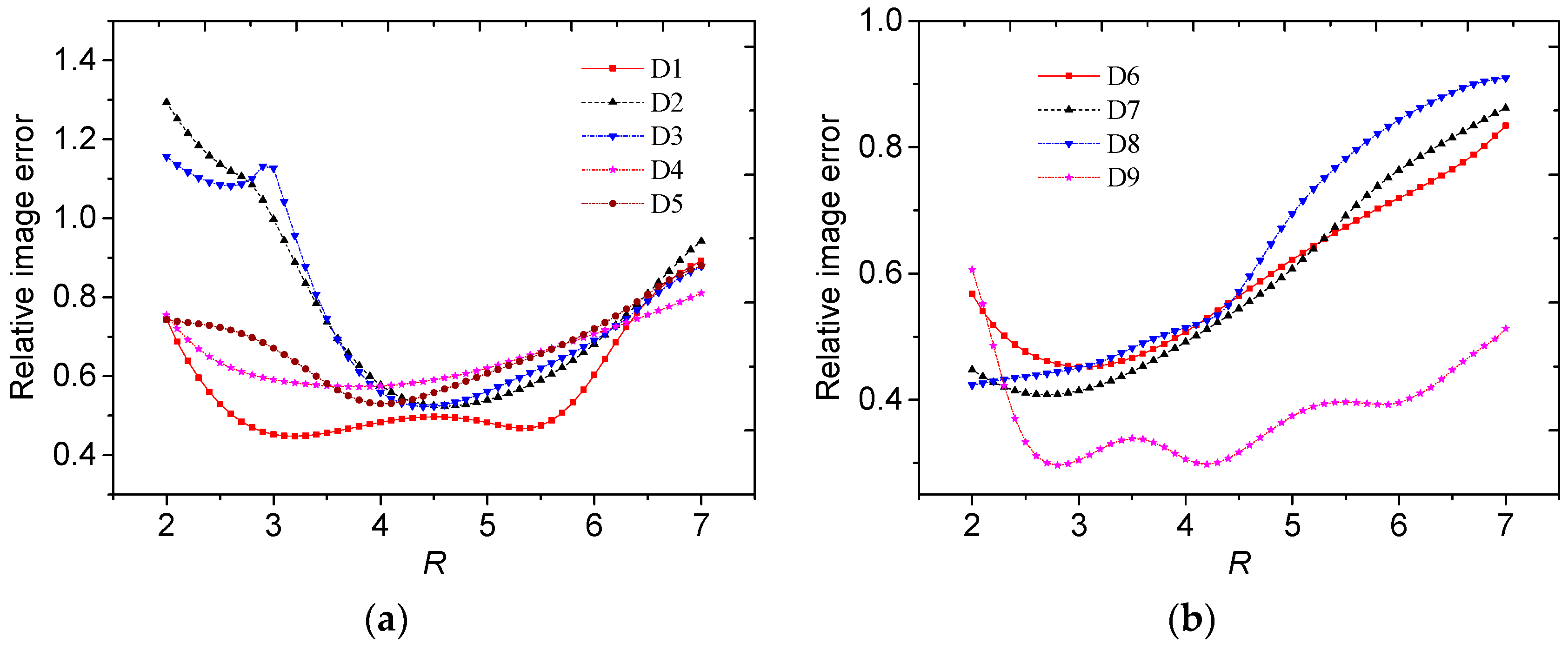
| D1 | 4.9 | 48% | 3.2 | 45% |
| D2 | 4.4 | 53% | 4.6 | 52% |
| D3 | 5.1 | 57% | 4.4 | 52% |
| D4 | 3.7 | 57% | 3.8 | 57% |
| D5 | 5 | 60% | 4 | 52% |
| D6 | 2.6 | 46% | 3 | 45% |
| D7 | 2.6 | 41% | 2.7 | 41% |
| D8 | 2.7 | 44% | 2 | 42% |
| D9 | 3.2 | 32% | 2.8 | 30% |
© 2019 by the authors. Licensee MDPI, Basel, Switzerland. This article is an open access article distributed under the terms and conditions of the Creative Commons Attribution (CC BY) license (http://creativecommons.org/licenses/by/4.0/).
Share and Cite
Sun, S.; Xu, L.; Cao, Z.; Sun, J.; Tian, W. Adaptive Selection of Truncation Radius in Calderon’s Method for Direct Image Reconstruction in Electrical Capacitance Tomography. Sensors 2019, 19, 2014. https://doi.org/10.3390/s19092014
Sun S, Xu L, Cao Z, Sun J, Tian W. Adaptive Selection of Truncation Radius in Calderon’s Method for Direct Image Reconstruction in Electrical Capacitance Tomography. Sensors. 2019; 19(9):2014. https://doi.org/10.3390/s19092014
Chicago/Turabian StyleSun, Shijie, Lijun Xu, Zhang Cao, Jiangtao Sun, and Wenbin Tian. 2019. "Adaptive Selection of Truncation Radius in Calderon’s Method for Direct Image Reconstruction in Electrical Capacitance Tomography" Sensors 19, no. 9: 2014. https://doi.org/10.3390/s19092014
APA StyleSun, S., Xu, L., Cao, Z., Sun, J., & Tian, W. (2019). Adaptive Selection of Truncation Radius in Calderon’s Method for Direct Image Reconstruction in Electrical Capacitance Tomography. Sensors, 19(9), 2014. https://doi.org/10.3390/s19092014