Dynamic Flying Ant Colony Optimization (DFACO) for Solving the Traveling Salesman Problem


Abstract
:1. Introduction
2. Related Work
2.1. Metaheuristic Solutions
2.2. Opt Algorithm
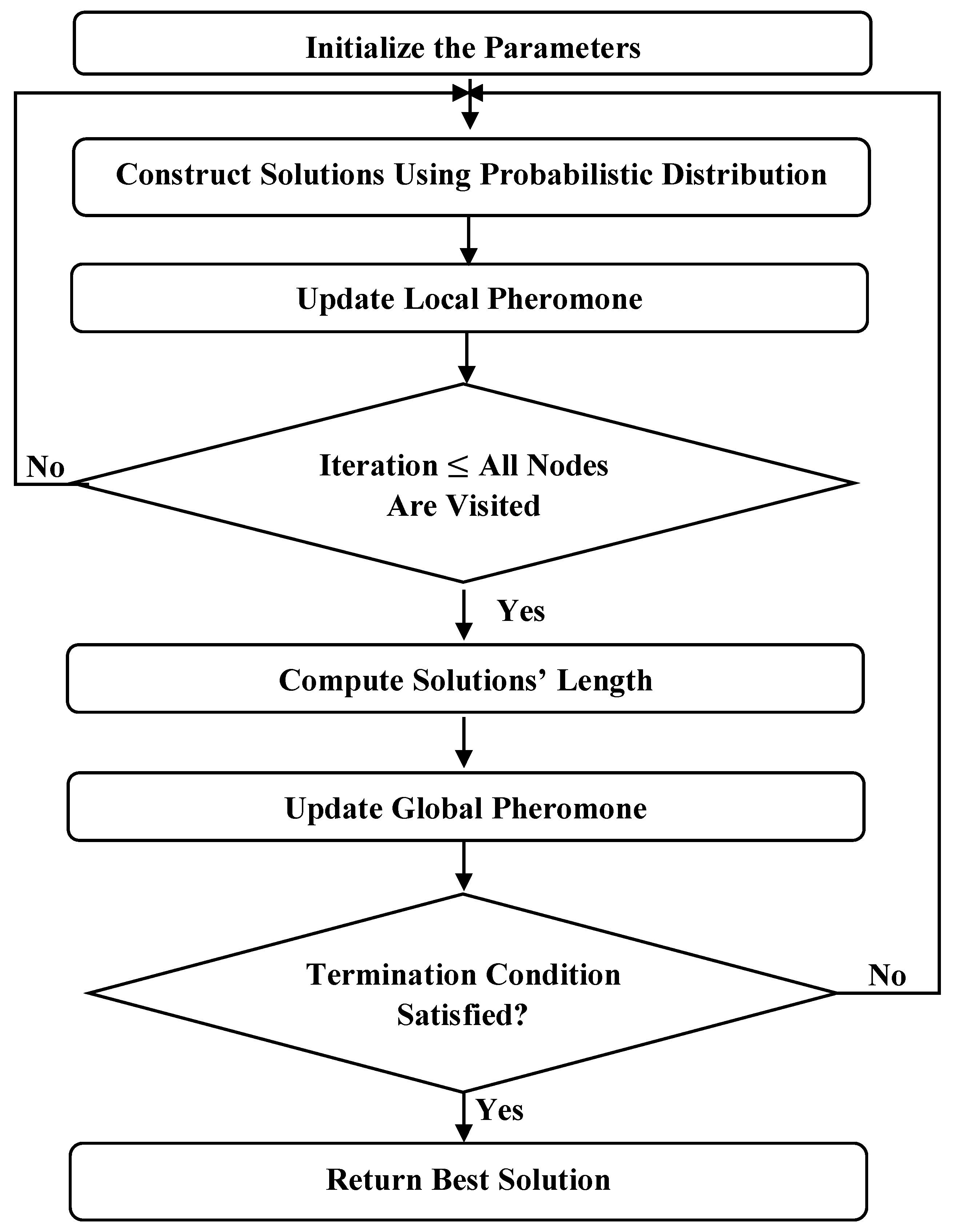
2.3. Ant Colony Optimization
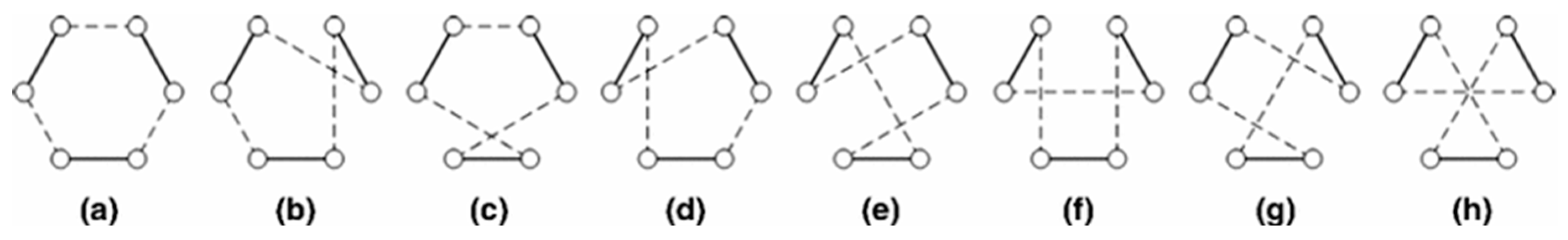
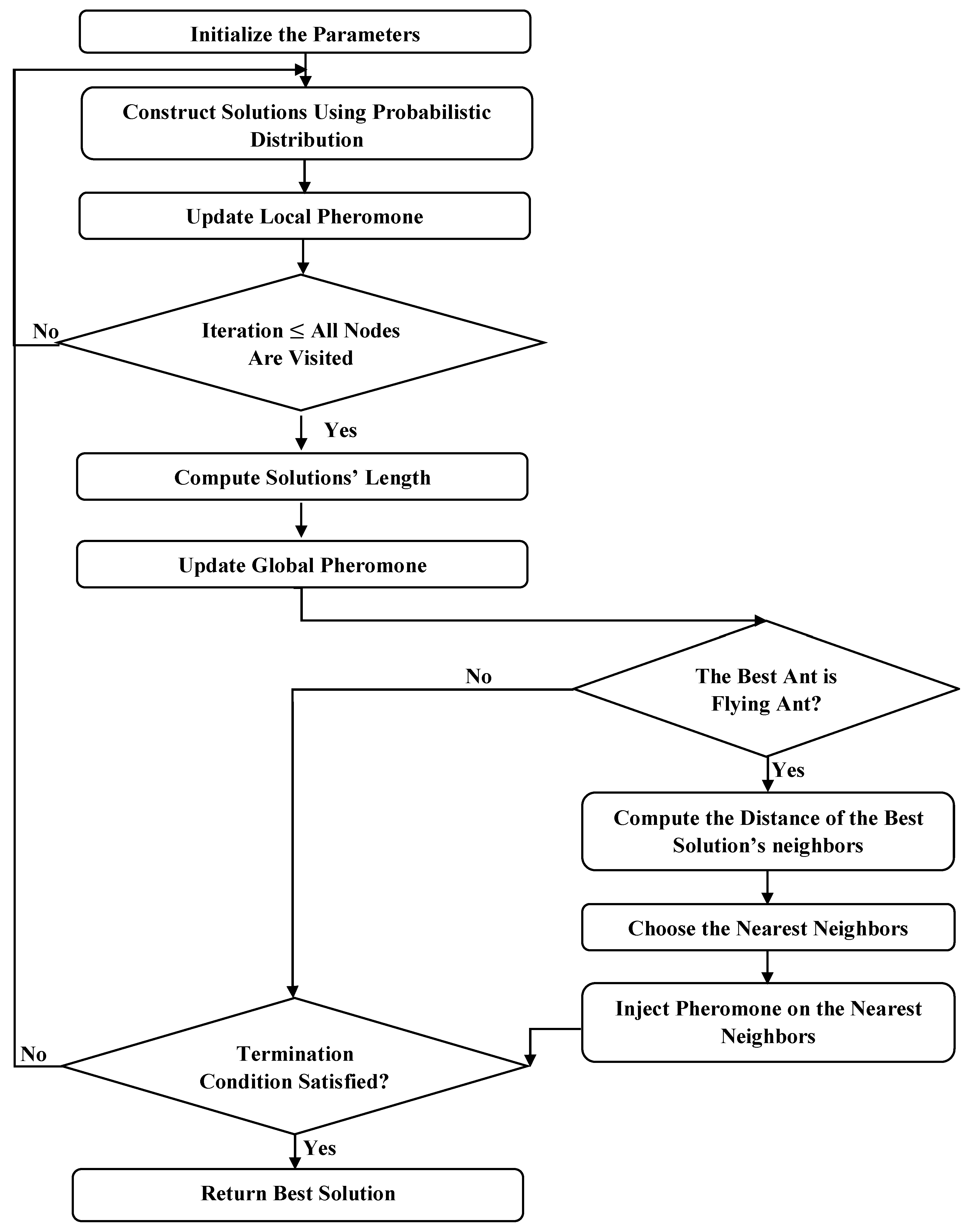
2.4. Flying Ant Colony Optimization
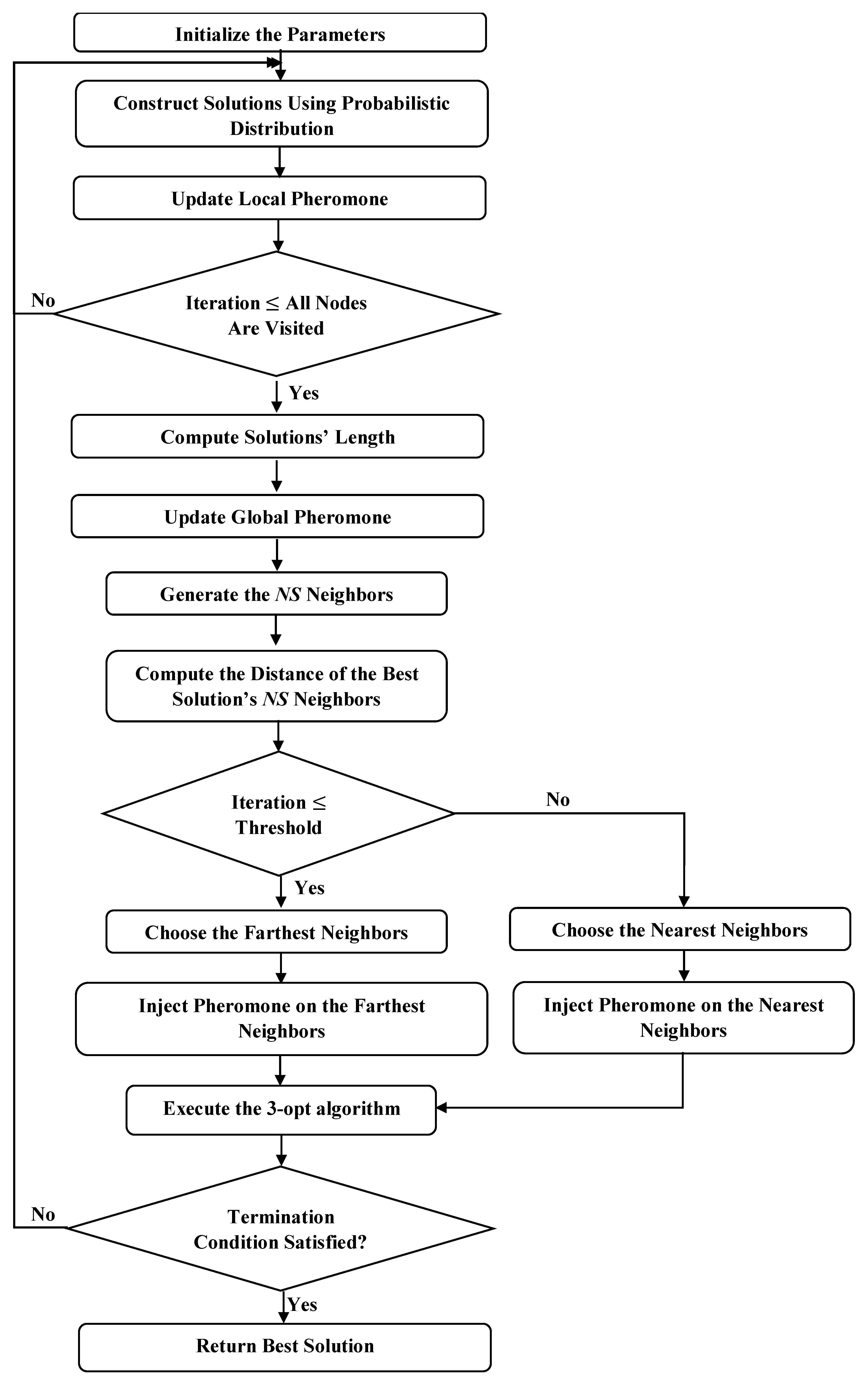
3. Dynamic Flying Ant Colony Optimization (DFACO) Algorithm
4. Experimental Results
5. Conclusions
Author Contributions
Funding
Acknowledgments
Conflicts of Interest
References
- Lenstra, J.K.; Kan, A.R.; Lawler, E.L.; Shmoys, D. The Traveling Salesman Problem: A Guided Tour of Combinatorial Optimization; John Wiley & Sons: Hoboken, NJ, USA, 1985. [Google Scholar]
- Papadimitriou, C.H. The Euclidean travelling salesman problem is NP-complete. Theor. Comput. Sci. 1977, 4, 237–244. [Google Scholar] [CrossRef]
- Garey, M.R.; Graham, R.L.; Johnson, D.S. Some NP-complete geometric problems. In Proceedings of the 8th Annual ACM Symposium on Theory of Computing, Hershey, PA, USA, 3–5 May 1976; pp. 10–22. [Google Scholar]
- Tito, J.E.; Yacelga, M.E.; Paredes, M.C.; Utreras, A.J.; Wójcik, W.; Ussatova, O. Solution of travelling salesman problem applied to Wireless Sensor Networks (WSN) through the MST and B&B methods. In Proceedings of the Photonics Applications in Astronomy, Communications, Industry, and High-Energy Physics Experiments, Wilga, Poland, 3–10 June 2018; p. 108082F. [Google Scholar]
- Kravchuk, S.; Minochkin, D.; Omiotek, Z.; Bainazarov, U.; Weryńska-Bieniasz, R.; Iskakova, A. Cloud-based mobility management in heterogeneous wireless networks. In Proceedings of the Photonics Applications in Astronomy, Communications, Industry, and High Energy Physics Experiments, Wilga, Poland, 28 May–6 June 2017; p. 104451W. [Google Scholar]
- Farrugia, L.I. Wireless Sensor Networks; Nova Science Publishers, Inc.: New York, NY, USA, 2011. [Google Scholar]
- Gülcü, Ş.; Mahi, M.; Baykan, Ö.K.; Kodaz, H. A parallel cooperative hybrid method based on ant colony optimization and 3-Opt algorithm for solving traveling salesman problem. Soft Comput. 2018, 22, 1669–1685. [Google Scholar] [CrossRef]
- Chen, S.-M.; Chien, C.-Y. Solving the traveling salesman problem based on the genetic simulated annealing ant colony system with particle swarm optimization techniques. Expert Syst. Appl. 2011, 38, 14439–14450. [Google Scholar] [CrossRef]
- Deng, W.; Zhao, H.; Zou, L.; Li, G.; Yang, X.; Wu, D. A novel collaborative optimization algorithm in solving complex optimization problems. Soft Comput. 2017, 21, 4387–4398. [Google Scholar] [CrossRef]
- Eskandari, L.; Jafarian, A.; Rahimloo, P.; Baleanu, D. A Modified and Enhanced Ant Colony Optimization Algorithm for Traveling Salesman Problem. In Mathematical Methods in Engineering; Springer: Berlin/Heidelberg, Germany, 2019; pp. 257–265. [Google Scholar]
- Hasan, L.S. Solving Traveling Salesman Problem Using Cuckoo Search and Ant Colony Algorithms. J. Al-Qadisiyah Comput. Sci. Math. 2018, 10, 59–64. [Google Scholar]
- Mavrovouniotis, M.; Müller, F.M.; Yang, S. Ant colony optimization with local search for dynamic traveling salesman problems. IEEE Trans. Cybern. 2017, 47, 1743–1756. [Google Scholar] [CrossRef]
- de S Alves, D.R.; Neto, M.T.R.S.; Ferreira, F.d.S.; Teixeira, O.N. SIACO: A novel algorithm based on ant colony optimization and game theory for travelling salesman problem. In Proceedings of the 2nd International Conference on Machine Learning and Soft Computing, Phu Quoc Island, Viet Nam, 2–4 February 2018; pp. 62–66. [Google Scholar]
- Han, X.-C.; Ke, H.-W.; Gong, Y.-J.; Lin, Y.; Liu, W.-L.; Zhang, J. Multimodal optimization of traveling salesman problem: A niching ant colony system. In Proceedings of the Genetic and Evolutionary Computation Conference Companion, Kyoto, Japan, 15–19 July 2018; pp. 87–88. [Google Scholar]
- Pintea, C.-M.; Pop, P.C.; Chira, C. The generalized traveling salesman problem solved with ant algorithms. Complex Adapt. Syst. Model. 2017, 5, 8. [Google Scholar] [CrossRef]
- Xiao, Y.; Jiao, J.; Pei, J.; Zhou, K.; Yang, X. A Multi-strategy Improved Ant Colony Algorithm for Solving Traveling Salesman Problem. In Proceedings of the IOP Conference Series: Materials Science and Engineering, Shanxi, China, 18–20 May 2018; p. 042101. [Google Scholar]
- Zhou, Y.; He, F.; Qiu, Y. Dynamic strategy based parallel ant colony optimization on GPUs for TSPs. Sci. China Inf. Sci. 2017, 60, 068102. [Google Scholar] [CrossRef]
- Mahi, M.; Baykan, Ö.K.; Kodaz, H. A new hybrid method based on particle swarm optimization, ant colony optimization and 3-opt algorithms for traveling salesman problem. Appl. Soft Comput. 2015, 30, 484–490. [Google Scholar] [CrossRef]
- Khan, I.; Maiti, M.K. A swap sequence based Artificial Bee Colony algorithm for Traveling Salesman Problem. Swarm Evol. Comput. 2019, 44, 428–438. [Google Scholar] [CrossRef]
- Ouaarab, A.; Ahiod, B.; Yang, X.-S. Discrete cuckoo search algorithm for the travelling salesman problem. Neural Comput. Appl. 2014, 24, 1659–1669. [Google Scholar] [CrossRef]
- Osaba, E.; Yang, X.-S.; Diaz, F.; Lopez-Garcia, P.; Carballedo, R. An improved discrete bat algorithm for symmetric and asymmetric Traveling Salesman Problems. Eng. Appl. Artif. Intell. 2016, 48, 59–71. [Google Scholar] [CrossRef]
- Choong, S.S.; Wong, L.-P.; Lim, C.P. An artificial bee colony algorithm with a modified choice function for the Traveling Salesman Problem. Swarm Evol. Comput. 2019, 44, 622–635. [Google Scholar] [CrossRef]
- Civicioglu, P.; Besdok, E. A conceptual comparison of the Cuckoo-search, particle swarm optimization, differential evolution and artificial bee colony algorithms. Artif. Intell. Rev. 2013, 39, 315–346. [Google Scholar] [CrossRef]
- Lin, S. Computer solutions of the traveling salesman problem. Bell Syst. Tech. J. 1965, 44, 2245–2269. [Google Scholar] [CrossRef]
- Dorigo, M.; Stützle, T. Ant colony optimization: Overview and recent advances. In Handbook of Metaheuristics; Springer: Berlin/Heidelberg, Germany, 2019; pp. 311–351. [Google Scholar]
- Reinelt, G. The Traveling Salesman: Computational Solutions for TSP Applications; Springer: Berlin/Heidelberg, Germany, 1994. [Google Scholar]
- Blazinskas, A.; Misevicius, A. combining 2-opt, 3-opt and 4-opt with k-swap-kick perturbations for the traveling salesman problem. In Proceedings of the 17th International Conference on Information and Software Technologies, Kaunas, Lithuania, 27–29 April 2011; pp. 50–401. [Google Scholar]
- Dorigo, M.; Gambardella, L.M. Ant colony system: A cooperative learning approach to the traveling salesman problem. IEEE Trans. Evol. Comput. 1997, 1, 53–66. [Google Scholar] [CrossRef]
- Dorigo, M.; Gambardella, L.M. Ant colonies for the travelling salesman problem. BioSystems 1997, 43, 73–81. [Google Scholar] [CrossRef]
- Gambardella, L.M.; Dorigo, M. Solving Symmetric and Asymmetric TSPs by Ant Colonies. In Proceedings of the International Conference on Evolutionary Computation, Nagoya, Japan, 20–22 May 1996; pp. 622–627. [Google Scholar]
- Deepa, O.; Senthilkumar, A. Swarm intelligence from natural to artificial systems: Ant colony optimization. Networks (Graph-Hoc) 2016, 8, 9–17. [Google Scholar]
- Aljanaby, A. An Experimental Study of the Search Stagnation in Ants Algorithms. Int. J. Comput. Appl. 2016, 148. [Google Scholar] [CrossRef]
- Dahan, F.; El Hindi, K.; Ghoneim, A. An Adapted Ant-Inspired Algorithm for Enhancing Web Service Composition. Int. J. Semant. Web Inf. Syst. 2017, 13, 181–197. [Google Scholar] [CrossRef]
- Reinelt, G. TSPLIB—A traveling salesman problem library. Orsa J. Comput. 1991, 3, 376–384. [Google Scholar] [CrossRef]


| Parameters | Value |
|---|---|
| α | 1 |
| β | 2 |
| ρ | 0.1 |
| τ0 | 0.1 |
| S | 100 |
| Z | 100 |
| Th (for DFACO) | 80 |
| TSP Instance | BKS | ACO with 3-Opt | The Proposed Method | ||||||
|---|---|---|---|---|---|---|---|---|---|
| Mean | SD | Best | Time | Mean | SD | Best | Time | ||
| eil51 | 426 | 426.00 | 0.00 | 426.00 | 1 | 426.00 | 0.00 | 426.00 | 1 |
| eil76 | 538 | 538.00 | 0.00 | 538.00 | 3 | 538.00 | 0.00 | 538.00 | 3 |
| eil101 | 629 | 629.00 | 0.00 | 629.00 | 10 | 629.00 | 0.00 | 629.00 | 12 |
| berlin52 | 7542 | 7542.00 | 0.00 | 7542.00 | 1 | 7542.00 | 0.00 | 7542.00 | 1 |
| bier127 | 118,282 | 118,282.00 | 0.00 | 118,282.00 | 56 | 118,282.00 | 0.00 | 118,282.00 | 47 |
| ch130 | 6110 | 6110.00 | 0.00 | 6110.00 | 16 | 6110.00 | 0.00 | 6110.00 | 13 |
| ch150 | 6528 | 6528.00 | 0.00 | 6528.00 | 17 | 6528.00 | 0.00 | 6528.00 | 24 |
| rd100 | 7910 | 7910.00 | 0.00 | 7910.00 | 2 | 7910.00 | 0.00 | 7910.00 | 2 |
| lin105 | 14,379 | 14,379.00 | 0.00 | 14,379.00 | 2 | 14,379.00 | 0.00 | 14,379.00 | 2 |
| lin318 | 42,029 | 42,243.70 | 52.27 | 42,135.00 | 349 | 42,228.03 | 48.30 | 42,123.00 | 381 |
| kroA100 | 21,282 | 21,282.00 | 0.00 | 21,282.00 | 2 | 21,282.00 | 0.00 | 21,282.00 | 2 |
| kroA150 | 26,524 | 26,524.07 | 0.25 | 26,524.00 | 83 | 26,524.03 | 0.18 | 26,524.00 | 57 |
| kroA200 | 29,368 | 29,378.73 | 11.09 | 29,368.00 | 211 | 29,368.00 | 0.00 | 29,368.00 | 168 |
| kroB100 | 22,141 | 22,141.00 | 0.00 | 22,141.00 | 2 | 22,141.00 | 0.00 | 22,141.00 | 2 |
| kroB150 | 26,130 | 26,130.00 | 0.00 | 26,130.00 | 9 | 26,130.00 | 0.00 | 26,130.00 | 7 |
| kroB200 | 29,437 | 29,443.20 | 7.07 | 29,437.00 | 137 | 29,441.60 | 5.16 | 29,437.00 | 185 |
| kroC100 | 20,749 | 20,749.00 | 0.00 | 20,749.00 | 2 | 20,749.00 | 0.00 | 20,749.00 | 2 |
| kroD100 | 21,294 | 21,294.00 | 0.00 | 21,294.00 | 3 | 21,294.00 | 0.00 | 21,294.00 | 3 |
| kroE100 | 22,068 | 22,068.00 | 0.00 | 22,068.00 | 2 | 22,068.00 | 0.00 | 22,068.00 | 2 |
| rat575 | 6773 | 6384.87 | 7.21 | 6368.00 | 443 | 6367.3 | 8.48 | 6348.00 | 126.2 |
| rat783 | 8806 | 10,524.60 | 13.36 | 10,483.00 | 922 | 10,491.9 | 14.62 | 10,455.00 | 151.6 |
| rl1323 | 270,199 | 273,969.57 | 515.57 | 272,639.00 | 2267 | 273,367.9 | 484.78 | 272,487.00 | 2285 |
| fl1400 | 20,127 | 20,291.77 | 29.01 | 20,225.00 | 2471 | 20,300.77 | 35.27 | 20,239.00 | 2452 |
| d1655 | 62,128 | 63,722.20 | 95.53 | 63,520.00 | 1754 | 63,707.87 | 114.84 | 63,428.00 | 1523 |
| TSP Instance | BKS | Best Tour Length | Worst Tour Length | Average Tour Length | Time (s) | ||||
|---|---|---|---|---|---|---|---|---|---|
| DFACO | PACO-3Opt | DFACO | PACO-3Opt | DFACO | PACO-3Opt | DFACO | PACO-3Opt | ||
| Eil51 | 426 | 426 | 426 | 426 | 427 | 426 | 426.35 | 1 | 2.39 |
| Berlin52 | 7542 | 7542 | 7542 | 7542 | 7542 | 7542 | 7542 | 1 | 2.1 |
| Rat99 | 1211 | 1211 | 1213 | 1211 | 1225 | 1211 | 1217.1 | 4 | 19.79 |
| Eil76 | 538 | 538 | 538 | 538 | 542 | 538 | 539.85 | 3 | 8.18 |
| St70 | 675 | 675 | 676 | 675 | 679 | 675 | 677.85 | 5.6 | 6.97 |
| KroA100 | 21,282 | 21,282 | 21,282 | 21,282 | 21,382 | 21,282 | 21,326.8 | 2 | 21.1 |
| Lin105 | 14,379 | 14,379 | 14,379 | 14,379 | 14,422 | 14,379 | 14,393 | 2 | 14.57 |
| KroA200 | 29,368 | 29,368 | 29,533 | 29,368 | 29,721 | 29,368 | 29,644.5 | 168 | 213.12 |
| Ch150 | 6528 | 6528 | 6570 | 6528 | 6627 | 6528 | 6601.4 | 24 | 79.35 |
| Eil101 | 629 | 629 | 629 | 629 | 639 | 629 | 630.55 | 12 | 20.79 |
| TSP Instance | BKS | Best Tour Length | Worst Tour Length | Average Tour Length | Time (s) | ||||
|---|---|---|---|---|---|---|---|---|---|
| DFACO | PACO-3Opt | DFACO | PACO-3Opt | DFACO | PACO-3Opt | DFACO | PACO-3Opt | ||
| rd400 | 15,281.0 | 15,321.0 | 15,578.0 | 15,428.0 | 15,667.0 | 15,384.0 | 15,613.9 | 133.1 | 1496.0 |
| fl417 | 11,861.0 | 11,867.0 | 11,972.0 | 11,900.0 | 12,000.0 | 11,880.3 | 11,987.4 | 95.2 | 2046.0 |
| pr439 | 107,217.0 | 107,310.0 | 108,482.0 | 107,698.0 | 108,973.0 | 107,515.9 | 108,702.0 | 142.6 | 2132.0 |
| pcb442 | 50,778.0 | 50,910.0 | 51,962.0 | 51,186.0 | 52,283.0 | 51,047.4 | 52,202.4 | 129.4 | 2088.0 |
| d493 | 35,002.0 | 35,124 | 35,735.0 | 35,380 | 35,982.0 | 35,266.4 | 35,841.0 | 137.59 | 3175.0 |
| u574 | 36,905.0 | 37,168.0 | 37,981.0 | 37,518.0 | 38,165.0 | 37,366.8 | 38,030.7 | 116.9 | 5460.0 |
| rat575 | 6773.0 | 6348.0 | 7003.0 | 6380.0 | 7037.0 | 6367.3 | 7012.4 | 126.2 | 5004.0 |
| p654 | 34,643.0 | 34,695.0 | 35,045.0 | 34,864.0 | 35,116.0 | 34,740.6 | 35,075.0 | 101.7 | 9105.0 |
| d657 | 48,912.0 | 49,250.0 | 50,206.0 | 49,618.0 | 50,386.0 | 49,462.7 | 50,277.5 | 135.1 | 8715.0 |
| u724 | 41,910.0 | 42,284.0 | 42,764.0 | 42,634.0 | 43,272.0 | 42,437.8 | 43,122.5 | 137.0 | 11,458.0 |
| rat783 | 8806.0 | 10,455.0 | 9111.0 | 10,522.0 | 9152.0 | 10,491.9 | 9127.3 | 151.6 | 14,277.0 |
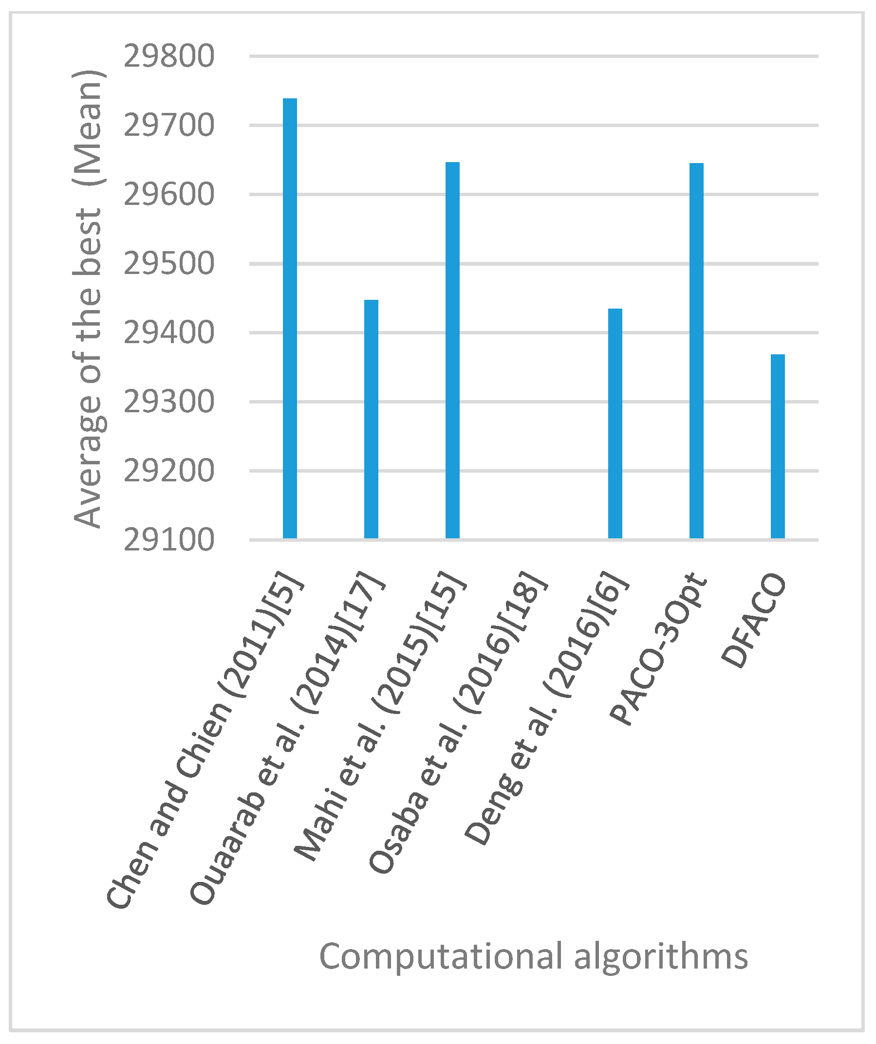
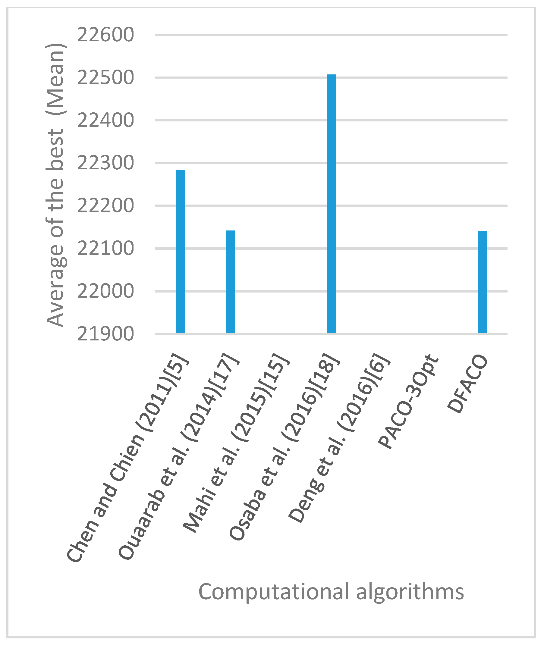
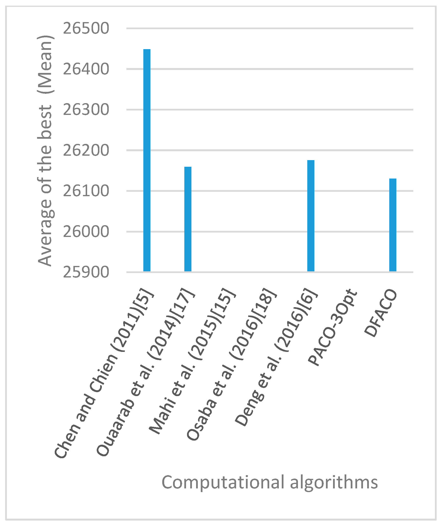
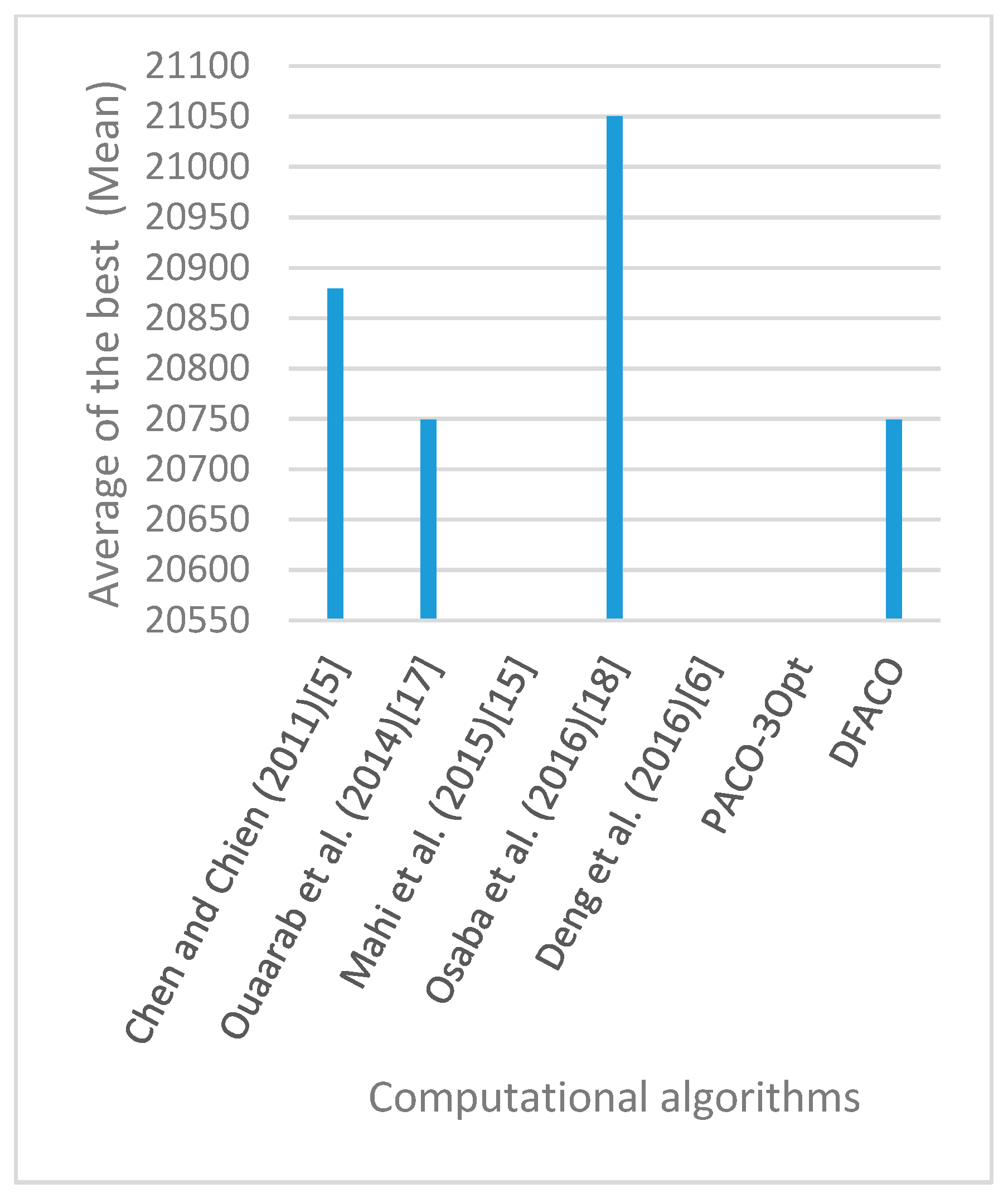
| TSP Instance | BKS | Chen and Chien (2011) [8] | Ouaarab et al. (2014) [20] | Mahi et al. (2015) [18] | Osaba et al. (2016) [21] | Deng et al. (2016) [9] | DFACO | ||||||||||||
|---|---|---|---|---|---|---|---|---|---|---|---|---|---|---|---|---|---|---|---|
| Mean | SD | Best | Mean | SD | Best | Mean | SD | Best | Mean | SD | Best | Mean | SD | Best | Mean | SD | Best | ||
| eil51 | 426 | 427.27 | 0.45 | 427 | 426 | 0 | 426 | 426.45 | 0.61 | 426 | 428.1 | 1.6 | 426 | 427.21 | NA | 426 | 426 | 0 | 426 |
| eil76 | 538 | 540.2 | 2.94 | 538 | 538.03 | 0.17 | 538 | 538.3 | 0.47 | 538 | 548.1 | 3.8 | 539 | 540.302 | NA | 539.153 | 538 | 0 | 538 |
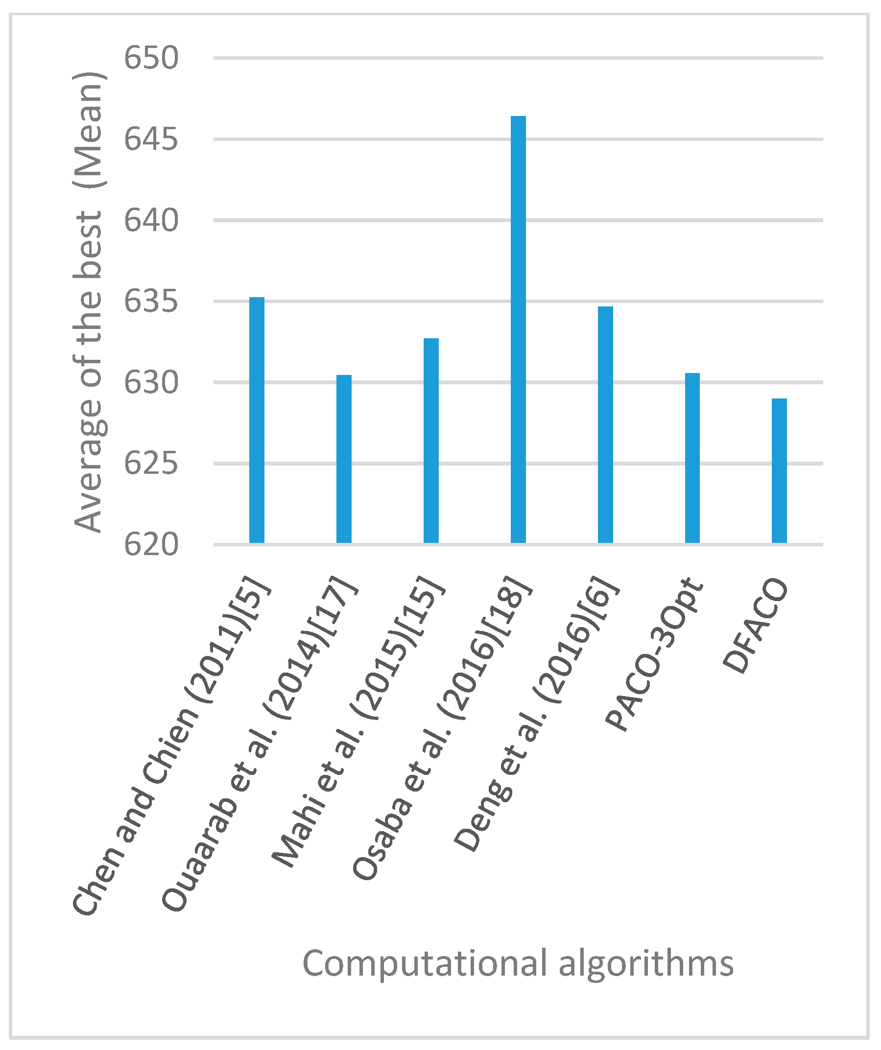
| eil101 | 629 | 635.23 | 3.59 | 630 | 630.43 | 1.14 | 629 | 632.7 | 2.12 | 631 | 646.4 | 4.9 | 634 | 634.68 | NA | 630.01 | 629 | 0 | 629 |
| berlin52 | 7542 | 7542 | 0 | 7542 | 7542 | 0 | 7542 | 7543.2 | 2.37 | 7542 | 7542 | 0 | 7542 | NA | NA | NA | 7542 | 0 | 7542 |
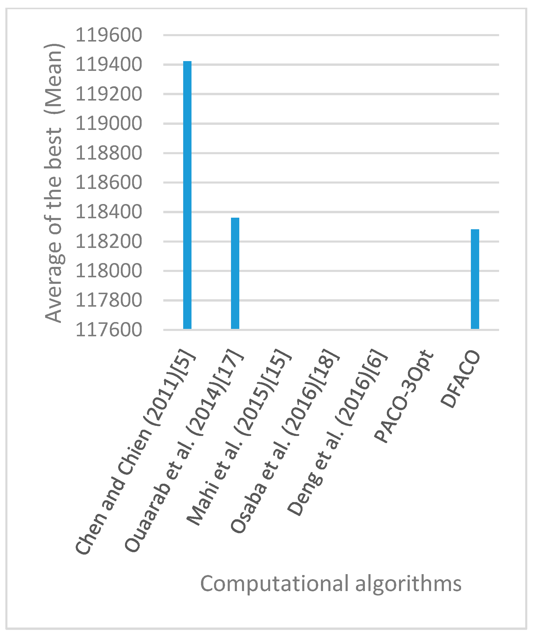
| bier127 | 118,282 | 119,421.8 | 580.83 | 118,282 | 118,360 | 12.73 | 118,282 | NA | NA | NA | NA | NA | NA | NA | NA | NA | 118,282 | 0 | 118,282 |
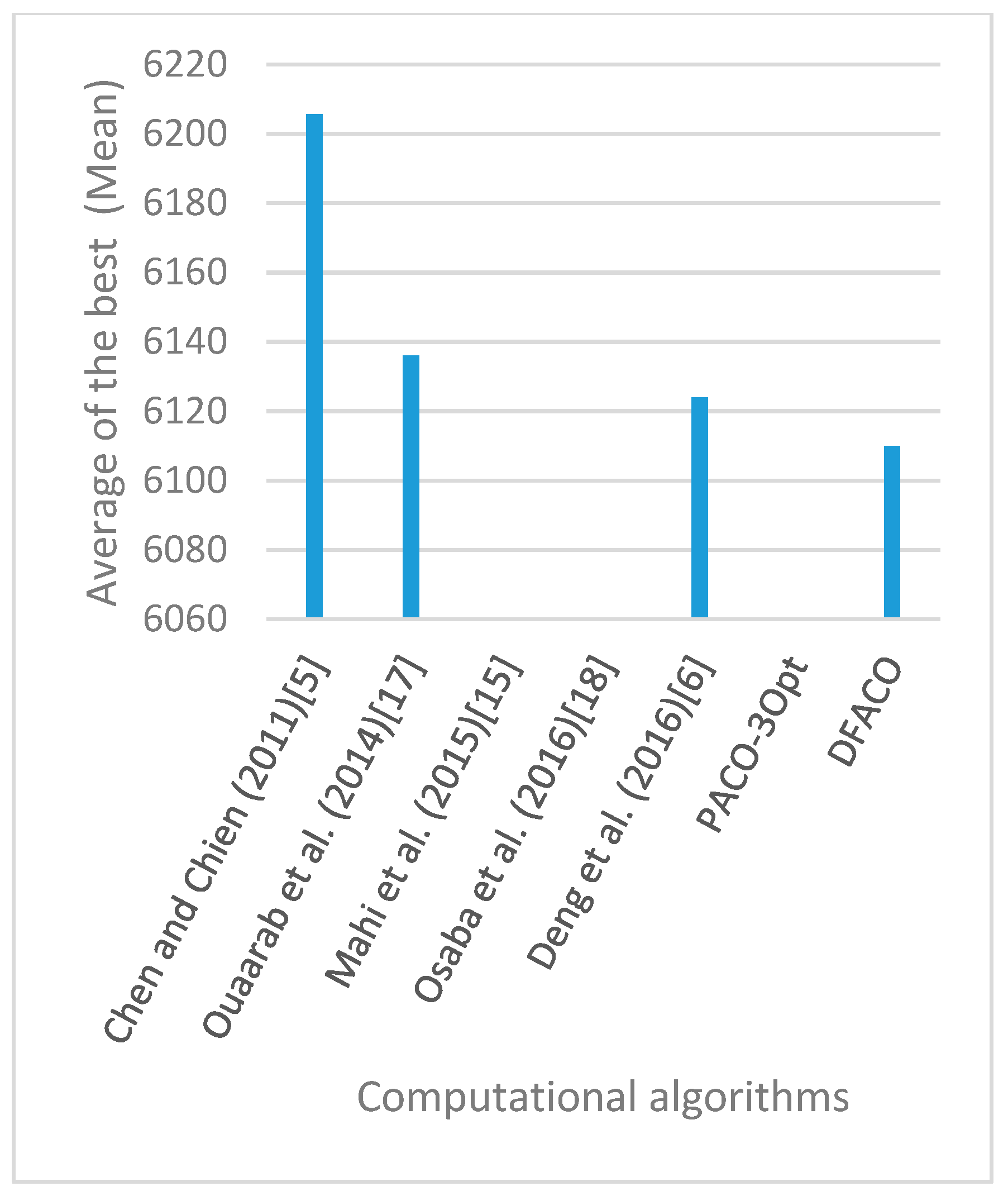
| ch130 | 6110 | 6205.63 | 43.7 | 6141 | 6136 | 21.24 | 6110 | NA | NA | NA | NA | NA | NA | 6123.92 | NA | 6113.26 | 6110 | 0 | 6110 |
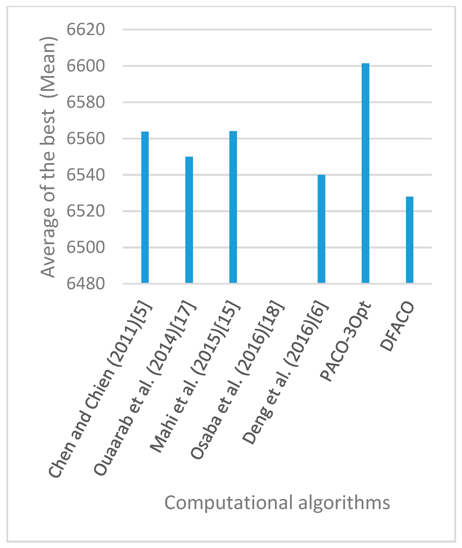
| ch150 | 6528 | 6563.7 | 22.45 | 6528 | 6549.9 | 20.51 | 6528 | 6563.95 | 27.6 | 6538 | NA | NA | NA | 6539.86 | NA | 6528 | 6528 | 0 | 6528 |
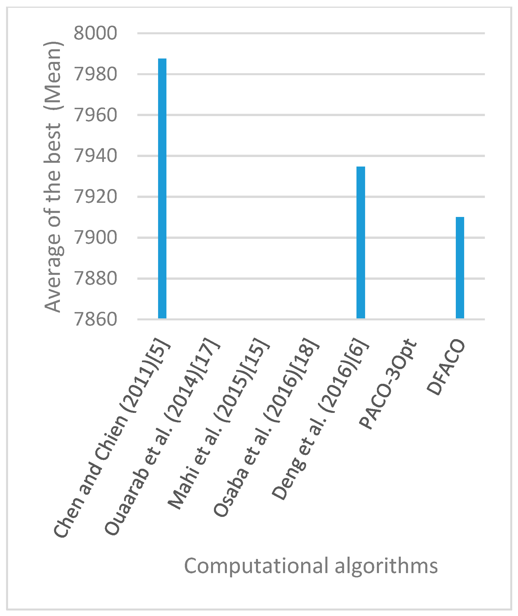
| rd100 | 7910 | 7987.57 | 62.06 | 7910 | NA | NA | NA | NA | NA | NA | NA | NA | NA | 7934.69 | NA | 7910 | 7910 | 0 | 7910 |
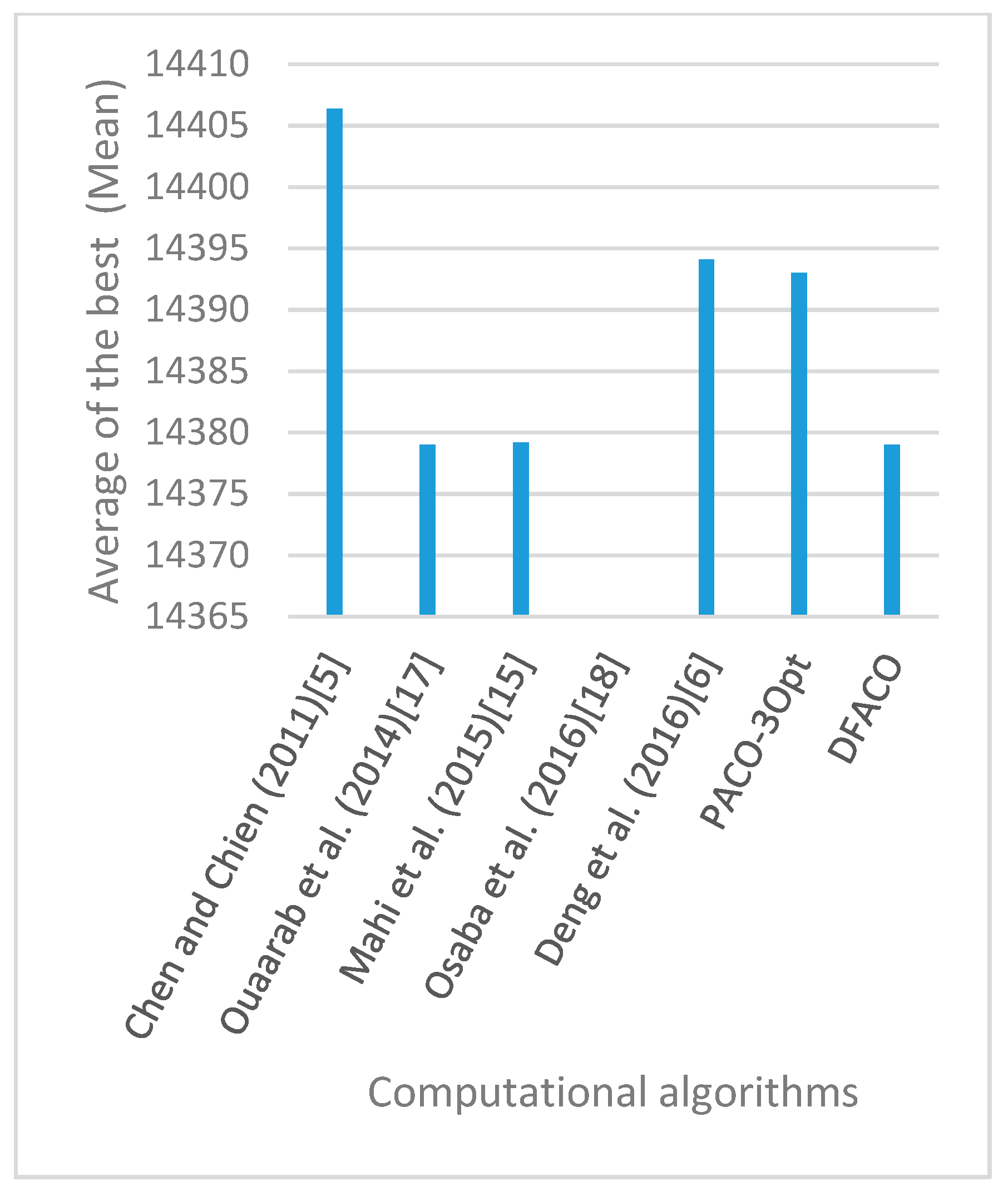
| lin105 | 14,379 | 14,406.37 | 37.28 | 14,379 | 14,379 | 0 | 14,379 | 14,379.2 | 0.48 | 14,379 | NA | NA | NA | 14,394.1 | NA | 14,381.8 | 14,379 | 0 | 14,379 |
| lin318 | 42,029 | 43,002.9 | 307.51 | 42,487 | 42,435 | 185.4 | 42,125 | NA | NA | NA | NA | NA | NA | 42,368.3 | NA | 42,284.9 | 42,228.03 | 48.3 | 42,123 |
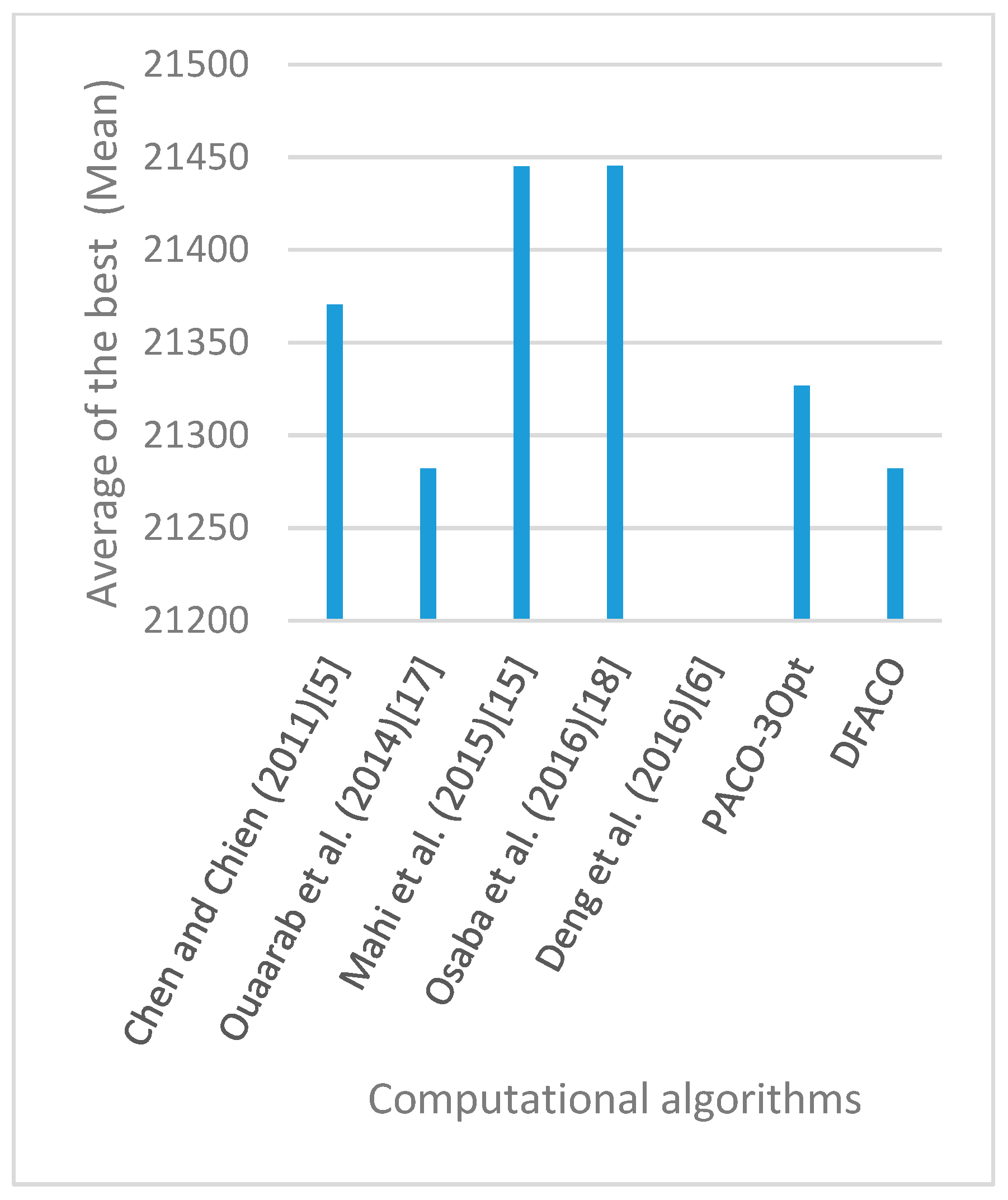
| kroA100 | 21,282 | 21,370.47 | 123.36 | 21,282 | 21,282 | 0 | 21,282 | 21,445.1 | 78.2 | 21,301 | 21,445.3 | 116.5 | 21,282 | NA | NA | NA | 21,282 | 0 | 21,282 |
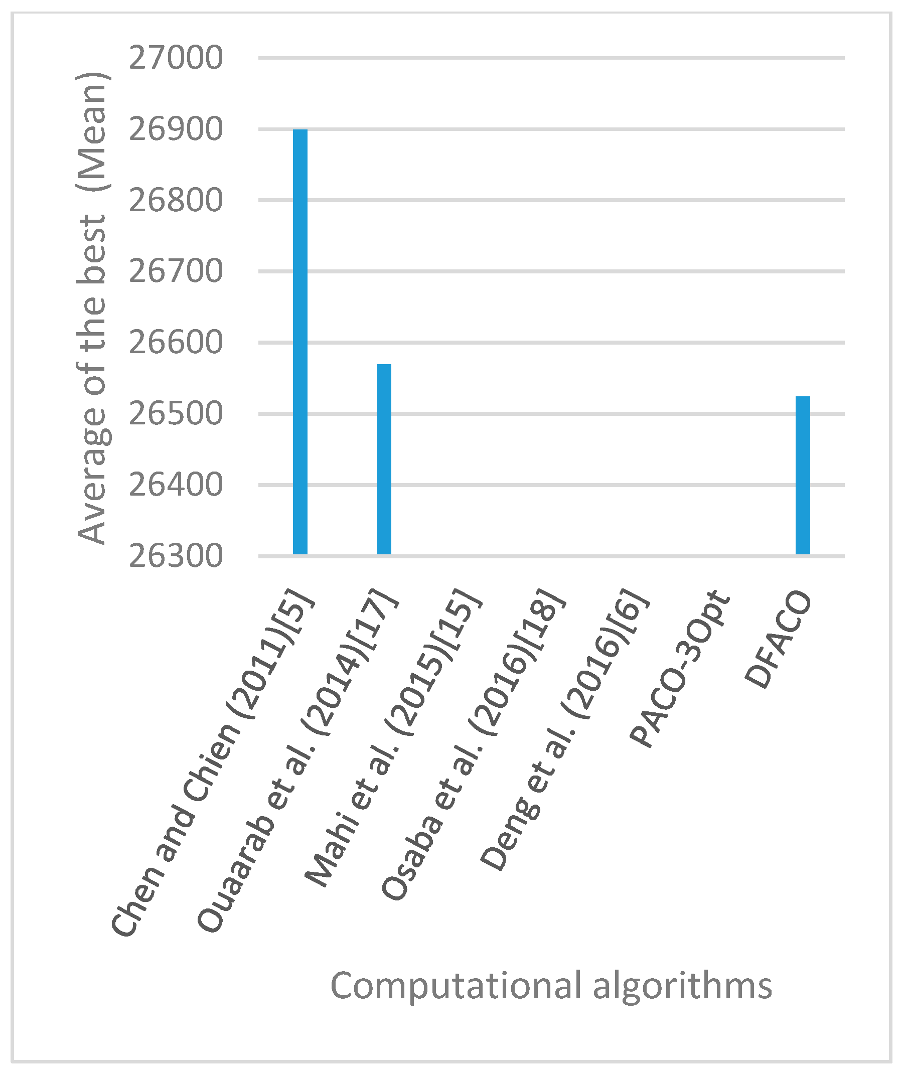
| kroA150 | 26,524 | 26,899.2 | 133.02 | 26,524 | 26,569 | 56.26 | 26,524 | NA | NA | NA | NA | NA | NA | NA | NA | NA | 26,524.03 | 0.18 | 26,524 |
| kroA200 | 29,368 | 29,738.73 | 356.07 | 29,383 | 29,447 | 95.68 | 29,382 | 29,646.1 | 115 | 29,468 | NA | NA | NA | 29,434.7 | NA | 29,380.2 | 29,368 | 0 | 29,368 |
| kroB100 | 22,141 | 22,282.87 | 183.99 | 22,141 | 22,142 | 2.87 | 22,141 | NA | NA | NA | 22,506.4 | 221.3 | 22,140 | NA | NA | NA | 22,141 | 0 | 22,141 |
| kroB150 | 26,130 | 26,448.33 | 266.76 | 26,130 | 26,159 | 34.72 | 26,130 | NA | NA | NA | NA | NA | NA | 26,175.3 | NA | 26,139.4 | 26,130 | 0 | 26,130 |
| kroB200 | 29,437 | 30,035.23 | 357.48 | 29,541 | 29,542 | 92.17 | 29,448 | NA | NA | NA | NA | NA | NA | 29,512.4 | NA | 29,502.6 | 29,441.6 | 5.161 | 29,437 |
| kroC100 | 20,749 | 20,878.97 | 158.64 | 20,749 | 20,749 | 0 | 20,749 | NA | NA | NA | 21,050 | 164.7 | 20,749 | NA | NA | NA | 20,749 | 0 | 20,749 |
| kroD100 | 21,294 | 21,620.47 | 226.6 | 21,309 | 21,304 | 21.79 | 21,294 | NA | NA | NA | 21,593.4 | 141.6 | 21,294 | NA | NA | NA | 21,294 | 0 | 21,294 |
| kroE100 | 22,068 | 22,183.47 | 103.32 | 22,068 | 22,081 | 18.5 | 22,068 | NA | NA | NA | 22,349.6 | 169.6 | 22,068 | NA | NA | NA | 22,068 | 0 | 22,068 |
| rat575 | 6773 | 6933.87 | 27.62 | 6891 | NA | NA | NA | NA | NA | NA | NA | NA | NA | 6901.25 | NA | 6859.85 | 6367.3 | 8.48 | 6348 |
| rat783 | 8806 | 9079.23 | 52.69 | 8988 | NA | NA | NA | NA | NA | NA | NA | NA | NA | 8976.92 | NA | 8940.37 | 10,491.9 | 14.62 | 10,455 |
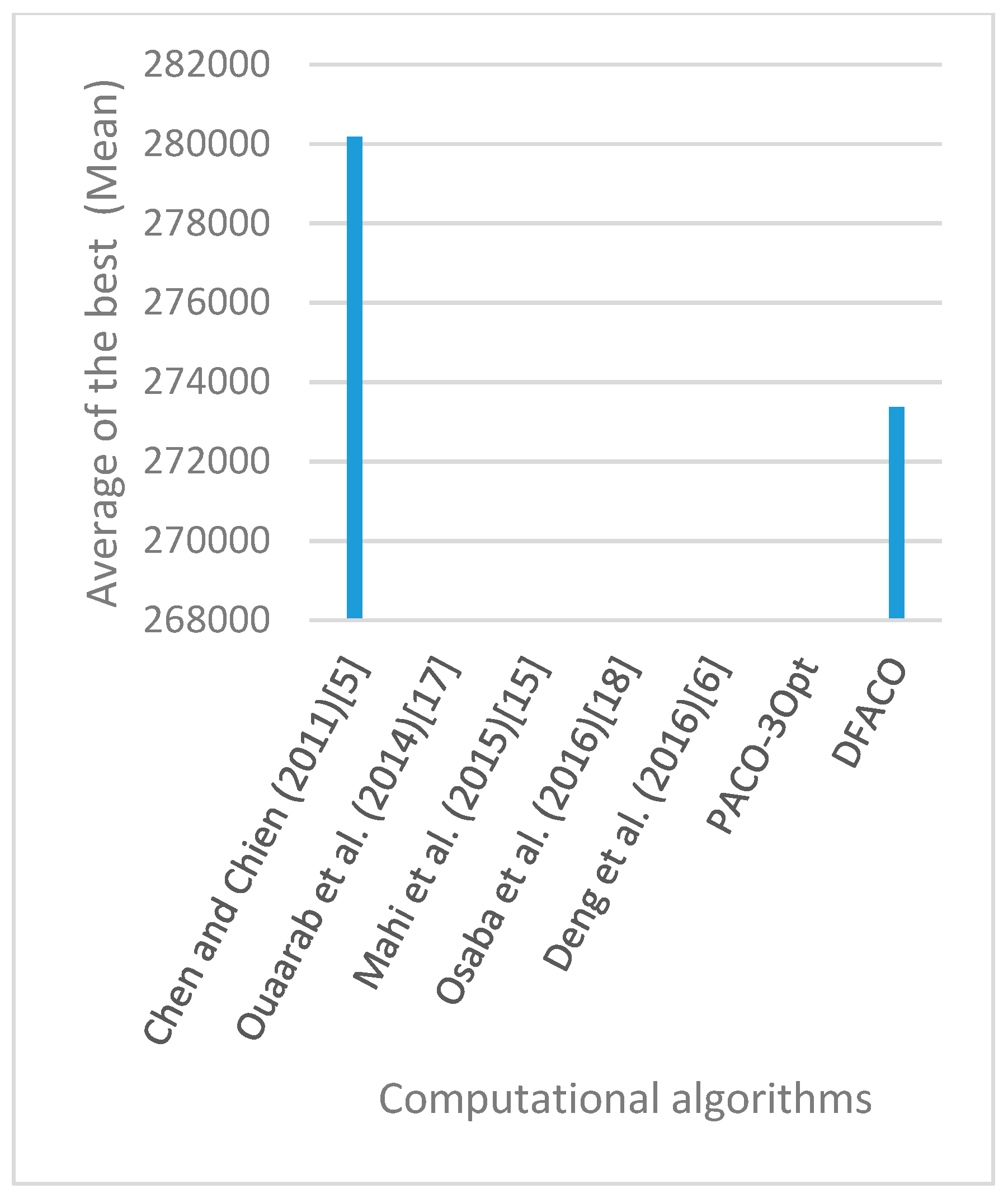
| rl1323 | 270,199 | 280,181.5 | 1761.7 | 277,642 | NA | NA | NA | NA | NA | NA | NA | NA | NA | NA | NA | NA | 273,367.9 | 484.8 | 272,487 |
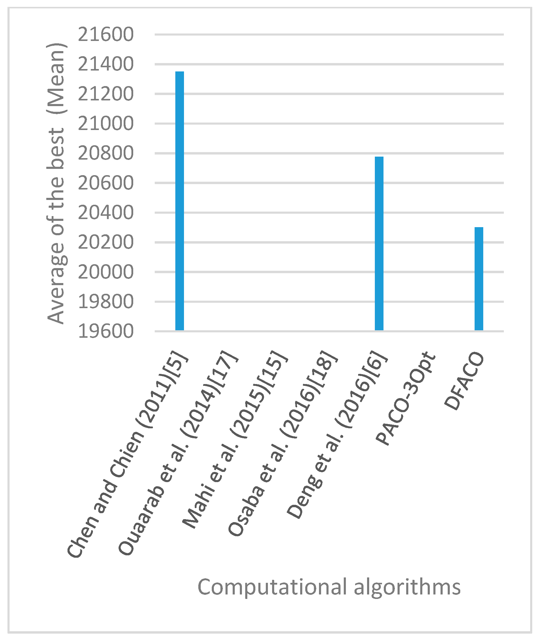
| fl1400 | 20,127 | 21,349.63 | 527.88 | 20,593 | NA | NA | NA | NA | NA | NA | NA | NA | NA | 20,776.2 | NA | 20,683.8 | 20,300.77 | 35.27 | 20,239 |
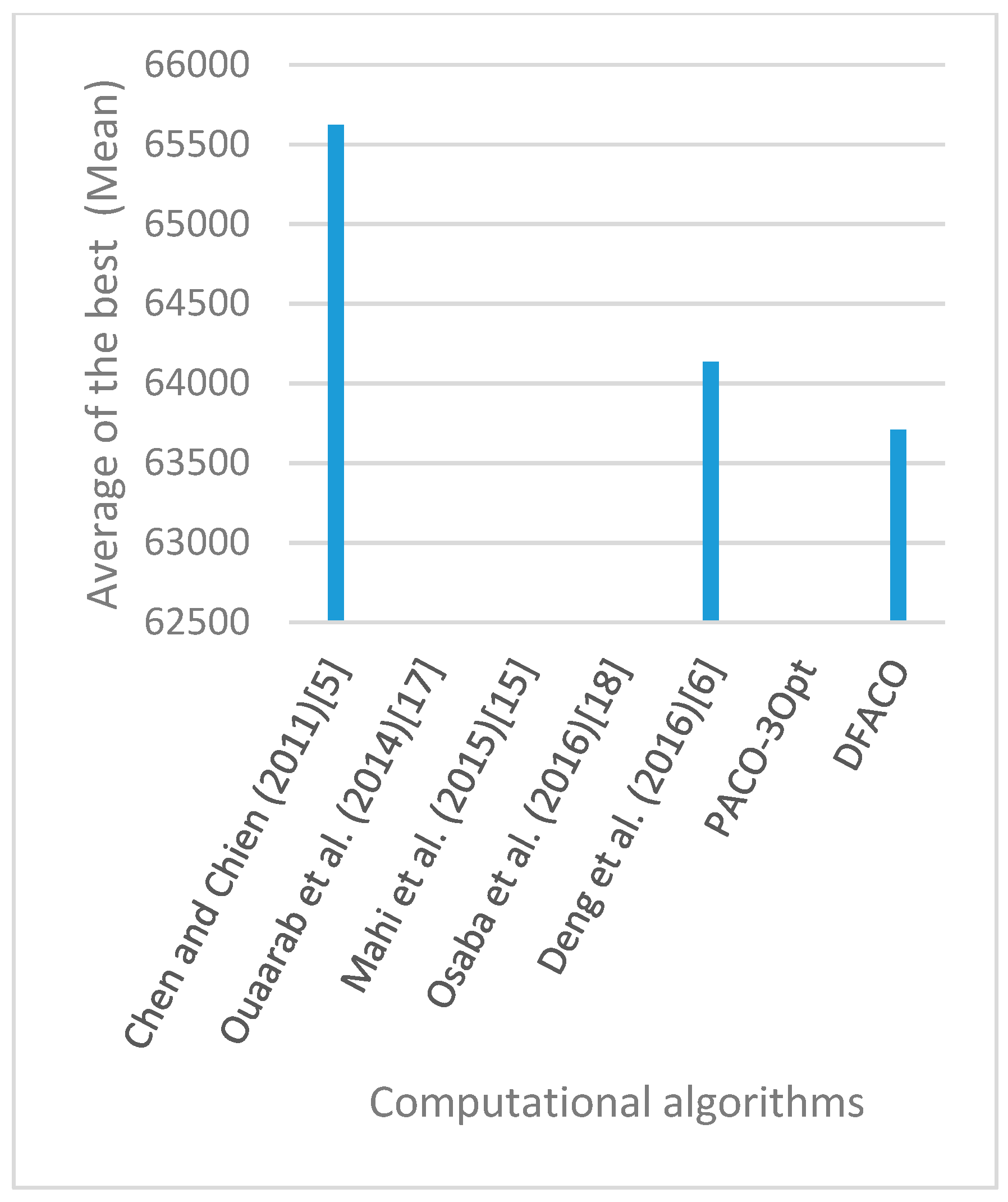
| d1655 | 62,128 | 65,621.13 | 1031.9 | 64,151 | NA | NA | NA | NA | NA | NA | NA | NA | NA | 64,133.7 | NA | 63,615.6 | 63,707.87 | 114.84 | 63,428.00 |
| TSP Instance | BKS | Chen and Chien (2011) [8] | Ouaarab et al. (2014) [20] | Mahi et al. (2015) [18] | Osaba et al. (2016) [21] | Deng et al. (2016) [9] | DFACO | ||||||
|---|---|---|---|---|---|---|---|---|---|---|---|---|---|
| PDav | PDbest | PDav | PDbest | PDav | PDbest | PDav | PDbest | PDav | PDbest | PDav | PDbest | ||
| eil51 | 426 | 0.30 | 0.23 | 0.00 | 0.00 | 0.11 | 0.00 | 0.49 | 0.00 | 0.28 | 0.00 | 0.00 | 0.00 |
| eil76 | 538 | 0.41 | 0.00 | 0.01 | 0.00 | 0.06 | 0.00 | 1.88 | 0.19 | 0.43 | 0.21 | 0.00 | 0.00 |
| eil101 | 629 | 0.99 | 0.16 | 0.23 | 0.00 | 0.59 | 0.32 | 2.77 | 0.79 | 0.90 | 0.16 | 0.00 | 0.00 |
| berlin52 | 7542 | 0.00 | 0.00 | 0.00 | 0.00 | 0.02 | 0.00 | 0.00 | 0.00 | NA | NA | 0.00 | 0.00 |
| bier127 | 118,282 | 0.96 | 0.00 | 0.07 | 0.00 | NA | NA | NA | NA | NA | NA | 0.00 | 0.00 |
| ch130 | 6110 | 1.57 | 0.51 | 0.42 | 0.00 | NA | NA | NA | NA | 0.23 | 0.05 | 0.00 | 0.00 |
| ch150 | 6528 | 0.55 | 0.00 | 0.34 | 0.00 | 0.55 | 0.00 | NA | NA | 0.18 | 0.00 | 0.00 | 0.00 |
| rd100 | 7910 | 0.98 | 0.00 | NA | NA | NA | NA | NA | NA | 0.31 | 0.00 | 0.00 | 0.00 |
| lin105 | 14,379 | 0.19 | 0.00 | 0.00 | 0.00 | 0.00 | 0.00 | NA | NA | 0.11 | 0.02 | 0.00 | 0.00 |
| lin318 | 42,029 | 2.32 | 1.09 | 0.97 | 0.23 | NA | NA | NA | NA | 0.81 | 0.61 | 0.47 | 0.22 |
| kroA100 | 21,282 | 0.42 | 0.00 | 0.00 | 0.00 | 0.77 | 0.09 | 0.77 | 0.00 | NA | NA | 0.00 | 0.00 |
| kroA150 | 26,524 | 1.41 | 0.00 | 0.17 | 0.00 | NA | NA | NA | NA | NA | NA | 0.00 | 0.00 |
| kroA200 | 29,368 | 1.26 | 0.05 | 0.27 | 0.05 | 0.95 | 0.34 | NA | NA | 0.23 | 0.04 | d0.00 | 0.00 |
| kroB100 | 22,141 | 0.64 | 0.00 | 0.00 | 0.00 | NA | NA | 1.65 | 0.00 | NA | NA | 0.00 | 0.00 |
| kroB150 | 26,130 | 1.22 | 0.00 | 0.11 | 0.00 | NA | NA | NA | NA | 0.17 | 0.04 | 0.00 | 0.00 |
| kroB200 | 29,437 | 2.03 | 0.35 | 0.36 | 0.04 | NA | NA | NA | NA | 0.26 | 0.22 | 0.02 | 0.00 |
| kroC100 | 20,749 | 0.63 | 0.00 | 0.00 | 0.00 | NA | NA | 1.45 | 0.00 | NA | NA | 0.00 | 0.00 |
| kroD100 | 21,294 | 1.53 | 0.07 | 0.05 | 0.00 | NA | NA | 1.41 | 0.00 | NA | NA | 0.00 | 0.00 |
| kroE100 | 22,068 | 0.52 | 0.00 | 0.06 | 0.00 | NA | NA | 1.28 | 0.00 | NA | NA | 0.00 | 0.00 |
| rat575 | 6773 | 2.38 | 1.74 | NA | NA | NA | NA | NA | NA | 1.89 | 1.28 | −5.85 | −6.19 |
| rat783 | 8806 | 3.10 | 2.07 | NA | NA | NA | NA | NA | NA | 1.94 | 1.53 | 19.30 | 19.01 |
| rl1323 | 270,199 | 3.69 | 2.75 | NA | NA | NA | NA | NA | NA | NA | NA | 1.17 | 0.85 |
| fl1400 | 20,127 | 6.07 | 2.32 | NA | NA | NA | NA | NA | NA | 3.23 | 2.77 | 0.86 | 0.56 |
| d1655 | 62,128 | 5.62 | 3.26 | NA | NA | NA | NA | NA | NA | 3.23 | 2.39 | 2.38 | 2.02 |
© 2019 by the authors. Licensee MDPI, Basel, Switzerland. This article is an open access article distributed under the terms and conditions of the Creative Commons Attribution (CC BY) license (http://creativecommons.org/licenses/by/4.0/).
Share and Cite
Dahan, F.; El Hindi, K.; Mathkour, H.; AlSalman, H. Dynamic Flying Ant Colony Optimization (DFACO) for Solving the Traveling Salesman Problem. Sensors 2019, 19, 1837. https://doi.org/10.3390/s19081837
Dahan F, El Hindi K, Mathkour H, AlSalman H. Dynamic Flying Ant Colony Optimization (DFACO) for Solving the Traveling Salesman Problem. Sensors. 2019; 19(8):1837. https://doi.org/10.3390/s19081837
Chicago/Turabian StyleDahan, Fadl, Khalil El Hindi, Hassan Mathkour, and Hussien AlSalman. 2019. "Dynamic Flying Ant Colony Optimization (DFACO) for Solving the Traveling Salesman Problem" Sensors 19, no. 8: 1837. https://doi.org/10.3390/s19081837
APA StyleDahan, F., El Hindi, K., Mathkour, H., & AlSalman, H. (2019). Dynamic Flying Ant Colony Optimization (DFACO) for Solving the Traveling Salesman Problem. Sensors, 19(8), 1837. https://doi.org/10.3390/s19081837