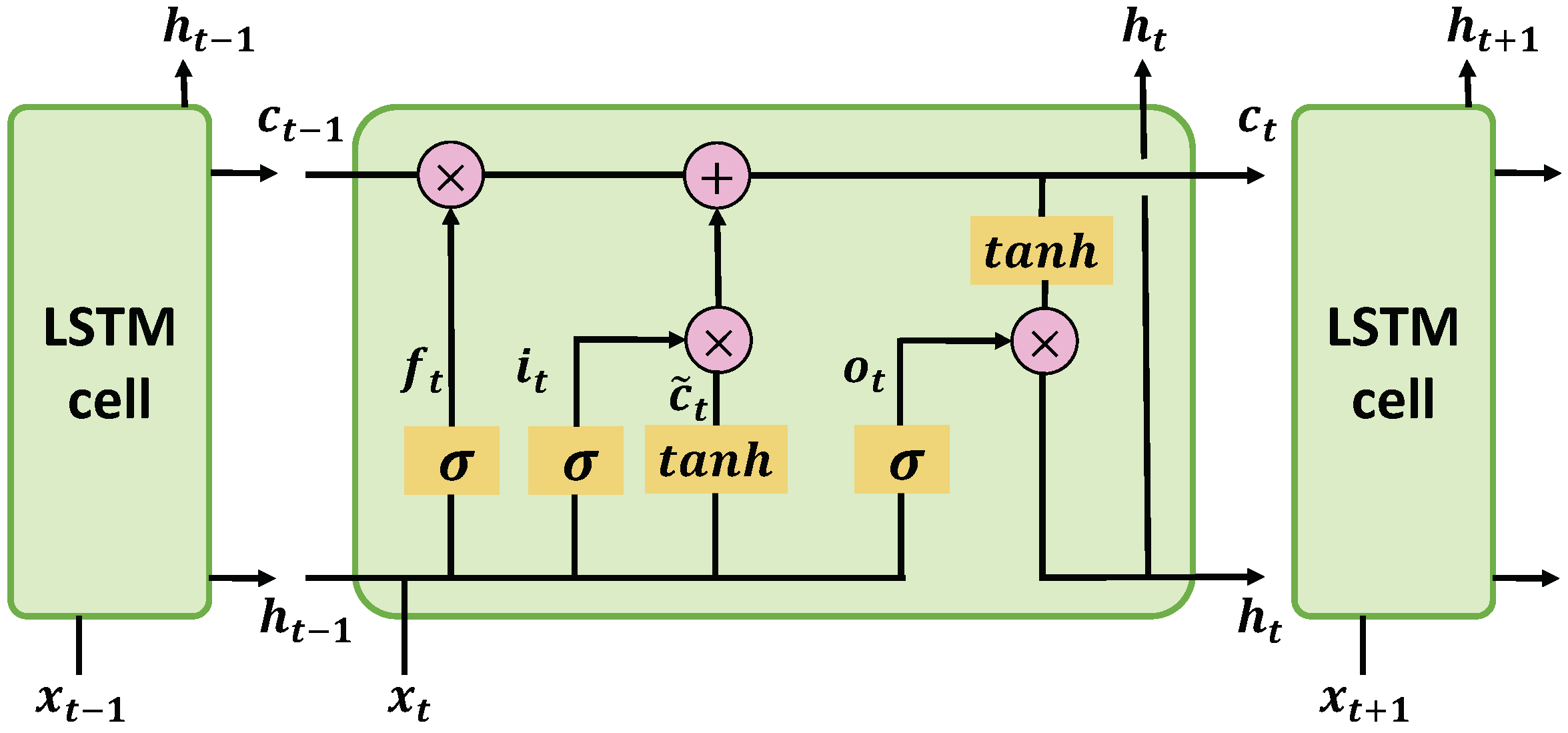
Figure 1.
A basic cell of LSTM. By explicitly introducing a memory cell ct together with some control gates ft, it and ot to decide the information flow, LSTM can capture long-term dependencies of the sequential inputs.
Figure 1.
A basic cell of LSTM. By explicitly introducing a memory cell ct together with some control gates ft, it and ot to decide the information flow, LSTM can capture long-term dependencies of the sequential inputs.
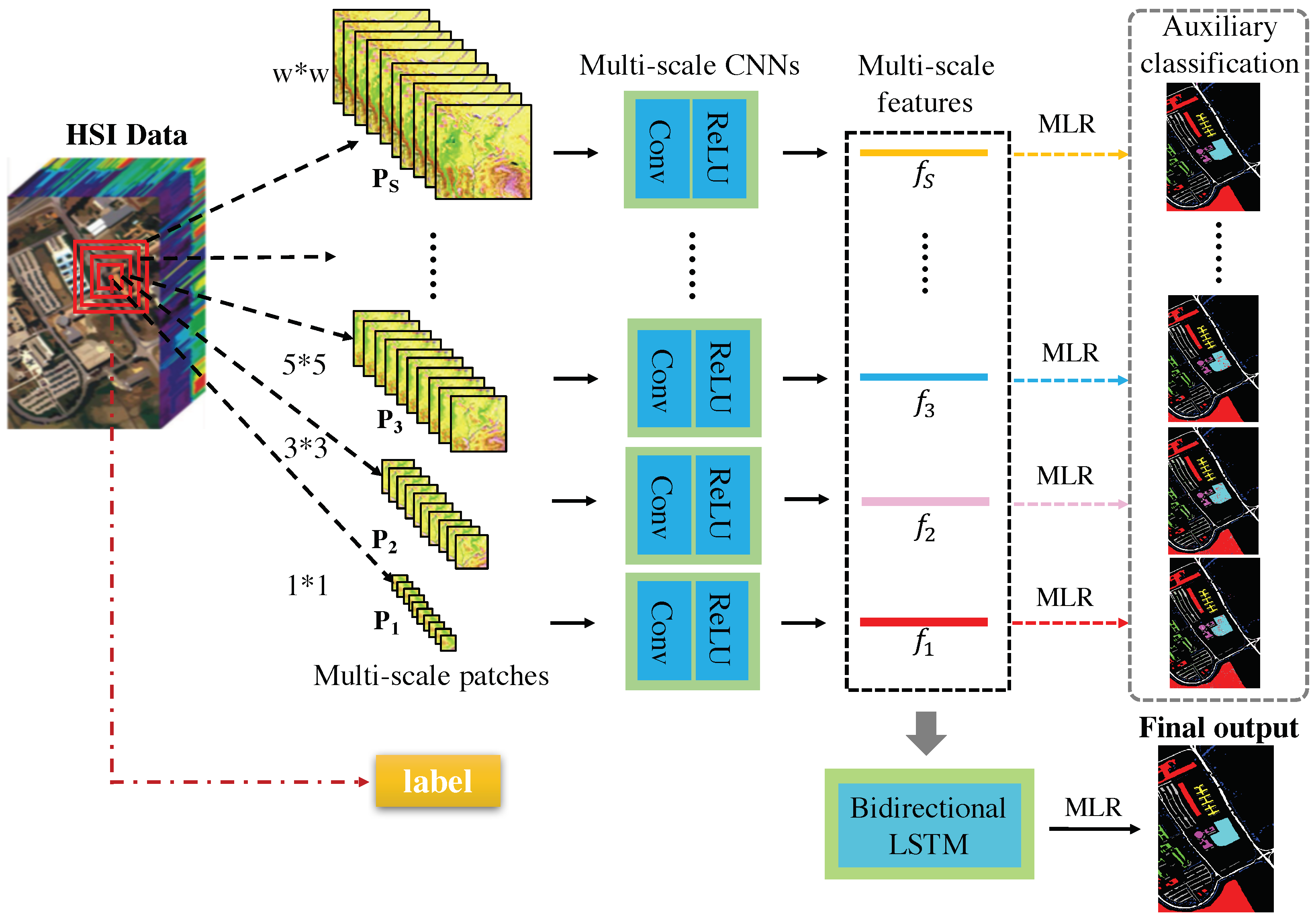
Figure 2.
The architecture of the proposed HMCNN-AC consisting of multi-scale CNNs and a bidirectional LSTM. For each pixel in HSI, the generated multi-scale patches are sent to the multi-scale CNNs with auxiliary classifiers to extract multi-scale spectral–spatial features, then a bidirectional LSTM is employed to explore the scale-dependency of multi-scale features and output a hierarchical representation for the final supervised classification.
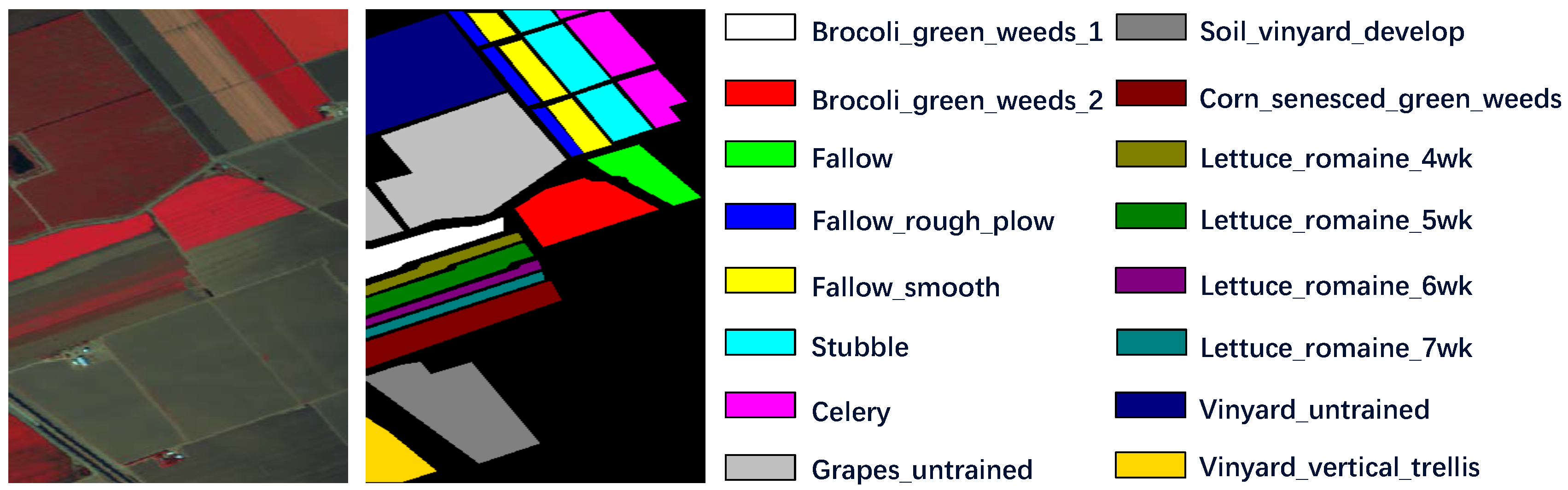
Figure 3.
Salinas dataset description. The false-color image is generated from spectral band 52, 25, 10 and the groundtruth map together with the respective classes are displayed.
Figure 3.
Salinas dataset description. The false-color image is generated from spectral band 52, 25, 10 and the groundtruth map together with the respective classes are displayed.
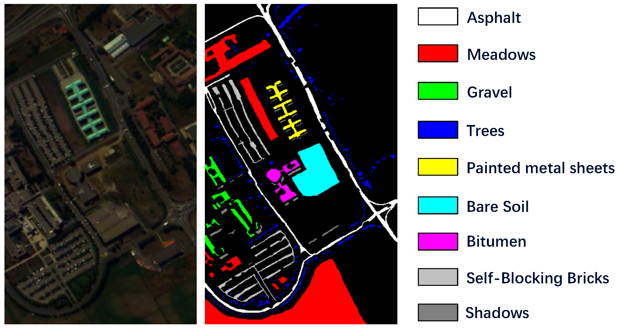
Figure 4.
PaviaU dataset description. The false-color image is generated from spectral band 56, 28, 5 and the ground truth map together with the respective classes are displayed.
Figure 4.
PaviaU dataset description. The false-color image is generated from spectral band 56, 28, 5 and the ground truth map together with the respective classes are displayed.
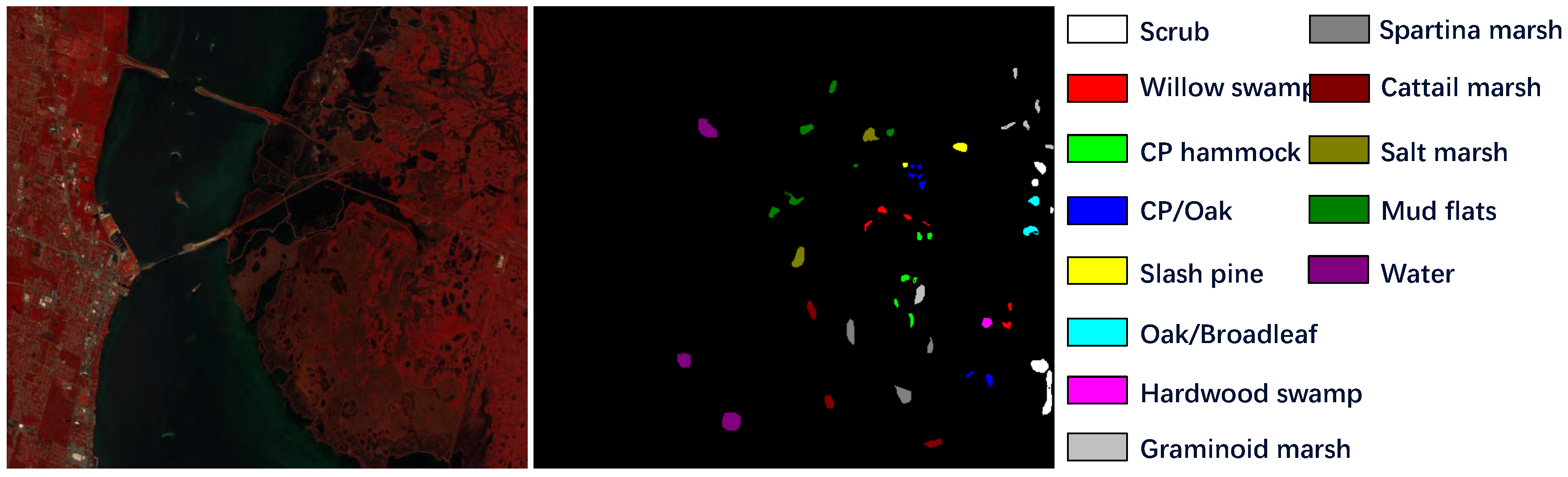
Figure 5.
KSC dataset description. The false-color image is generated from spectral band 56, 28, 5 and the ground truth map together with the respective classes are displayed.
Figure 5.
KSC dataset description. The false-color image is generated from spectral band 56, 28, 5 and the ground truth map together with the respective classes are displayed.
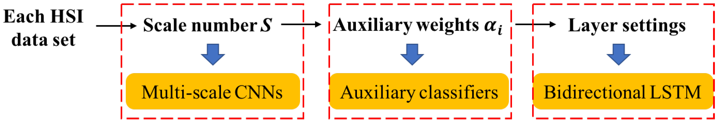
Figure 6.
The flow chart of hyperparameter tuning process. For each HSI, we first fix auxiliary weights αi and layer settings in Bi-LSTM, and adjust the input scale number S to find the optimal one. Then we fix scale number S and layer settings in Bi-LSTM to find suitable auxiliary weights αi. The same procedure goes for determining suitable layer settings in Bi-LSTM. Finally, we obtain all the determined hyperparameters.
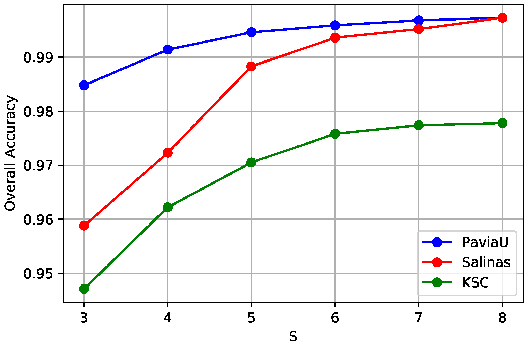
Figure 7.
The curves of OA obtained by different input scale numbers S for three HSI datasets. The OAs first arise with the increase of the input scale number S, and then become saturated for all three HSIs. Thus, we choose the scale number S = 8 for all the HSIs for our proposed framework.
Figure 7.
The curves of OA obtained by different input scale numbers S for three HSI datasets. The OAs first arise with the increase of the input scale number S, and then become saturated for all three HSIs. Thus, we choose the scale number S = 8 for all the HSIs for our proposed framework.
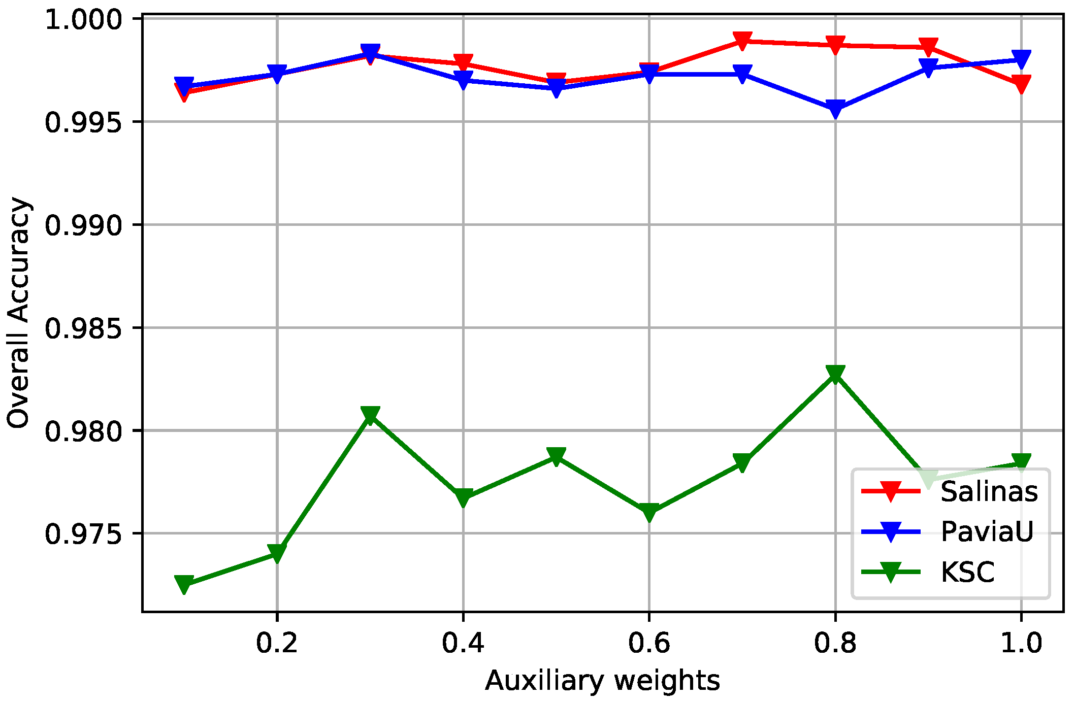
Figure 8.
The curves of OA obtained by different multi-scale auxiliary weights for three HSI datasets. The auxiliary weights are set from 0.1 to 1, with an increment of 0.1. The optimal α is determined corresponding to the highest OA value for each HSI.
Figure 8.
The curves of OA obtained by different multi-scale auxiliary weights for three HSI datasets. The auxiliary weights are set from 0.1 to 1, with an increment of 0.1. The optimal α is determined corresponding to the highest OA value for each HSI.
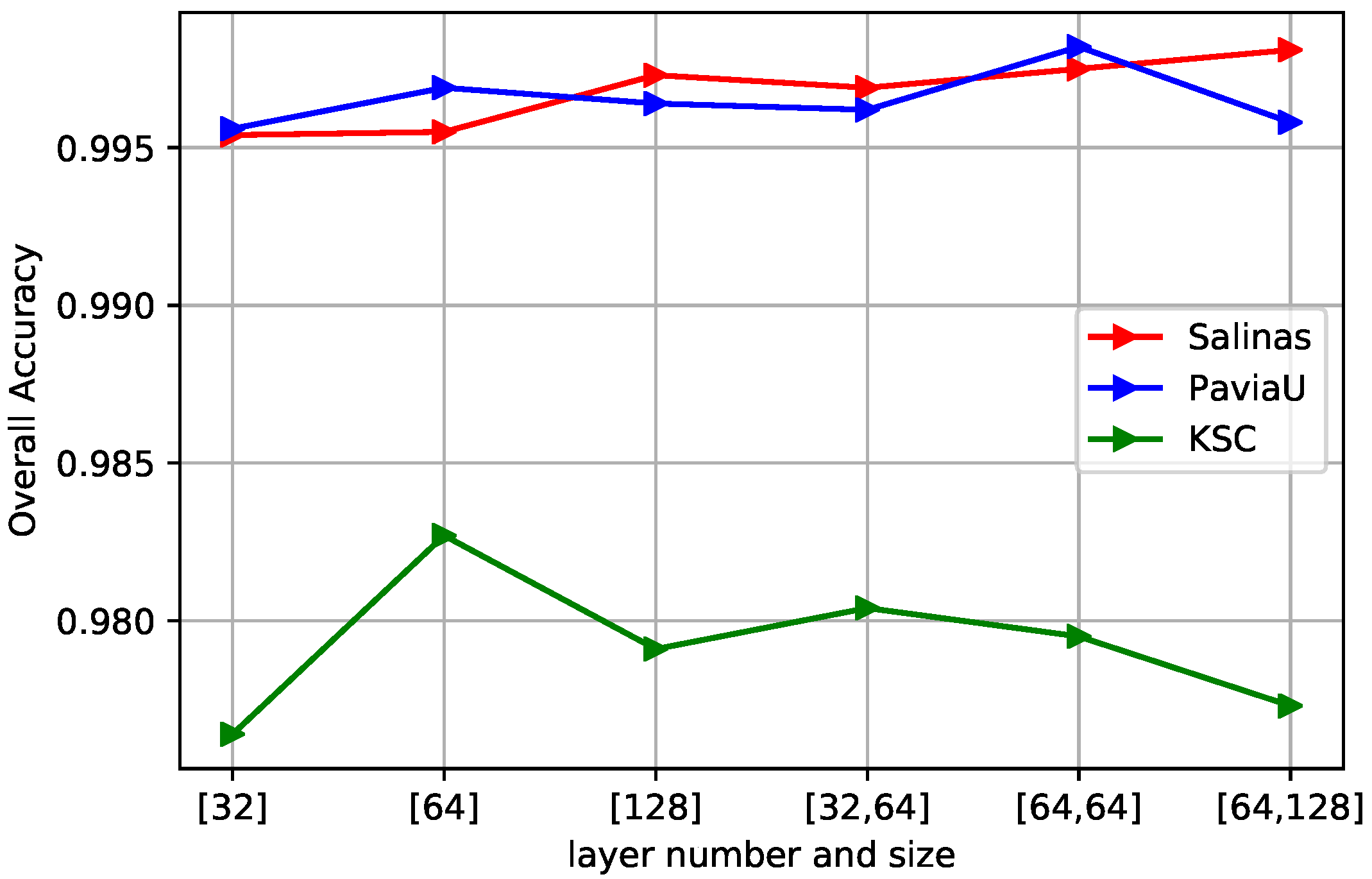
Figure 9.
The curves of OA obtained by different layer numbers and hidden units in bidirectional LSTM. The optimal hyperparameter choice for Salinas is two-layer with 64 and 128 hidden units respectively, two-layer with 64 and 64 units for PaviaU, and one-layer with 64 hidden units for KSC due to smaller data size.
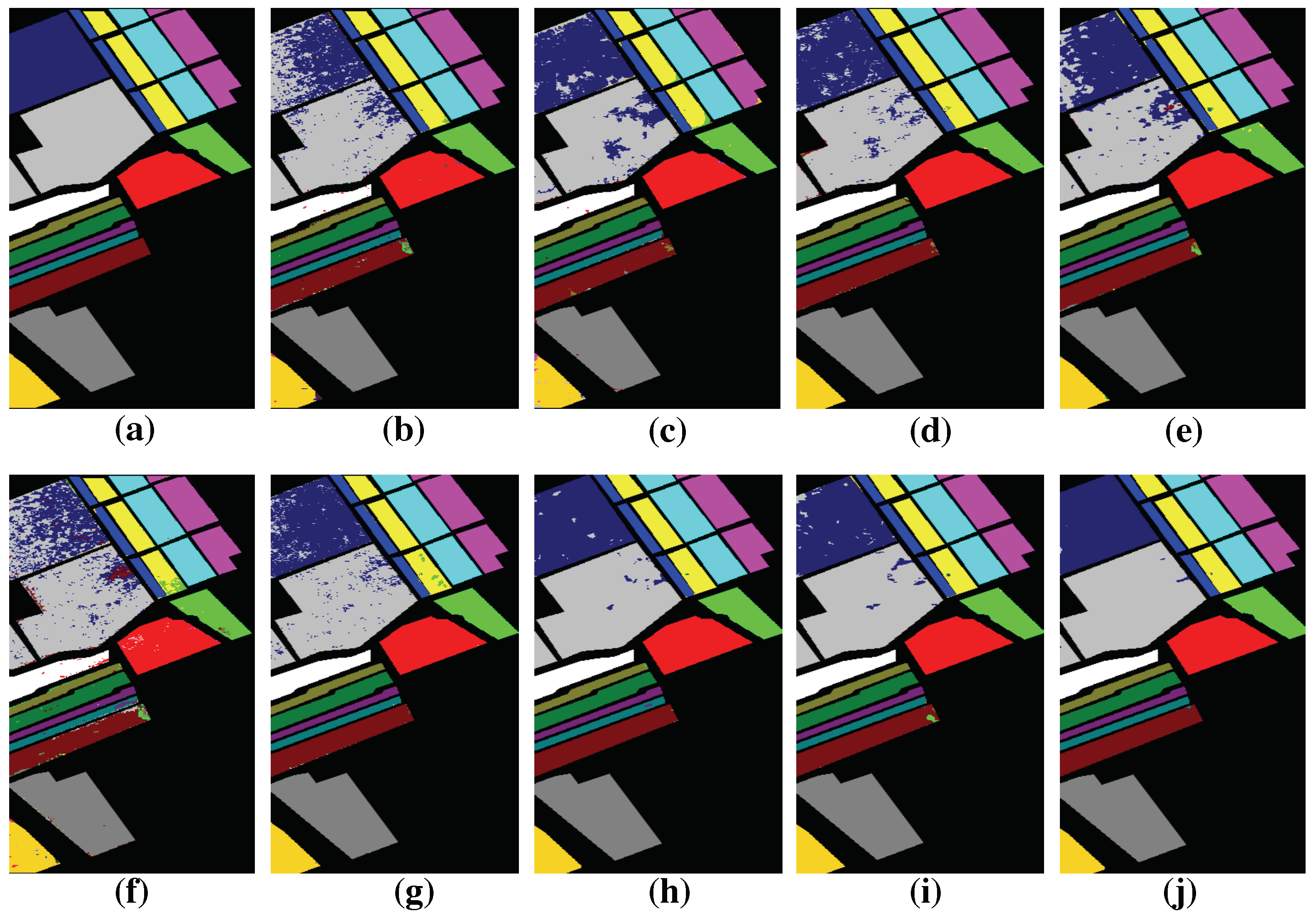
Figure 10.
Groundtruth and classification maps with 5% training samples from Salinas dataset. (a) Groundtruth; (b) SVM; (c) EMP-SVM; (d) SAE-LR; (e) CNN-MLR; (f) LSTM; (g) MCNN; (h) HMCNN; (i) MCNN-AC; and (j) HMCNN-AC. The proposed HMCNN-AC yields the cleanest visualization maps with improved spatial consistency, which is most similar to the groundtruth map.
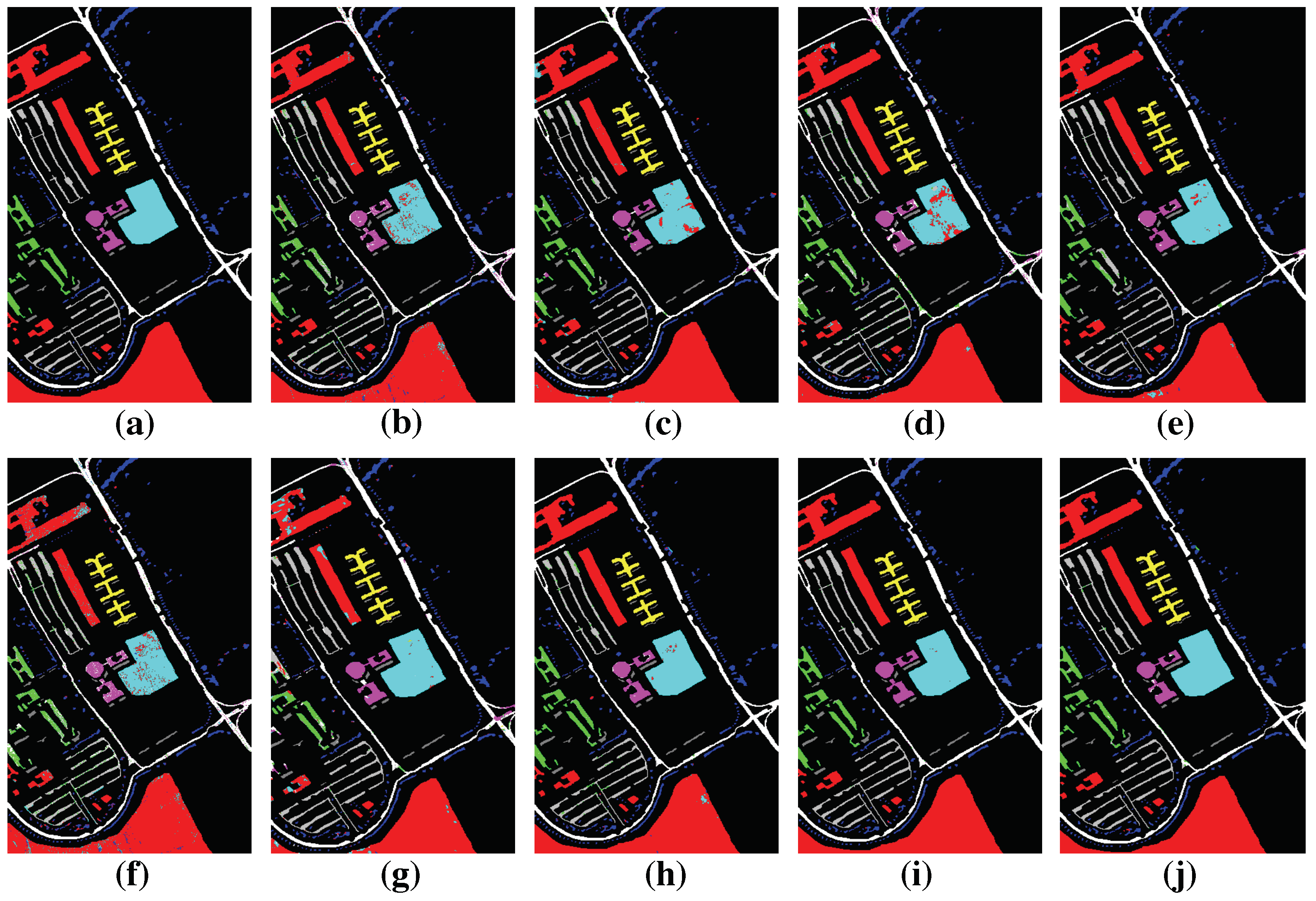
Figure 11.
Groundtruth and Classification maps with 5% training samples from PaviaU dataset. (a) Groundtruth; (b) SVM; (c) EMP-SVM; (d) SAE-LR; (e) CNN-MLR; (f) LSTM; (g) MCNN; (h) HMCNN; (i) MCNN-AC; and (j) HMCNN-AC. The proposed HMCNN-AC yields the cleanest visualization maps with improved spatial consistency, which is most similar to the groundtruth map.
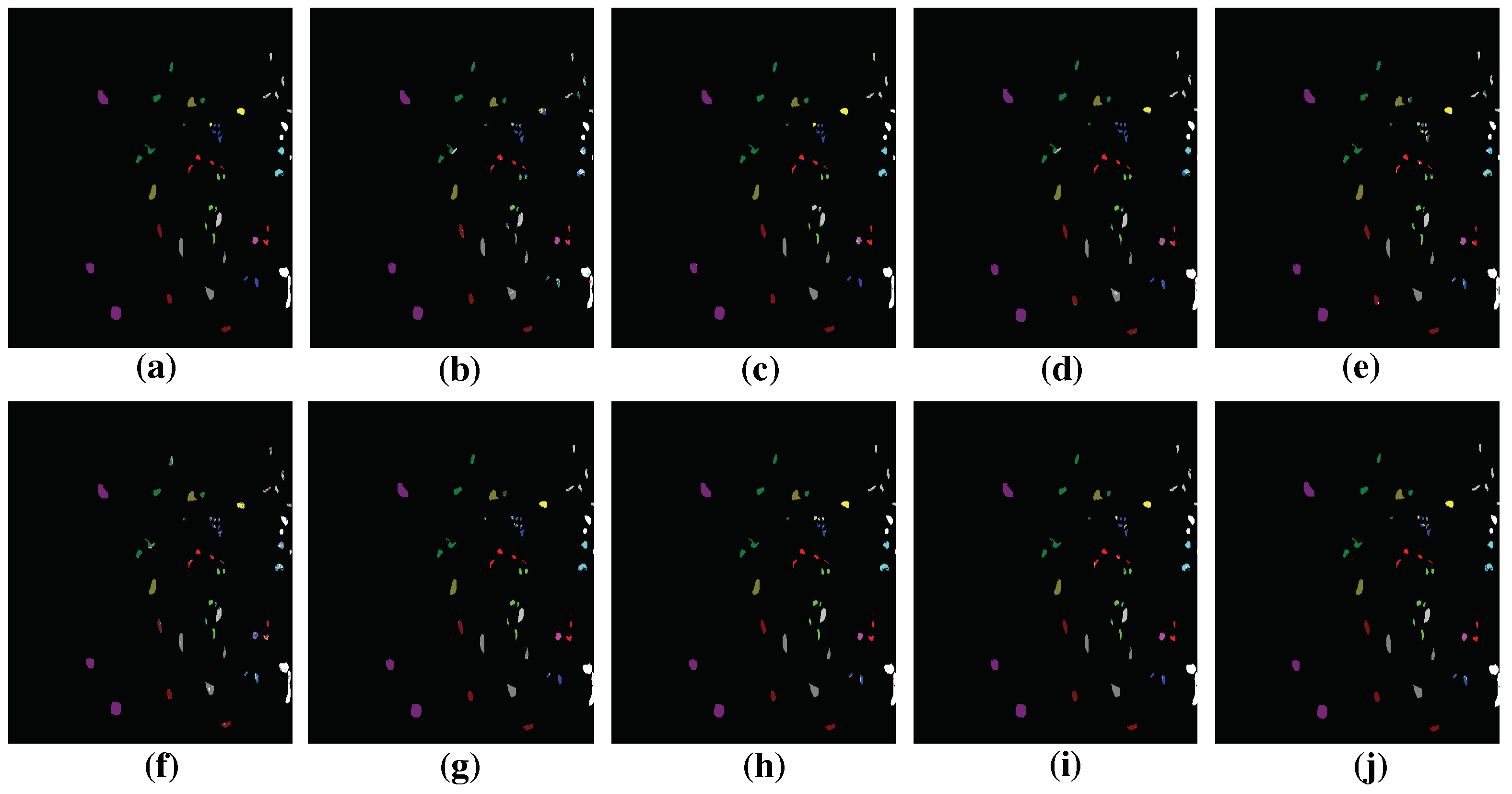
Figure 12.
Groundtruth and Classification maps with 10% training samples from KSC dataset. (a) Ground truth; (b) SVM; (c) EMP-SVM; (d) SAE-LR; (e) CNN-MLR; (f) LSTM; (g) MCNN; (h) HMCNN; (i) MCNN-AC; and (j) HMCNN-AC. The proposed HMCNN-AC yields the cleanest visualization maps with improved spatial consistency, which is most similar to the groundtruth map.
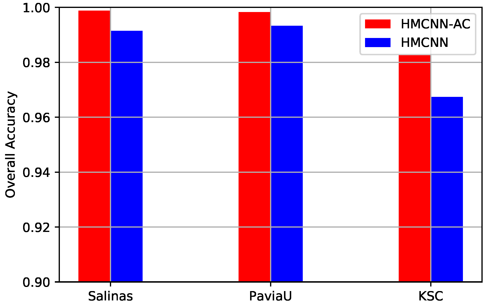
Figure 13.
OAs comparison of HMCNN and HMCNN-AC on three datasets for effective analysis of auxiliary classifiers. For all three HSIs, OA value decreases for the constructed HMCNN framework, which confirms the effectiveness of the adopted auxiliary classifiers.
Figure 13.
OAs comparison of HMCNN and HMCNN-AC on three datasets for effective analysis of auxiliary classifiers. For all three HSIs, OA value decreases for the constructed HMCNN framework, which confirms the effectiveness of the adopted auxiliary classifiers.
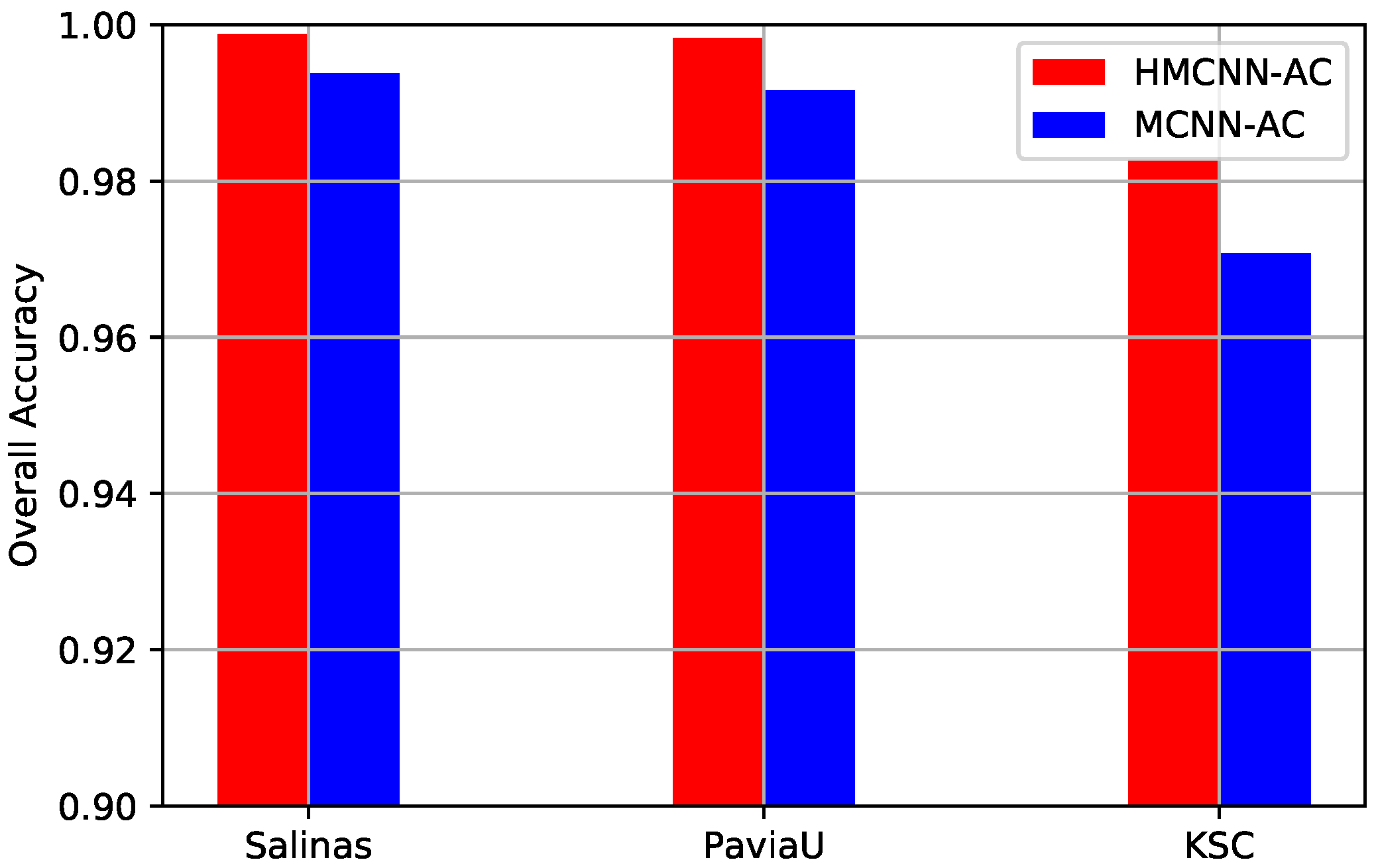
Figure 14.
OAs comparison of the proposed MCNN-AC and HMCNN-AC on three datasets for effective analysis of bidirectional LSTM. For all three HSIs, OA value decreases for the constructed MCNN-AC framework, which validates the effectiveness of the adopted bidirectional LSTM.
Figure 14.
OAs comparison of the proposed MCNN-AC and HMCNN-AC on three datasets for effective analysis of bidirectional LSTM. For all three HSIs, OA value decreases for the constructed MCNN-AC framework, which validates the effectiveness of the adopted bidirectional LSTM.
Table 1.
The network architectures of multi-scale CNNs. For multi-scale input patches with various input scales, the detailed structures of each sub-network including the numbers of convolution layers, kernel sizes and kernel numbers are specified.
Table 1.
The network architectures of multi-scale CNNs. For multi-scale input patches with various input scales, the detailed structures of each sub-network including the numbers of convolution layers, kernel sizes and kernel numbers are specified.
| Layer No. | P1 (1 × 1) | P2 (3 × 3) | P3 (5 × 5) | P4 (7 × 7) | P5 (9 × 9) | P6 (11 × 11) | P7 (13 × 13) | P8 (15 × 15) |
|---|
| 1 | 1 × 1 × 32 | 1 × 1 × 32 | 3 × 3 × 32 | 3 × 3 × 32 | 3 × 3 × 32 | 3 × 3 × 32 | 3 × 3 × 32 | 3 × 3 × 32 |
| 2 | 1 × 1 × 32 | 3 × 3 × 32 | 3 × 3 × 32 | 3 × 3 × 32 | 3 × 3 × 32 | 3 × 3 × 32 | 3 × 3 × 32 | 5 × 5 × 32 |
| 3 | | | | 3 × 3 × 64 | 5 × 5 × 64 | 3 × 3 × 64 | 5 × 5 × 32 | 5 × 5 × 64 |
| 4 | | | | | | 5 × 5 × 64 | 5 × 5 × 64 | 5 × 5 × 64 |
Table 2.
Groundtruth classes for Salinas scene and the corresponding number of training samples and testing samples for classification experiments.
Table 2.
Groundtruth classes for Salinas scene and the corresponding number of training samples and testing samples for classification experiments.
| Class Number | Class Name | Train | Test |
|---|
| 1 | Brocoli green weeds 1 | 100 | 1909 |
| 2 | Brocoli green weeds 2 | 186 | 3540 |
| 3 | Fallow | 99 | 1877 |
| 4 | Fallow rough plow | 70 | 1324 |
| 5 | Fallow smooth | 134 | 2544 |
| 6 | Stubble | 198 | 3761 |
| 7 | Celery | 179 | 3400 |
| 8 | Grapes untrained | 563 | 10,708 |
| 9 | Soil vinyard develop | 310 | 5893 |
| 10 | Corn senesced green weeds | 164 | 3114 |
| 11 | Lettuce romaine 4 wk | 53 | 1015 |
| 12 | Lettuce romaine 5 wk | 96 | 1831 |
| 13 | Lettuce romaine 6 wk | 46 | 870 |
| 14 | Lettuce romaine 7 wk | 54 | 1016 |
| 15 | Vinyard untrained | 363 | 6905 |
| 16 | Vinyard vertical trellis | 90 | 1717 |
| total | | 2705 | 51,424 |
Table 3.
Groundtruth classes for PaviaU scene and the corresponding number of training samples and testing samples for classification experiments.
Table 3.
Groundtruth classes for PaviaU scene and the corresponding number of training samples and testing samples for classification experiments.
| Class Number | Class Name | Train | Test |
|---|
| 1 | Asphalt | 331 | 6300 |
| 2 | Meadows | 932 | 17,717 |
| 3 | Gravel | 105 | 1994 |
| 4 | Trees | 153 | 2911 |
| 5 | Painted metal sheets | 67 | 1278 |
| 6 | Bare Soil | 251 | 4778 |
| 7 | Bitumen | 66 | 1264 |
| 8 | Self-Blocking Bricks | 184 | 3498 |
| 9 | Shadows | 47 | 900 |
| total | | 2136 | 40,640 |
Table 4.
Groundtruth classes for KSC scene and the corresponding number of training samples and testing samples for classification experiments.
Table 4.
Groundtruth classes for KSC scene and the corresponding number of training samples and testing samples for classification experiments.
| Class Number | Class Name | Train | Test |
|---|
| 1 | Scrub | 76 | 685 |
| 2 | Willow swamp | 24 | 219 |
| 3 | Cabbage palm hummock | 26 | 230 |
| 4 | Cabbage/oak hummock | 25 | 227 |
| 5 | Slash pine | 16 | 145 |
| 6 | Oak/broadleaf hummock | 23 | 206 |
| 7 | Hardwood swamp | 11 | 94 |
| 8 | Graminoid marsh | 43 | 388 |
| 9 | Spartina marsh | 52 | 468 |
| 10 | Cattail marsh | 40 | 364 |
| 11 | Salt marsh | 42 | 377 |
| 12 | Mud flats | 50 | 453 |
| 13 | Water | 93 | 834 |
| total | | 521 | 4690 |
Table 5.
Classification accuracy (%) for Salinas dataset using 5% training samples via different classification algorithms. The three proposed frameworks HMCNN, MCNN-AC and HMCNN-AC outperform other baseline methods in results.
Table 5.
Classification accuracy (%) for Salinas dataset using 5% training samples via different classification algorithms. The three proposed frameworks HMCNN, MCNN-AC and HMCNN-AC outperform other baseline methods in results.
| Class No. | SVM | EMP-SVM | SAE-PCA | CNN-MLR | LSTM | MCNN | HMCNN | MCNN-AC | HMCNN-AC |
|---|
| 1 | 98.11 | 99.27 | 100.00 | 100.00 | 96.51 | 100.00 | 100.00 | 100.00 | 100.00 |
| 2 | 99.52 | 99.49 | 99.91 | 99.93 | 98.31 | 98.64 | 100.00 | 100.00 | 100.00 |
| 3 | 99.68 | 99.52 | 99.09 | 98.68 | 97.22 | 96.84 | 99.85 | 100.00 | 99.90 |
| 4 | 99.17 | 98.56 | 98.17 | 97.99 | 98.71 | 97.49 | 99.49 | 99.71 | 100.00 |
| 5 | 97.27 | 94.46 | 100.00 | 99.28 | 91.78 | 98.47 | 99.59 | 99.77 | 99.81 |
| 6 | 98.36 | 99.81 | 99.82 | 99.75 | 99.62 | 100.00 | 100.00 | 100.00 | 100.00 |
| 7 | 98.67 | 98.59 | 93.26 | 99.94 | 99.36 | 100.00 | 100.00 | 100.00 | 100.00 |
| 8 | 91.52 | 88.61 | 92.81 | 89.36 | 88.36 | 94.03 | 98.00 | 98.53 | 99.86 |
| 9 | 98.96 | 99.56 | 99.74 | 100.00 | 98.63 | 99.93 | 100.00 | 100.00 | 100.00 |
| 10 | 94.09 | 96.56 | 96.35 | 96.18 | 89.51 | 99.31 | 97.94 | 99.78 | 99.32 |
| 11 | 90.24 | 98.91 | 94.42 | 99.04 | 91.67 | 99.83 | 100.00 | 98.92 | 100.00 |
| 12 | 99.19 | 99.78 | 99.88 | 100.00 | 99.12 | 99.56 | 100.00 | 100.00 | 100.00 |
| 13 | 98.85 | 98.27 | 99.54 | 99.81 | 98.36 | 100.00 | 100.00 | 99.88 | 100.00 |
| 14 | 97.93 | 95.96 | 98.99 | 99.14 | 89.81 | 99.32 | 98.35 | 98.73 | 100.00 |
| 15 | 68.15 | 89.09 | 91.62 | 84.26 | 55.71 | 97.23 | 96.12 | 98.34 | 99.74 |
| 16 | 96.62 | 94.52 | 96.96 | 98.72 | 96.46 | 99.21 | 100.00 | 99.85 | 100.00 |
| OA (%) | 92.33 | 95.08 | 95.69 | 95.22 | 89.37 | 97.73 | 99.14 | 99.38 | 99.88 |
| AA (%) | 93.47 | 96.93 | 96.32 | 96.56 | 93.07 | 98.69 | 99.14 | 99.59 | 99.91 |
| Kappa | 0.9144 | 0.9453 | 0.9520 | 0.9470 | 0.8821 | 0.9742 | 0.9875 | 0.9932 | 0.9987 |
Table 6.
Classification accuracy (%) for PaviaU dataset using 5% training samples via different classification algorithms. The three proposed frameworks HMCNN, MCNN-AC and HMCNN-AC outperform other baseline methods in results.
Table 6.
Classification accuracy (%) for PaviaU dataset using 5% training samples via different classification algorithms. The three proposed frameworks HMCNN, MCNN-AC and HMCNN-AC outperform other baseline methods in results.
| Class No. | SVM | EMP-SVM | SAE-PCA | CNN-MLR | LSTM | MCNN | HMCNN | MCNN-AC | HMCNN-AC |
|---|
| 1 | 92.30 | 97.44 | 90.55 | 98.33 | 93.36 | 95.27 | 98.63 | 99.12 | 99.68 |
| 2 | 98.00 | 98.08 | 98.95 | 98.94 | 94.97 | 98.73 | 99.99 | 99.95 | 100.00 |
| 3 | 74.07 | 93.03 | 92.34 | 73.63 | 69.37 | 92.21 | 97.55 | 93.75 | 98.72 |
| 4 | 94.47 | 97.39 | 98.91 | 98.81 | 94.12 | 99.60 | 98.67 | 98.15 | 99.73 |
| 5 | 99.06 | 99.37 | 100.00 | 99.63 | 99.14 | 99.75 | 100.00 | 100.00 | 100.00 |
| 6 | 87.94 | 92.42 | 84.47 | 97.30 | 88.23 | 94.50 | 100.00 | 99.98 | 100.00 |
| 7 | 86.38 | 93.90 | 87.42 | 96.92 | 81.13 | 97.01 | 96.69 | 98.57 | 99.40 |
| 8 | 91.02 | 96.62 | 87.56 | 98.13 | 82.29 | 95.89 | 99.15 | 98.10 | 99.67 |
| 9 | 99.67 | 100.00 | 97.56 | 99.89 | 100.00 | 100.00 | 100.00 | 99.89 | 100.00 |
| OA (%) | 92.61 | 96.85 | 94.13 | 97.24 | 91.16 | 96.96 | 99.33 | 99.16 | 99.83 |
| AA (%) | 91.43 | 96.47 | 93.08 | 95.76 | 89.23 | 96.93 | 98.96 | 98.61 | 99.69 |
| Kappa | 0.9150 | 0.9582 | 0.9230 | 0.9647 | 0.8854 | 0.9625 | 0.9919 | 0.9893 | 0.9976 |
Table 7.
Classification accuracy (%) for KSC dataset using 10% training samples via different classification algorithms. The three proposed frameworks HMCNN, MCNN-AC and HMCNN-AC outperform other baseline methods in results.
Table 7.
Classification accuracy (%) for KSC dataset using 10% training samples via different classification algorithms. The three proposed frameworks HMCNN, MCNN-AC and HMCNN-AC outperform other baseline methods in results.
| Class No. | SVM | EMP-SVM | SAE-PCA | CNN-MLR | LSTM | MCNN | HMCNN | MCNN-AC | HMCNN-AC |
|---|
| 1 | 95.46 | 100.00 | 99.07 | 98.54 | 91.85 | 95.66 | 100.00 | 100.00 | 100.00 |
| 2 | 82.56 | 100.00 | 81.48 | 97.53 | 75.31 | 99.17 | 98.35 | 99.59 | 99.76 |
| 3 | 90.00 | 66.67 | 96.48 | 91.41 | 86.33 | 98.05 | 95.31 | 98.04 | 99.22 |
| 4 | 46.46 | 99.56 | 66.26 | 58.73 | 63.89 | 78.97 | 82.14 | 74.60 | 88.97 |
| 5 | 46.52 | 78.95 | 53.42 | 76.40 | 57.14 | 82.61 | 90.06 | 80.12 | 93.17 |
| 6 | 50.48 | 79.89 | 60.70 | 81.66 | 48.91 | 91.27 | 91.26 | 95.63 | 88.21 |
| 7 | 93.61 | 100.00 | 99.05 | 95.24 | 30.48 | 100.00 | 100.00 | 97.14 | 100.00 |
| 8 | 88.63 | 97.10 | 94.56 | 98.35 | 72.85 | 92.10 | 94.81 | 98.76 | 98.27 |
| 9 | 98.71 | 100.00 | 100.00 | 100.00 | 92.12 | 99.42 | 99.61 | 100.00 | 100.00 |
| 10 | 93.38 | 98.35 | 97.52 | 96.04 | 79.21 | 99.75 | 96.53 | 99.75 | 99.85 |
| 11 | 96.02 | 99.21 | 98.09 | 100.00 | 98.57 | 100.00 | 100.00 | 100.00 | 100.00 |
| 12 | 77.87 | 98.89 | 97.42 | 92.64 | 81.91 | 99.60 | 97.41 | 97.81 | 98.61 |
| 13 | 97.60 | 99.64 | 99.46 | 99.89 | 99.68 | 100.00 | 100.00 | 100.00 | 100.00 |
| OA (%) | 86.40 | 95.36 | 92.07 | 93.82 | 82.98 | 97.06 | 96.74 | 97.07 | 98.27 |
| AA (%) | 79.81 | 93.71 | 87.96 | 91.26 | 75.25 | 95.12 | 95.81 | 95.50 | 97.39 |
| Kappa | 0.8535 | 0.9528 | 0.9204 | 0.9380 | 0.8186 | 0.9620 | 0.9673 | 0.9707 | 0.9758 |


