2.1. Vibration Effects on a Multi-Frequency Phase-Shifting Sequence
The basic components of a multi-frequency, phase-shifting 3D sensor are one projector and two cameras on either side. For each camera, the measurement process is the same, the essence of which is to continuously acquire a sequence of images. The cameras on both sides generate their own unwrapped phase maps, and then generate 3D point cloud data together based on the binocular vision principle. The principle analysis of the vibration effects only needs to be performed on one camera.
For one camera, when a sequence of images is affected by vibrations, the space constraints within the sequence are destroyed. By analyzing the structure of the sequence, we can find out how the sequence is affected and then try to indicate and compensate for the effects of vibrations.
In phase-shifting methods, a series of sinusoidal fringes along the horizontal axis of the projector image frame, with a constant phase shift, is projected onto a target object and two cameras synchronously capture the phase-encoded fringe images [
15]. In particular, the captured images of the cameras can be expressed as:
where
denotes the pixel coordinates, which will be omitted in the following expressions;
is the recorded intensity of the
th frame at the
th frequency;
is the average intensity;
is the modulation intensity;
is the constant phase shift; and
is the desired phase information of the
th frequency. If
is the number of frames within a single frequency, we have:
The calculation of
is called phase recovery. However,
is wrapped due to the periodicity of trigonometric functions. In order to unwrap
to an absolute phase
, the value of
for different frequencies
are needed to perform a heterodyne [
9], which means using a combination of multiple frequencies to produce a frequency lower than any of these frequencies. Considering the unidirectionality of the fringe,
and
can be simplified to
and
, respectively. As shown in
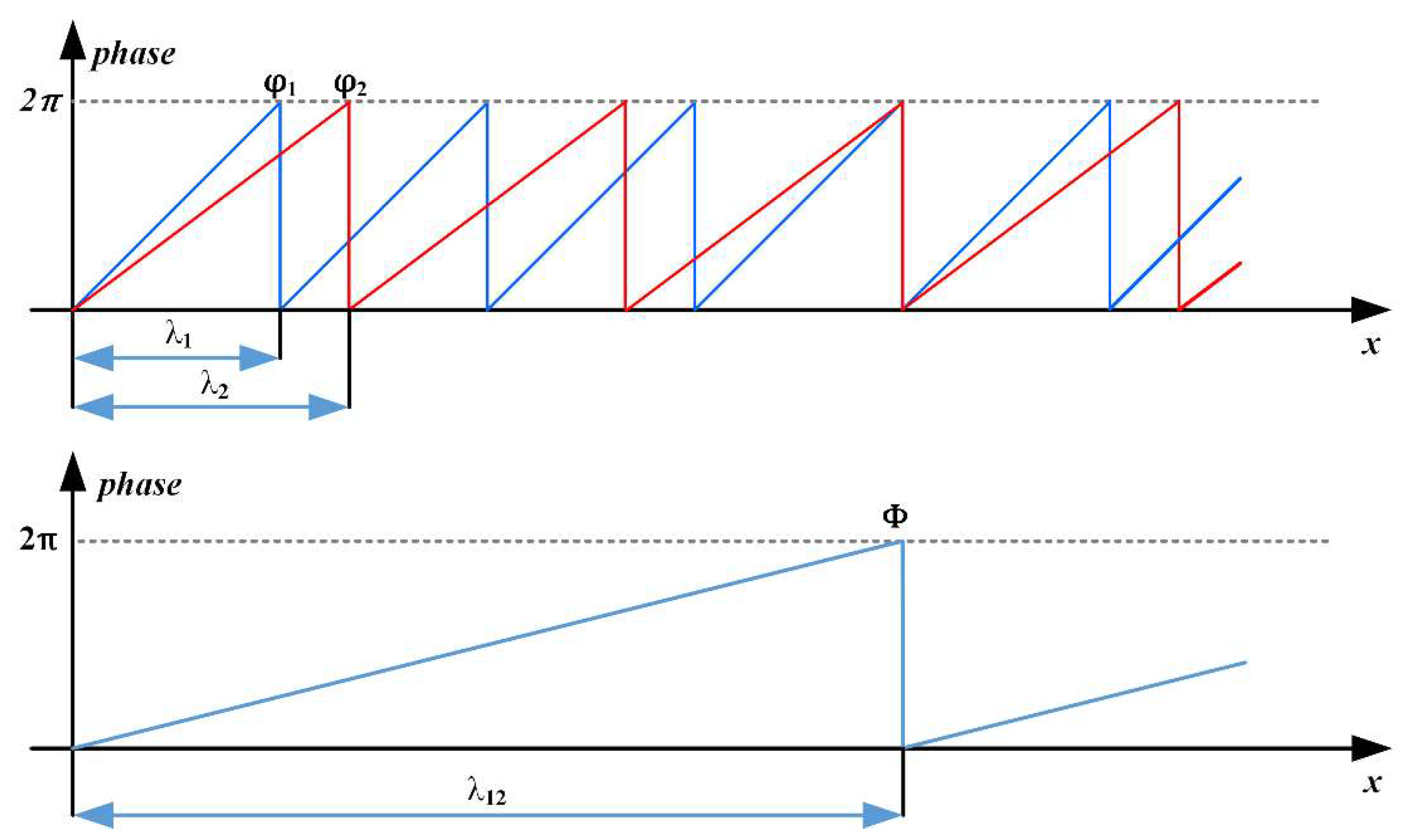
Figure 1, the frequencies of the phase functions
have to be chosen in a way that the resulting beat function
is unambiguous over the field of view. For the situation of
,
and
are corresponding wavelengths of
and
, respectively, and the heterodyne wavelength
can be solved according to the following equation:
If
and
are the unwrapped phases of
and
, respectively, it is easy to get:
From Equations (4) and (5), we have:
or
in which
is the rounding function. Therefore, we get a lower frequency
through
and
. Similarly, we can continue the multi-frequency heterodyne if we have more
until the final
has only one cycle in the entire field of view.
To do so, we can divide the multi-frequency phase-shifting method into two parts: the phase recovery and the multi-frequency heterodyne. Both depend on a pixel correspondence between the frames, which means that the same pixel coordinates in different frames from the same camera must represent the same point on the object. In the quiescent state, the frames are completely coincident in space, and the scenes contained therein are completely identical, but when a sequence is affected by a vibration, the coincidence between the frames is destroyed, and there is a certain degree of displacement between them.
In a multi-frequency, phase-shifting sequence of
m frequencies with
n phases for each frequency, the motion between the frequencies can be regarded as the motion between the
ith frame of one frequency and the
ith frame of the neighboring frequency. Likewise, the motion between phases can be regarded as the motion between a frame and its neighboring frame within the same frequency. It is easy to understand that the displacement between frequencies is
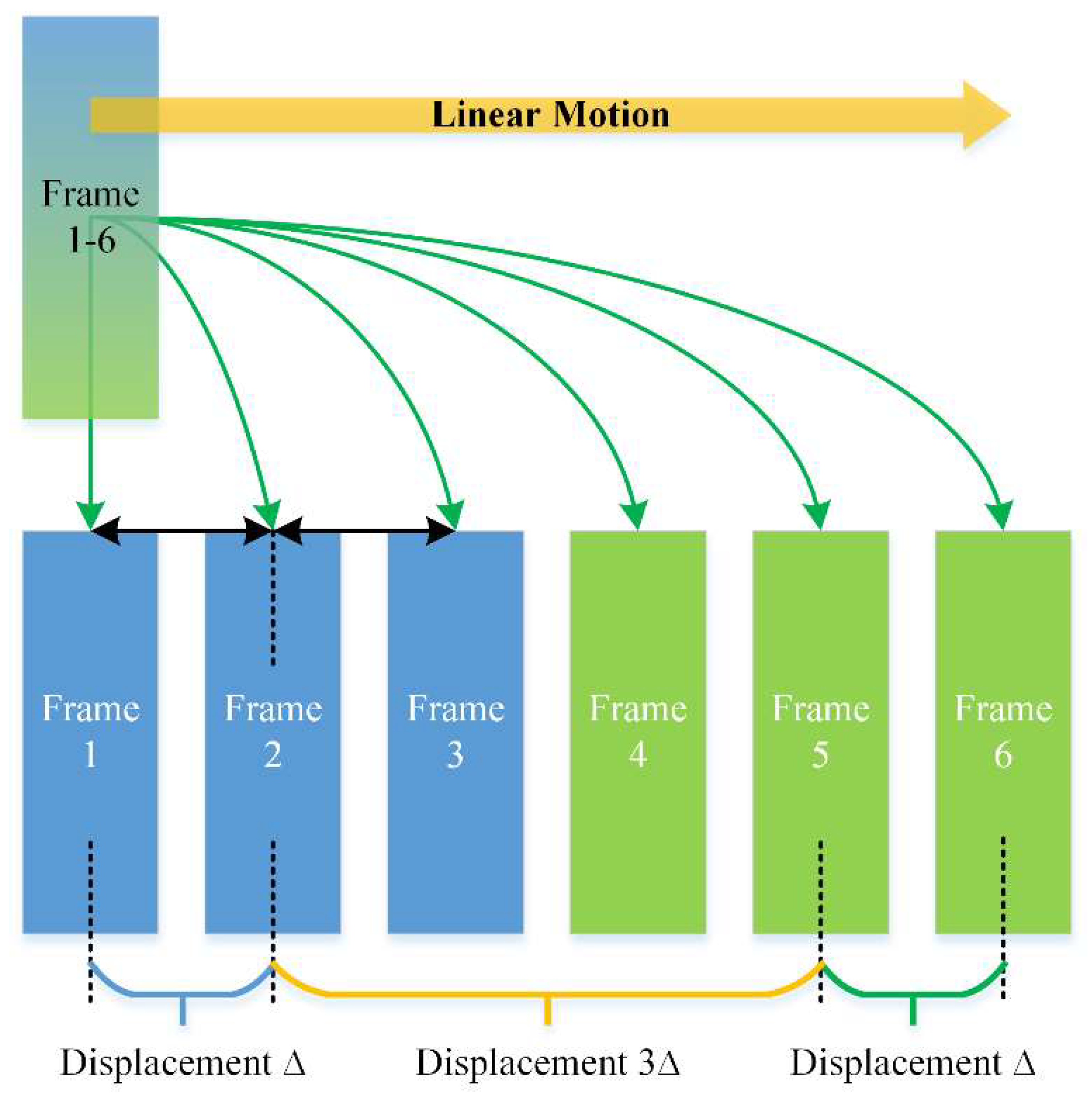
n times that between the phase-shifting frames. For example, in a two-frequency, three-step phase-shifting sequence affected by linear motion, there are six frames (
Figure 2). Frames 1–3 belong to the first frequency and frames 4–6 belong to the second. The displacement within a frequency is ∆. Consider the second frame as the reference, then the displacement between the two frequencies is 3∆, which is three times that of the three-step phase-shifting subsequence. Based on this analysis, it can be considered that the multi-frequency heterodyne process is more susceptible to vibration than the phase recovery process.
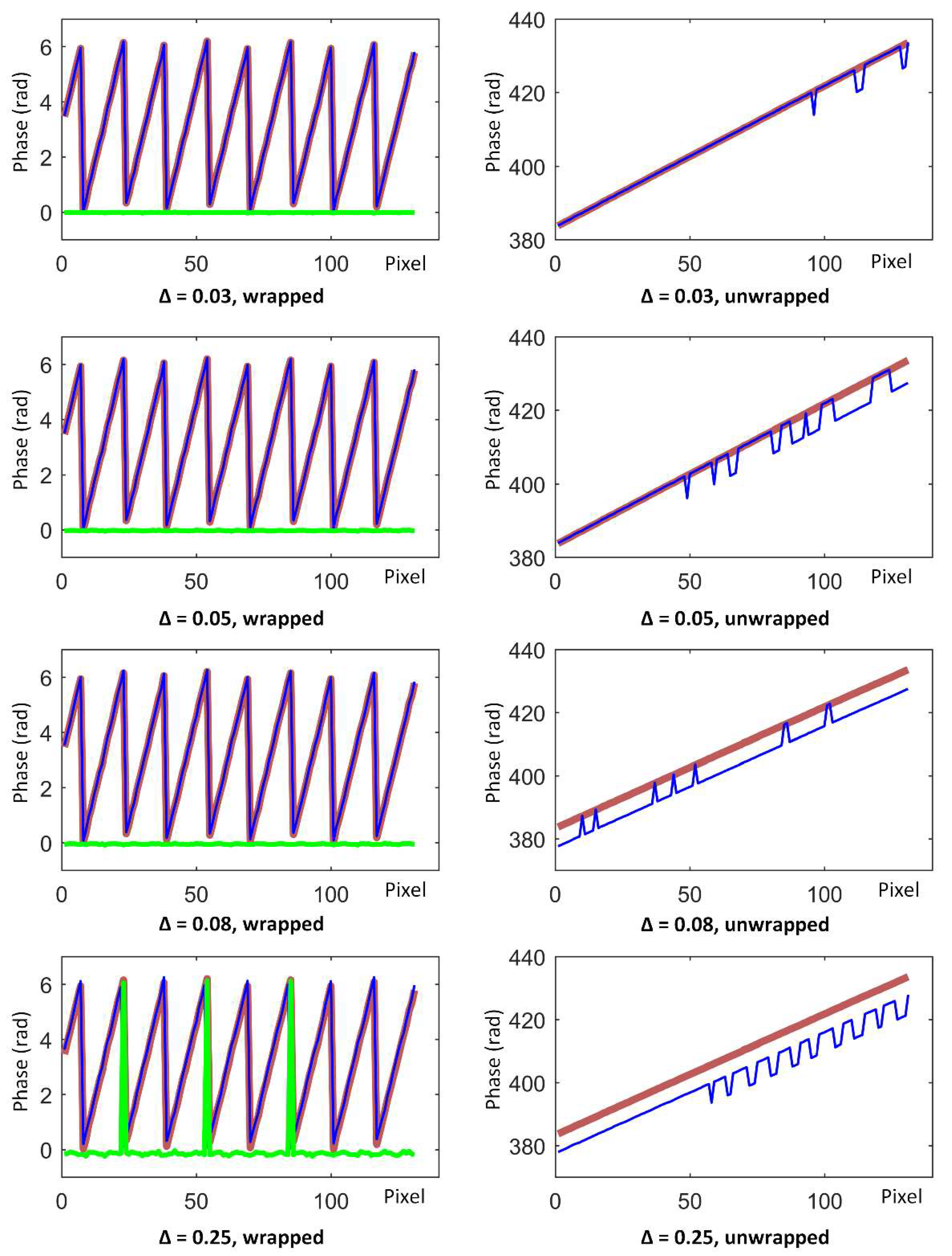
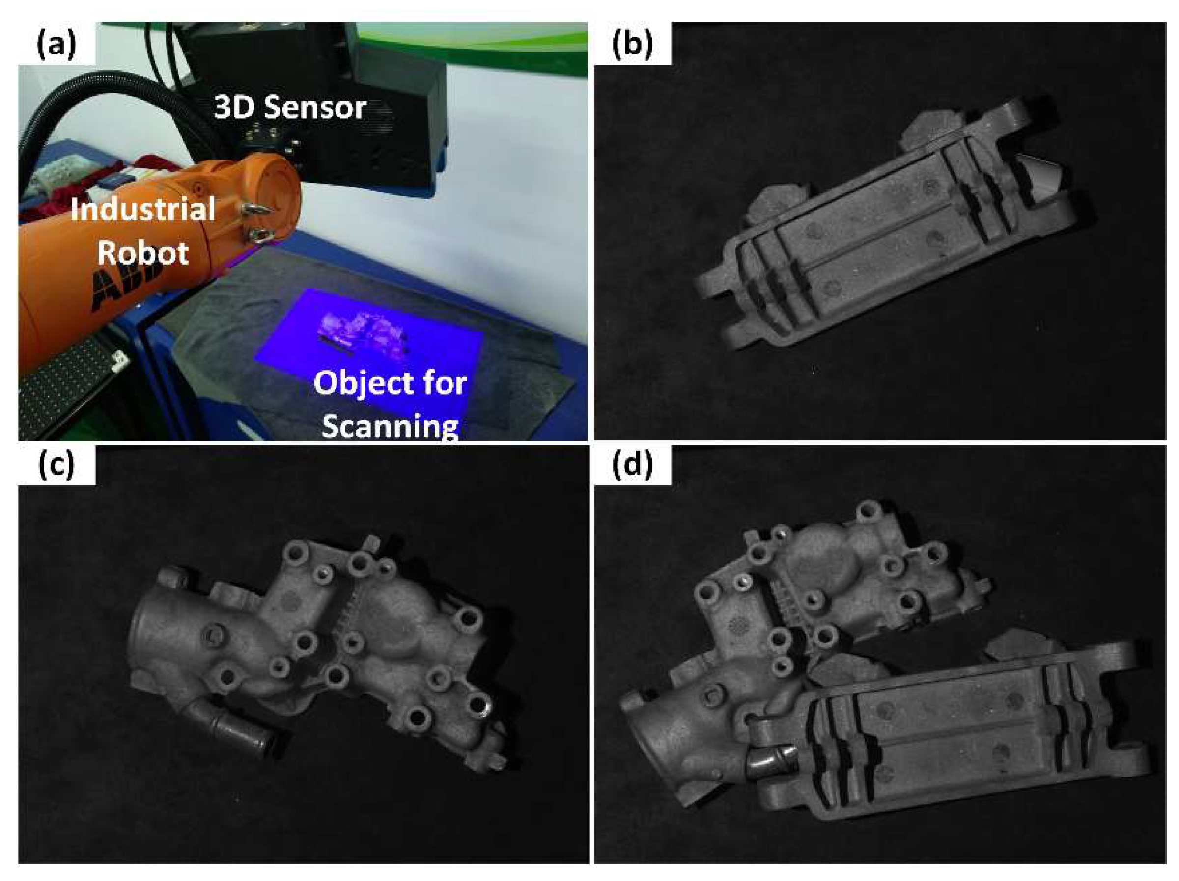
To quantitatively clarify this concept, we designed the following experiment: we considered a three-frequency, four-step phase-shifting image sequence of a piece of paper, where the purpose of selecting a piece of paper as a target was to obtain a relatively linear unwrapped phase for easy comparison. We project 12 images of a three-frequency, four-step phase-shifting sequence onto a flat white paper and captured them synchronously with the camera. We moved each image ∆ pixels to the right, relative to the previous frame in a direction perpendicular to the fringes, which means that the
ith image will move (
i − 1)∆ pixels from its origin.
Figure 3 shows the wrapped and unwrapped phases (obtained using the aforementioned methods) with different ∆s, before and after movement. The thick red lines are from the original sequence, the thin blue lines are from the moved sequence, and the green line is the phase error. In each graph, the abscissa is a pixel interval with a width of 140 pixels (unit: 1), and the ordinate is a phase value (unit: rad). From the experiment, we easily found that as ∆ rose from 0.03 to 0.08, the unwrapped phase error kept growing but the wrapped phase error was close to 0 and had no significant change. Until ∆ reached the considerable amount of 0.25, the wrapped phase error was easy to identify while the unwrapped phase error became more significant. This result means that in the process of gradually increasing the vibration intensity, the multi-frequency heterodyne process was affected first, when compared to the phase recovery process. In other words, below a certain vibration intensity, the phase-shifting subsequence was unaffected, but the constraints between multiple frequencies were destroyed, which is exactly the case of the relatively low frequency vibration discussed in this paper.
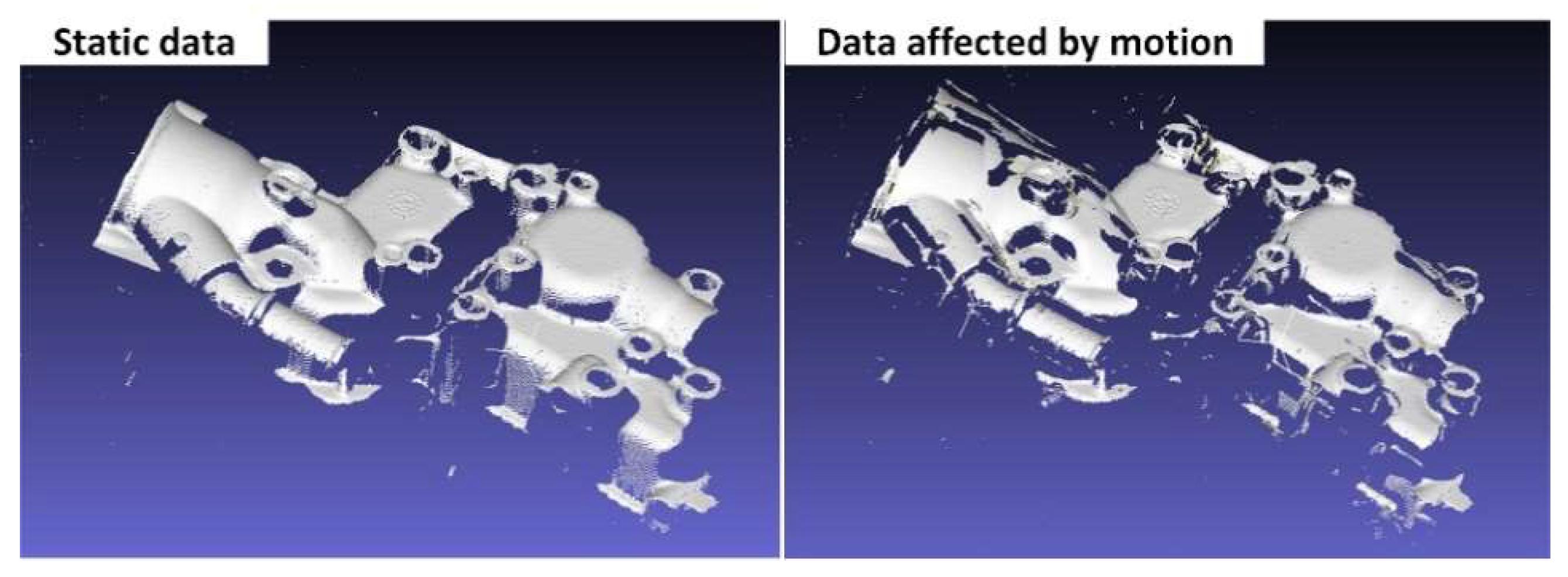
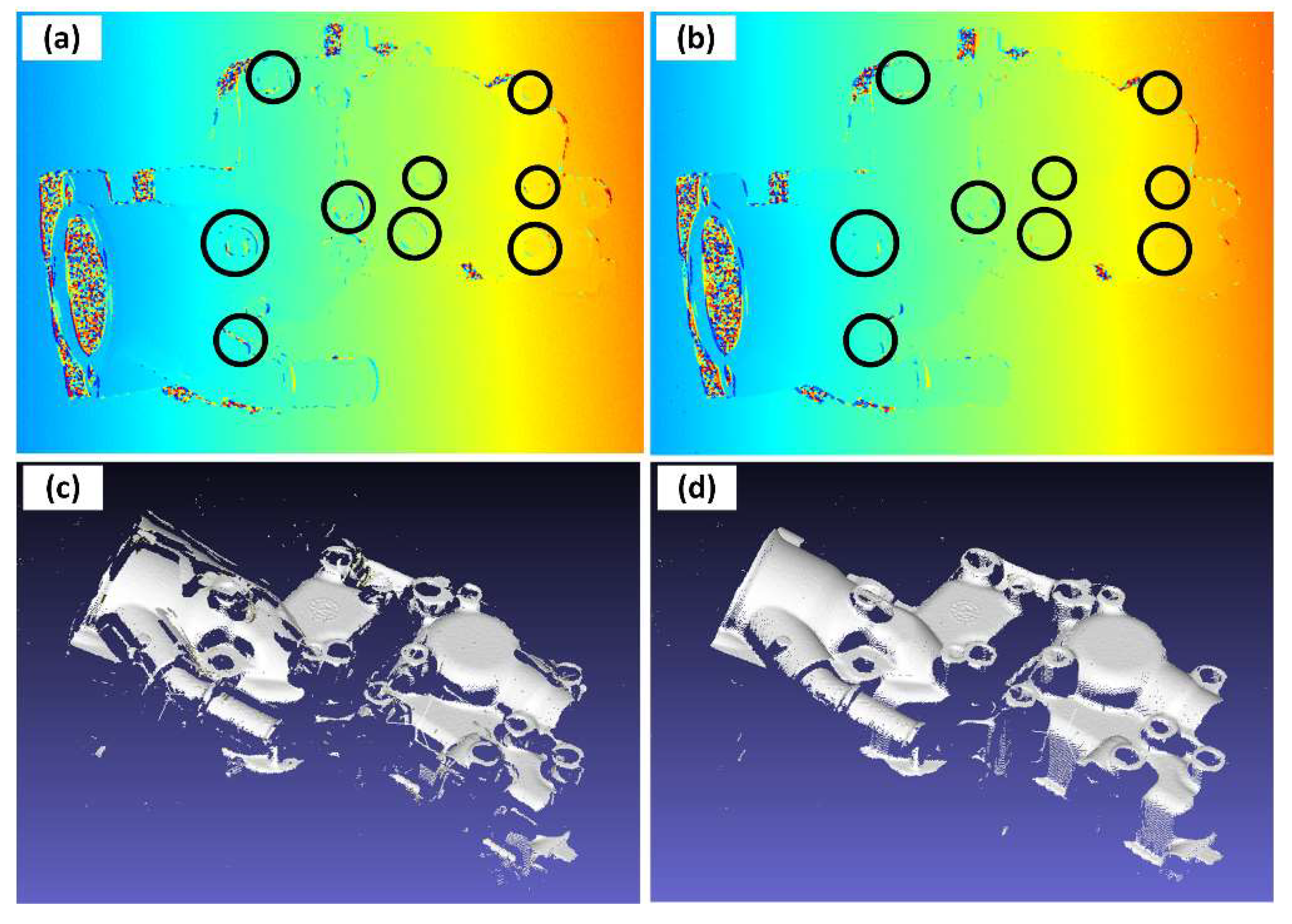
In the case of relatively low frequency vibrations, the motion error within the phase-shifting sequence of a certain frequency is small enough to be omitted or is easily removed using temporal phase-recovery algorithms, but the pixel correspondence between frequencies might be damaged. In these situations, there will be wrong phase unwrapping results and destroyed 3D reconstructions. As
Figure 4 shows, the 3D reconstruction from a multi-frequency, phase-shifting sequence in motion will have “broken” surfaces, which is the main form of motion error in a multi-frequency phase-shifting sequence. As seen in
Figure 3 when
and
, the 3D data affected by the vibration may be intact in the localized region, but have a “broken” surface globally. This is different from the vibration-affected phase-shifting subsequence, where there will be global ripples, outliers, etc.
2.2. Vibration Detection and Motion Compensation
In the multi-frequency phase-shifting method, the information is redundant if the ambient light image,
A, can be regarded as a constant [
16]. For the
N-step phase-shifting pattern sequence, knowing that
, we can easily obtain:
which means that the linear superposition of the fringe images will eliminate the streak component. If multiple reflections are ignored, the resulting image is no different than a uniformly illuminated image. In fact, in the measurement of non-high-reflecting objects, the superposition image is very close to the uniformly illuminated image; the absolute difference is almost negligible. In a multi-frequency phase-shifting sequence, the superposition of each frequency results in a uniformly illuminated image (which is known as a virtual frame) and the whole sequence can be fused as a series of uniformly illuminated virtual frames.
According to phase-shifting motion compensation studies, if the image sequence is affected by vibration or motion, an additional phase shift is introduced [
11]. Under these circumstances, the linear superposition will still have the streak component. With an additional phase shift
between frames and defining
and
, we have:
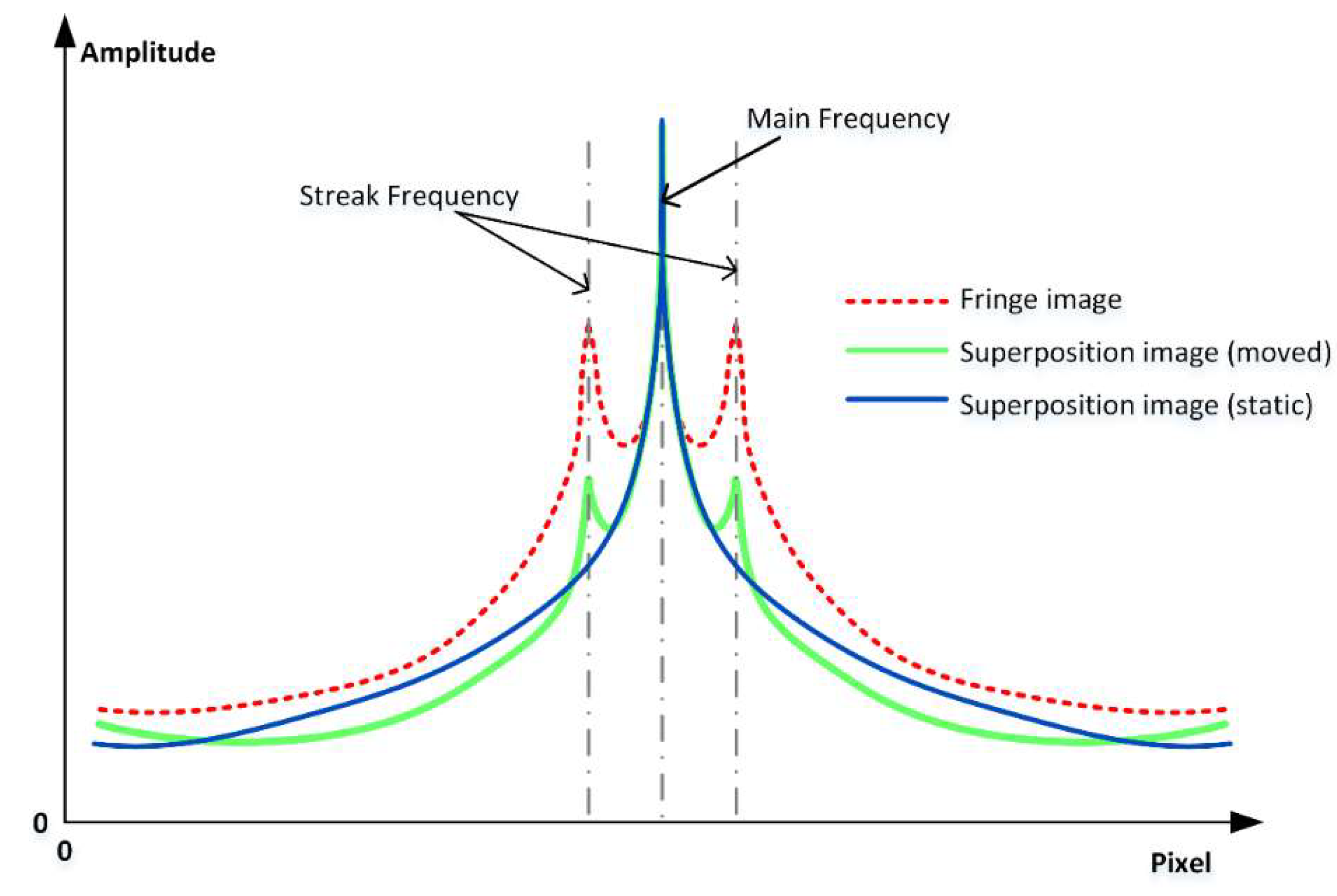
Obviously, the magnitude of the additional phase shift determines the strength of the streak component. In other words, the streak intensity indicates the magnitude of the vibration or motion. By extracting the ROI (region of interest) from the Fourier transform map of the fringe image and applying it to the superposition image, we can extract the peak of the streak frequency in the superposition image and compare it with the corresponding peak in the fringe image, as
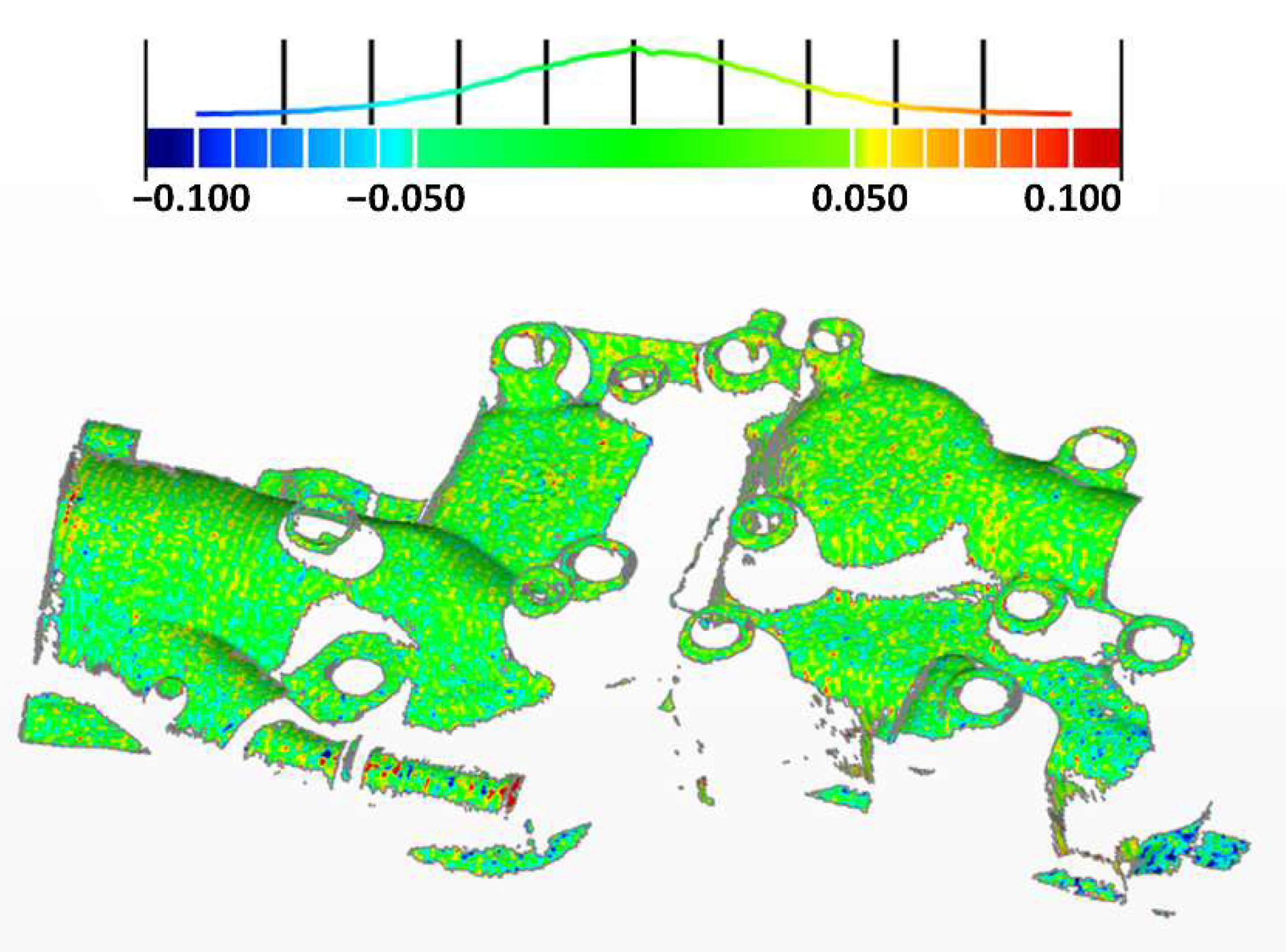
Figure 4 shows. It should be noted that
Figure 5 is only a schematic diagram drawn according to the Fourier transform maps, and the data in the graph is not strictly accurate. There will be visible streaks if the vibration or motion is strong enough, but in relatively low frequency vibration situations, the additional phase shift
may be too small for detection. In these situations, another criterion is proposed to quantitatively evaluate the motion intensity.
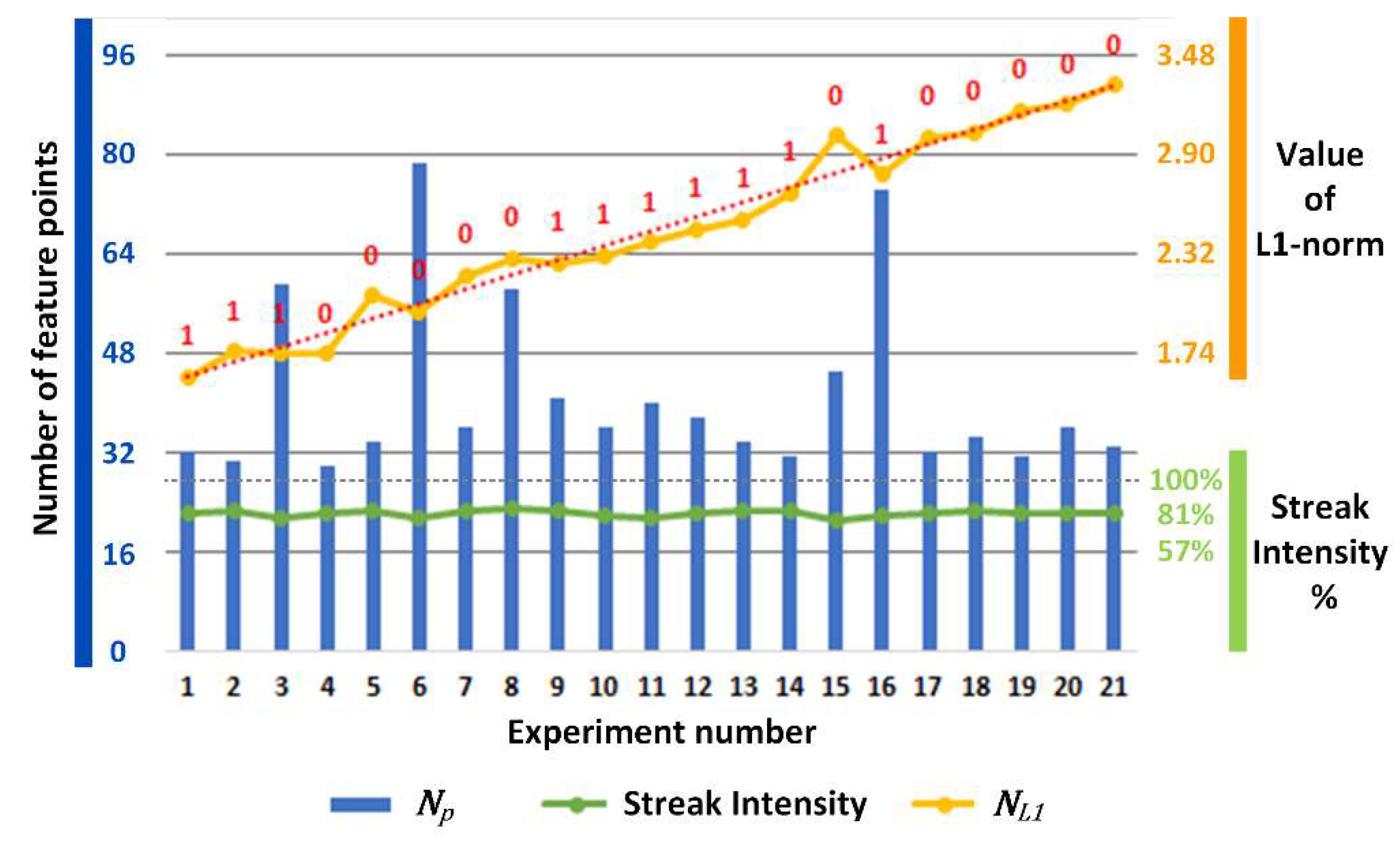
If the streak intensity is lower than a certain threshold, the streak component of the virtual frame can be omitted, and the grayscale feature point detection can be applied to the virtual frame. As mentioned in
Section 2.1, in a motion or vibration situation, the same point on the object will have different pixel coordinates in neighboring frames. The difference between the feature point arrays of a virtual frame pair indicates the motion intensity between the two virtual frames. The L1-norm can be used as an indicator for this difference, which is positively correlated with vibration intensity. Supposing that
represents the feature point array in the first virtual frame and
in the second, and
represents the number of points in
(which is also the number of points in
), we have a metric
for the relative movement between the virtual frames:
Furthermore, a homography matrix can be calculated from
and
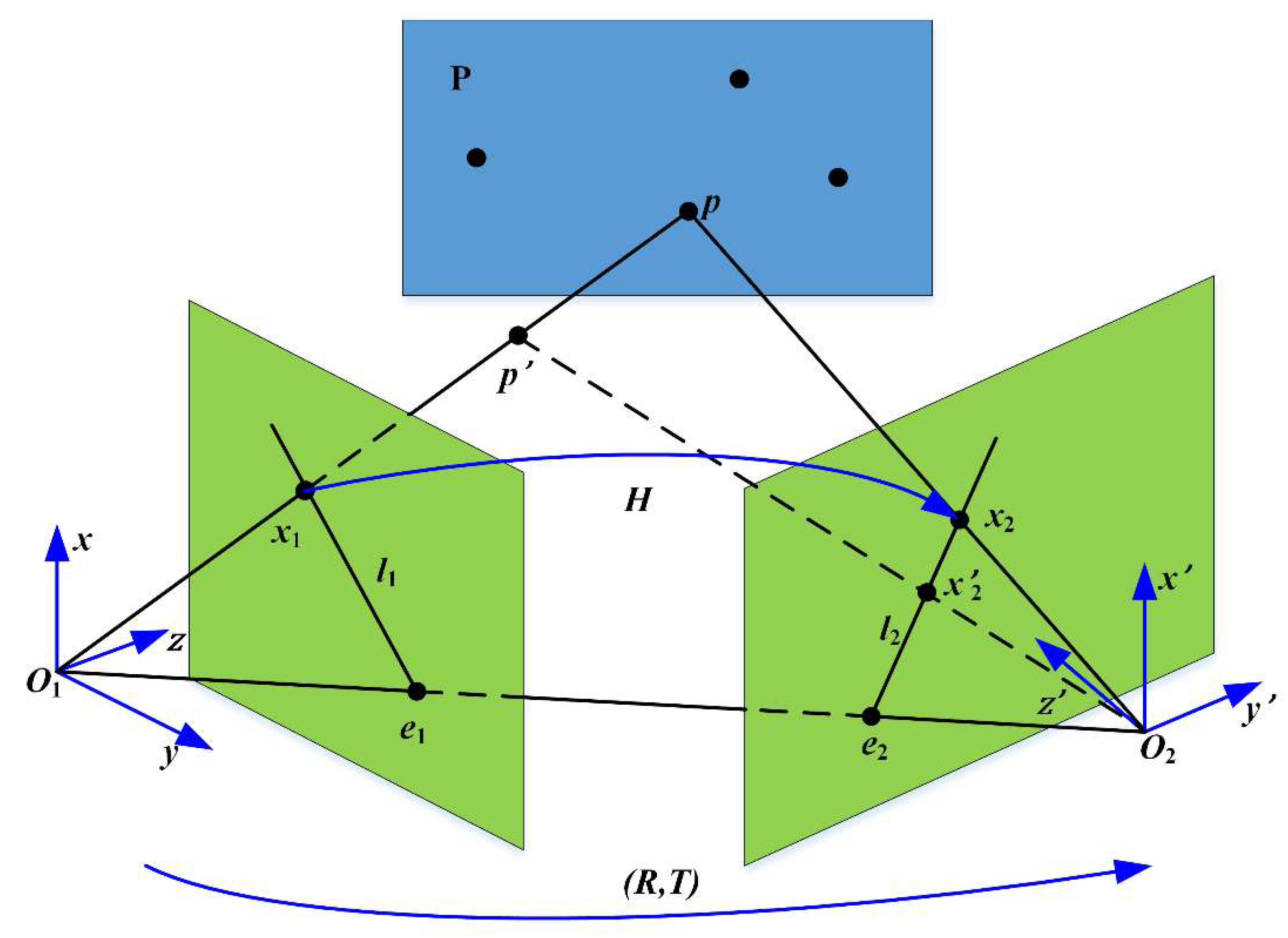
. The homography matrix is usually used to describe the transformation between images when there is the same plane in two images. There is relative motion between the target and a camera in vibration. If we think the target position is the same, then the camera’s pose is different in two consecutive frames. For points out of plane, homography may not be appropriate for images taken in two camera poses. As
Figure 6 shows, in the camera coordinate system
and
of two poses,
and
are the image points of
, which is a point out of plane
, and
is the mapped point of
using homography
. It is easily found that for a point
, the difference between
and
represents the error of homography. Additionally, we define the following:
is the baseline between two camera poses,
and
are the epipoles, and
and
are the epipolar lines. The difference between
and
is called the parallax. It should be noted that in the illustration herein, the two coordinate systems
and
represent different poses of the same camera, rather than two cameras in stereo vision, whose parallax far exceeds the description range of the homography matrix.
It is easy to prove that
depends on
and the norm of
(or length of
because
). If the parallax between two images is low enough or there is only rotation of the camera pose between two images, in other words the translation
between
and
is small enough relative to the scene depth
, the homography matrix will be accurate enough to describe the correspondence of all points in two images even when they are not on the same plane [
17]. If the vibration-caused camera motion is small enough relative to the scene depth, the parallax between the two virtual frames is low and the homography matrix is sufficiently accurate for global pixel mapping. For virtual frame sequences that pass the frequency check, the corresponding feature points of the virtual frames can be extracted, and then the homography mapping between two virtual frames can be found.
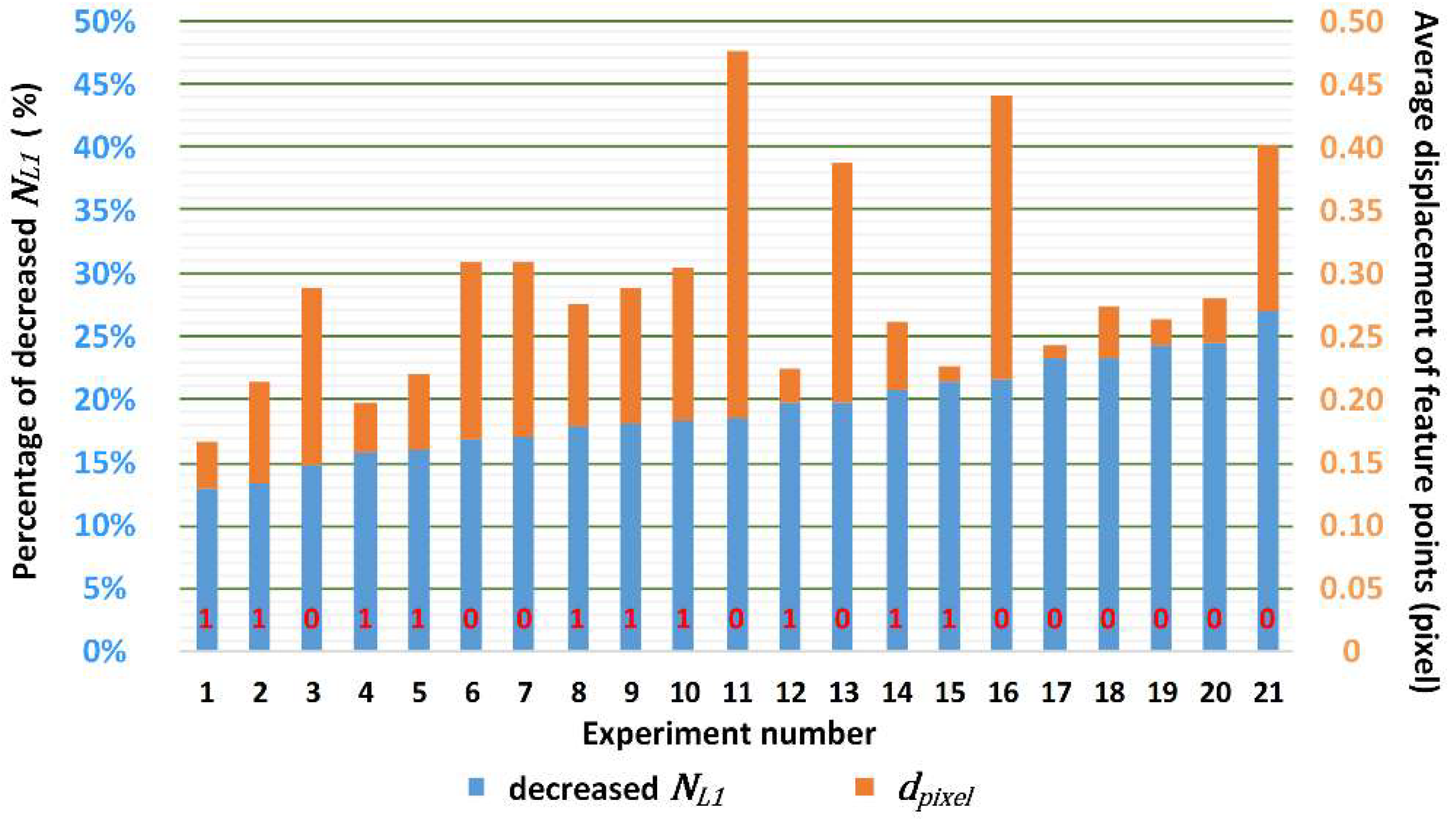
Furthermore, as long as there are more than eight non-coplanar feature points in a pair, the accuracy of this correspondence can be evaluated by calculating
again after the corresponding points have been mapped by the homography matrix. In this sense, the method itself limits its scope of use, and excessive vibration or motion of the camera will be discovered during repeated L1-norm calculations to avoid meaningless or mistaken compensation. When the homography matrix is used to map one image to another, there is interpolation and pixel rounding in the process as digital images have integer pixel coordinates and gray values while feature points have sub-pixel level coordinates. By considering this, we introduced the average pixel displacement
to indicate the consistency of feature points after the virtual frame was mapped by the homography matrix. This can be expressed as:
supposing that
,
, and
is the order of feature points, we have
and
, which means that
depends on the Euclidean distance between each pair of feature points, and
depends on the Euclidean distance between the mean values of all feature points in two arrays.
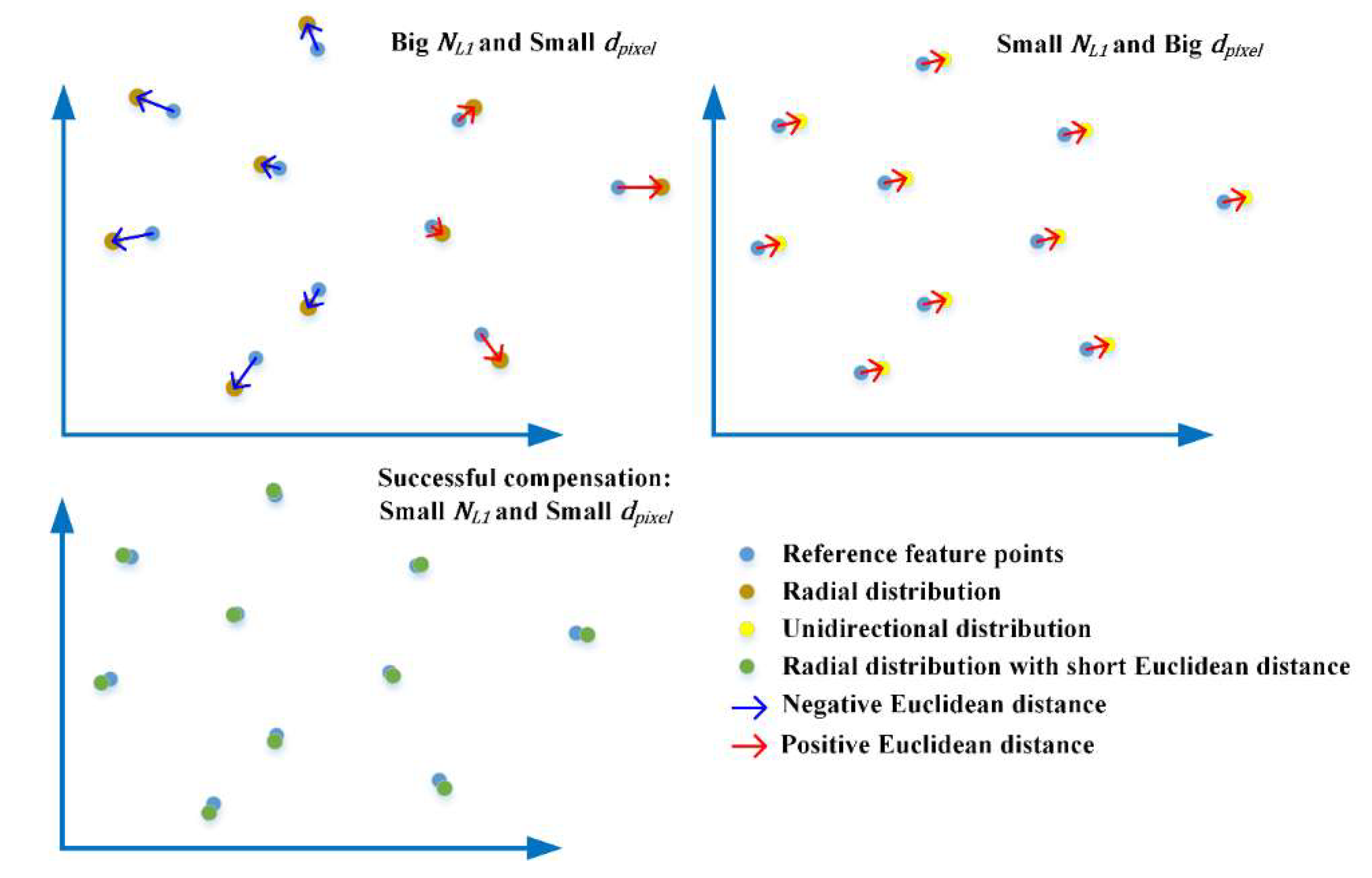
The difference between
and
is that
indicates the absolute difference between two point arrays, which is non-directional, but
is directional, as shown in
Figure 7. This means that if a point array is evenly radially distributed relative to another point array, it will have a small
while the
is big. Conversely, if one set of points is unidirectionally distributed relative to the other, the
may be big even when the
is small. The introduction of
is to indicate the situation where after compensation,
decreases but the compensated virtual frame still has a unidirectional displacement to the reference virtual frame. According to the experiment in
Section 2.1, the unidirectional displacement is critical to phase unwrapping.
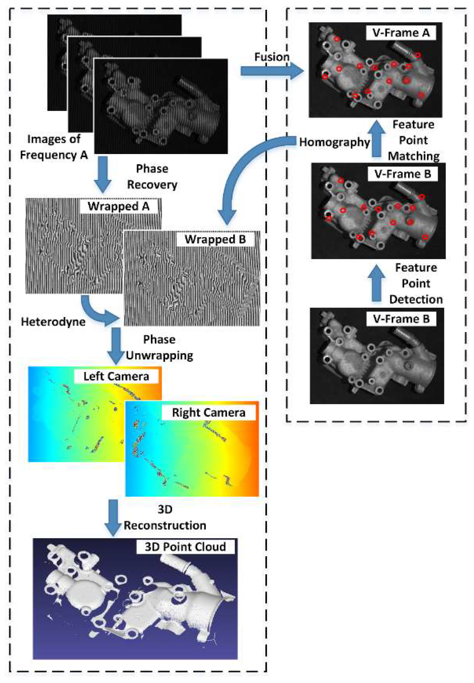
In the multi-frequency, phase-shifting fringe projection methods, the wrapped phase is calculated using the images of the same frequency and the unwrapped phase is obtained using the heterodyne from different wrapped phase images [
9]. From above, we know that the homography matrix can be used to map two images affected by vibration in a low parallax situation. If it is suitable for the homography matrix to map the virtual frames superimposed from the phase-shifting subsequence, it can also be applied to the wrapped phase maps. The heterodyne algorithm recovers the absolute phase information based on the phase values of the same pixel in different wrapped phase maps. Noises and errors of the unwrapped phase come from the destruction of the pixel correspondence. As the homography matrix obtained from the feature points is sufficiently accurate for the global pixel mapping in the vibration situation, it can be applied to correct the pixel correspondence between the wrapped phase maps. The operation flow is shown in
Figure 8. For the sake of simplicity, we used the reconstruction process of a two-frequency, three-step phase-shifting as an example. Among the six images captured by the left camera, the three images belonging to the same frequency A can generate a wrapped phase map, Wrapped A. In our method, they can simultaneously synthesize a virtual frame, V-Frame A. Similarly, there are the Wrapped B and V-Frame B. Due to the influence of vibration, the pixel correspondence between Wrapped A and Wrapped B was destroyed. In our method, the SIFT (scale-invariant feature transform) method was used to detect feature points in V-Frame A and V-Frame B. The reason for choosing the SIFT method is that it is invariant in perspective transformation and is not sensitive to grayscale changes. Then two arrays of feature points were matched by the FLANN (fast library for approximate nearest neighbor) matcher and according to the average Euclidean distance, the mismatched pairs with excessive distance were screened out. Then, we obtained a homography matrix from two arrays of feature points that mapped V-Frame B to V-Frame A. We then applied the same homography matrix used to map Wrapped B to Wrapped A. Therefore, the pixel correspondence between them was corrected. Using the Wrapped A and corrected Wrapped B, we could obtain the unwrapped phase map of the left camera, where the same thing happens on the right camera. In the end, the correct 3D reconstruction results were generated.

 ,
, 


