Abstract
This manuscript describes the Microwave Interferometric Reflectometer (MIR) instrument, a multi-beam dual-band GNSS-Reflectometer with beam-steering capabilities built to assess the performance of a PAssive Reflectrometry and Interferometry System—In Orbit Demonstrator (PARIS-IoD) like instrument and to compare the performance of different GNSS-R techniques and signals. The instrument is capable of tracking up to 4 different GNSS satellites, two at L1/E1 band, and two at L5/E5 band. The calibration procedure of the up- and down-looking arrays is presented, the calibration performance is evaluated, and the results of the validation experiments carried out before the field experiments are shown in this paper.
Keywords:
GNSS; Reflectometry; remote sensing; antenna array; beamforming; beam steering; calibration 1. Introduction
When Global Navigation Satellite Systems—Reflectometry (GNSS-R) was first proposed in 1988 for multistatic scatterometric applications [1], the Global Positioning System (GPS) was the only one available and with a limited number of broadcasted signals. At that time, the only publicly available signal was the L1 C/A, which has a narrow bandwidth (2 MHz), and therefore limited ranging accuracy, while the private signals such as the precise code P(Y), and the military signal M have a wider spectrum (≈20–30 MHz). In order to take advantage of the wide spectrum signals, the so called interferometric technique (iGNSS-R) was proposed in 1993 [2]. It consists of the correlation between the reflected signals on the Earth’s surface and the signal received directly from the same transmitting satellite. In this way, it is not necessary to know the transmitted codes, and it is possible to take advantage of the wider signals. However, since both signals are received with a poor Signal-to-Noise Ratio (SNR), high directive antennas are needed. Besides, the correlation of the two received signals is sensitive to be affected by Radio Frequency Interference (RFI) [3], and by satellite cross-talk [4]. Later on, the nowadays called conventional technique (cGNSS-R) was proposed in 1996 [5]. It consists on the cross-correlation between the reflected signals with a locally generated clean replica of the transmitted code. In this way, the achieved SNR is higher and the effect of other satellites and RFI is mitigated, but only the narrow-band open signals can be used.
Nowadays, more GNSS systems have been deployed and wider signals are being broadcasted, such as the public Galileo E5 signal, with more than 40 MHz bandwidth [6]. While a performance comparison of these signals has been studied with simulated data [7], they have never been compared with real data in similar conditions. For this reason, during the past years a new airborne instrument has been developed at Universitat Politècnica de Catalunya: the Microwave Interferometric Reflectometer (MIR).
This manuscript describes the MIR instrument, the calibration procedure, and shows the validation results of the experiments that were conducted to prove its performance.
2. Instrument Overview
The MIR instrument is a GNSS reflectometer that has two steerable arrays. The up-looking one points directly to the GNSS satellites, while the down-looking one points where the signals from these satellites are reflected on the Earth’s surface. Each of these arrays is connected to an analog beamformer that creates two beams at L1/E1 (1575.42 MHz) and two beams at L5/E5a (1176.45 MHz), therefore the instrument can track up to 4 different satellites, and their corresponding specular reflection points. The signals received from a satellite by the up-looking array are sampled synchronously by pairs with the signal from the same satellite received by the down-looking array after reflecting on the Earth’s surface. The signals coming from the down-looking array are amplified prior to be sampled in order to compensate the losses caused by scattering from various landscapes, including rough and vegetated ground. The data is sampled using SDRs and then is stored for post-processing. The instrument is controlled by a Linux embedded computer that selects the best available satellites and points the instrument beams towards them, and to the expected specular reflection points taking into account the position of the satellites and the position and attitude of the plane. Last, the instrument has a calibration system that generates PseudoRandom Noise (PRN) codes to calibrate the instrument in amplitude and phase. Figure 1 shows the instrument block diagram. The next subsections explain all blocks in detail.
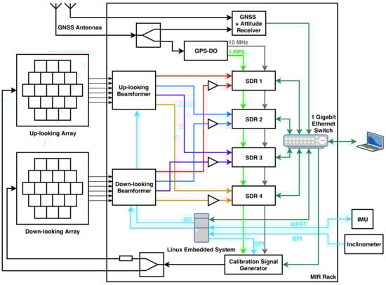
Figure 1.
Block diagram of the MIR instrument. The red, blue, orange, and purple lines correspond to the radio frequency (RF) signals of each of the four beams from both the up- and the down-looking array. The light green is a 1 Pulse Per Second (PPS) signal. The grey line is a 10 MHz reference signal. The cyan lines correspond to serial protocols of communication, such as Inter-Integrated Circuit (I2C), Serial Peripheral Interface (SPI) or Universal Asynchronous Receiver-Transmitter (UART). The dark green lines are Ethernet lines. The black lines are other radio frequency (RF) signals, such as the calibration signals, or the GNSS signals for the GNSS receiver. SDR stands for Software Defined Radio. IMU stands for Inertial Measurement Unit. GPS-DO stands for GPS—Disciplined Oscillator.
2.1. Antenna Array and RF Front-Ends
MIR has two antenna arrays, an up-looking Right Hand Circular Polarized (RHCP), and a down-looking Left Hand Circular Polarized (LHCP) one. Each array has 19 dual-band patch antennas. The antenna elements are dual-band patch antennas of about 95 * 95 * 8 mm specifically designed for the instrument [8]. The antennas (Figure 2) are made of two square patches stacked between dielectric substrates (Rogers 4003c) that resonate at the L1/E1 central frequency (1575.42 GHz), and at the E5 central frequency (1191.795 GHz), respectively. The antenna is fed by capacitive coupling using a cross-shaped patch on the top of the antenna, which is itself electrically fed by two probes. The cross-shape of the feeding patch was found to be useful to increase the bandwidth of the antenna, but at the expense of reducing the axial ratio of the antenna [8]. A thick dielectric layer between the L5 patch and the ground plane was used to increase the bandwidth. The feeding patch dimensions and the position of the feeding coaxial cables/connectors along the antenna axes were optimized to maximize the bandwidth and the matching of the antenna at the aforementioned frequency bands.
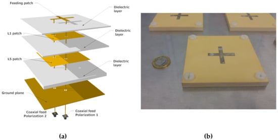
Figure 2.
3D model of the antenna elements (a), and photography of one of the manufactured antennas (b). The antenna measures 95 × 95 × 8 mm.
Four manufactured elements were measured and they showed an average bandwidth at −10 dB of ≈20 MHz at L1/E1, and ≈34 MHz at L5/E5a. The antenna radiation pattern of one of the antenna elements at the different frequency bands was measured at both frequency bands (Figure 3) in the Universitat Politècnica de Catalunya (UPC) AntennaLab anechoic chamber, and also the cross-polarization pattern (see Figure 4). The antenna directivities in each band are shown in Table 1. The efficiency was measured using calibrated reference antennas.
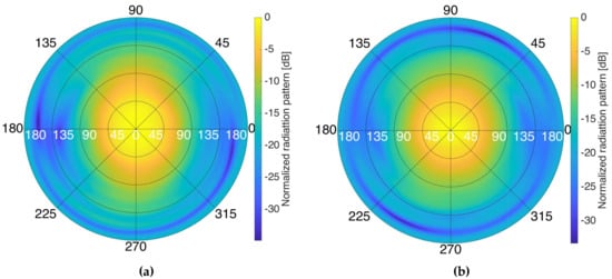
Figure 3.
Measured antenna radiation pattern of one of the manufactured antennas at L1/E1 (a), and at L5/E5 (b).
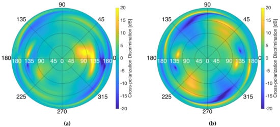
Figure 4.
Measured cross-polarization discrimination patterns at L1/E1 (a), and L5/E5a (b) frequency bands. The colorscale was limited to ±20 dB to ease the viewing.

Table 1.
Measured directivity and estimated efficiency of the antenna elements.
The antennas are separated 0.75 and 0.56 over a regular hexagonal grid. The down-looking array is mounted in a squared ground plane of 860 mm per side that weights 25 kg approximately, and the up-looking one in a ground plane of 800 mm per side that weights 18 kg approximately (Figure 5). The arrays have a 19-ports power splitter attached to the structure. These devices split the calibration signal and inject the resulting signals to each Radio Frequency (RF) Front-end. The directivity of both arrays was measured in the anechoic chamber as explained later in Section 4.1 and is shown in Table 2.
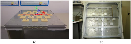
Figure 5.
Top view of the up-looking array (a), and back view (uncovered) of the down-looking array (b). The up-looking array image includes the baseline used to define each antenna element by a pair of values. The azimuthal pointing angle is defined anti-clockwise from vector to . The off-boresight pointing angle is defined from vector to the antenna array ground plane.
Table 2.
Measured directivity of the arrays.
The RF Front-ends are attached directly behind the antennas. A 90 hybrid combines the two linear polarizations to generate a circular polarization: RHCP for the zenith looking antenna, and LHCP for the nadir looking one. The outgoing signal is then connected to one of the inputs of an RF switch. The other input is used to inject a calibration signal. The switch is always commuted to the antenna signal, behaving thus as a directional coupler. The combined signals are amplified with a Low Noise Amplifier (LNA) (G ≈ 15 dB, NF ≈ 0.8 dB), high-pass filtered ( MHz) to attenuate broadcasted Frequency Modulation (FM) signals (80–100 MHz) and Global System for Mobile communications (GSM) signals (800–900 MHz), amplified again (G ≈ 22 dB, NF ≈ 2.1 dB), and low-pass filtered ( MHz) to attenuate broadcasted GSM signals (1700–1900 MHz) and Wi-Fi signals (2.4 GHz), and to avoid undesired high-frequency oscillations. Wi-Fi signals might not affect during flight operations, but are filtered to avoid any interference in laboratory tests.
2.2. Beamformer
Since digital beamforming would require an enormous amount of resources to be implemented (2 bands × 2 arrays × 19 antennas = 76 data streams to be sampled simultaneously and stored), two analog beamformers were implemented. Each beamformer block (Figure 6) consists of 19 boards that generate 4 different analog steerable beams for each array. Each board is connected to an RF Front-end. First, it divides the incoming signal into two branches, then they are amplified (G = 17 dB), and then they are band-pass filtered at the L1, or the L5 bands using Surface Acoustic Wave (SAW) filters. The L1 filter is centered at 1583 MHz, and has a bandwidth at −3 dB of 58 MHz. The L5 filter is centered at 1178.12 MHz and has a bandwidth at −3 dB of 55 MHz. Each of these branches is split again to generate two different beams for each band. The amplitude and phase of these signals is then modified to steer the beams electronically to the desired direction. Last, the 19 signals of each beam are combined with a 19-port power combiner, obtaining thus 4 RF lines, one for each particular band and beam. There is one of these beamformer blocks for each array.
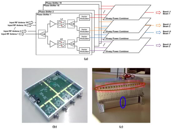
Figure 6.
Block diagram of one of the beamformers (a), close view of one of the phase shifters manufactured (b), and front picture of one of the assembled beamformers (c). Note in the assembled beamformer 19 inputs (red), and the 4 outputs (blue).
After the scattering on the Earth’s surface, the reflected signal power in an airborne case is expected to be 0–30 dB lower than the direct one [9]. In order to compensate this expected power loss, two RF amplifiers with a total gain of ≈35 dB were placed after the beamformer.
The beam-forming was implemented with ADL5390 Vector Modulators [10], which are used as variable amplifiers and phase shifters. This device (Figure 7) amplifies or attenuates individually the I and Q components of the signal according to the voltage applied to the gain control pins. In this way, the magnitude and phase of the input is changed. Without any unbalance introduced by the vector modulator or the hybrid coupler, the vector modulator and the later combiner, the output signal is
where I and Q are the voltage gains in the I and Q channels, respectively (note that they can be negative), is the input signal, is the output signal, g and are the gain and phase in the whole RF chain (the phase in the Q branch is radians larger), is the carrier angular frequency, and is the 2-argument arctangent function.
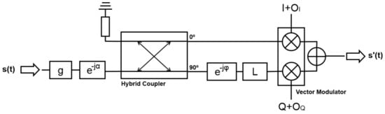
Figure 7.
Used model for a whole RF chain.
If the unbalances are taken into account, the output signal in the frequency domain becomes
where L and are the amplitude and phase unbalance introduced by the hybrid coupler, the vector modulator, and the power combiner, and and are the gain offsets in the I and Q channels, respectively. To simplify, the I and Q gains and the gain offsets will be written in vector notation as
Then, (2) becomes
The achieved gain can be represented in the I-Q plane (Figure 8). Ideally, if the values are swept, the achieved gain will be represented as a constant radius circle, centered at the origin, starting at over the I axis, and and will be orthogonal (blue vectors). Without calibrating, the circle will not be centered (due to the gain offset O), the circle will become an ellipsoid (due to the gain unbalance L), the gain vectors will not be orthogonal (due to the phase unbalance , see red vectors), and will be rotated around the plane origin (due to the phase ). Besides, if we plot the gain circles of all 19 vector modulators of a same beam, they will have different radii (due to different gains g in each RF chain). This effects will induce an error in the gain and phase set to any signal.
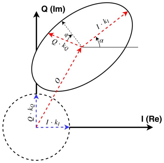
Figure 8.
Ideal gain circle (dashed line), and modeled gain ellipsoid (solid line) in the IQ gain plane.
2.3. Beam-Steering Control
The pins of the vector modulators that control the gain of the I and Q channels require a differential voltage, which is generated using 16-bits differential Digital-to-Analog Converters (DAC). These DACs are controlled using the Inter-Integrated Circuit (I2C) serial protocol and I2C multiplexers, which are controlled by the Linux embedded main controller.
The required I and Q gains are computed in near real time with an embedded system [11]. The system first retrieves the available satellites using the Trimble BD982 GNSS Receiver [12] and selects the two optimum available in each frequency band. This GNSS receiver is capable of tracking GPS, GLObalnaya NAvigatsionnaya Sputnikovaya Sistema (GLONASS), Galileo, and Satellite-Based Augmentation Systems (SBAS) in L1/E1, L2, and L5/E5 frequency bands. The satellites are chosen at each frequency band separately following the algorithm described in Figure 9. The system only takes into account satellites whose phase has been locked by the GNSS receiver. In this way, the GNSS receiver provides accurate Doppler frequency, that makes easier the post-processing. It prioritizes to pick one Galileo and one GPS satellites with the highest elevation angle if both elevation angles are over 65. If these conditions are not fulfilled, the system picks the two satellites with the highest elevation angles. The validation of the algorithm was conducted in the laboratory rooftop and the results are shown in Section 4.2.
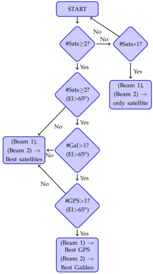
Figure 9.
Developed selection algorithm to choose the best satellites available [13].
In order to find where each array has to point, the system first estimates the position of the satellites in ECEF coordinates using the satellite ephemeris [6,14]. Then, the Earth Centered Earth Fixed coordinates (ECEF) of the satellites are transformed to the North-East-Down (NED) local coordinate system, where the satellites are located in the sky with an azimuth and an elevation angle. For the down-looking array, the location on ground to point is determined using a flat Earth model. Once the position of the satellites is known in a local reference plane, the vectors that point to them are rotated using Direction Cosine Matrices (DCM) taking into account both the orientation of the plane and the orientation of the arrays, so the vectors pointing to the satellites are now referenced in a local vehicle-carried coordinate system. If there are enough GNSS satellites in view, the orientation is estimated by the GNSS receiver, which has two antenna input connectors that can be used to determine two Euler angles, and an inclinometer [15], which gives the third rotation angle. If not, a Commercial Off-The-Shelf (COTS) Inertial Measurement Unit [16] is used. Then, the system computes the required I and Q gains for each vector modulator taking into account the position of the satellites, the position and the orientation of the platform, and the calibration parameters. The system also logs the platform position and attitude, the estimated position error, which satellites are pointed, their approximated Doppler frequency and the pointing angle of each array in the local reference system to later compensate the antenna radiation pattern. The ideal phase of each element is computed as
where d is the distance between antennas, is the wavelength at the particular frequency band, m and n are the coordinates of each antenna in the hexagonal grid defined in Figure 5, is the angle between the and vectors in Figure 5, is the azimuthal pointing angle defined anti-clockwise from vector to , and is the off-boresight pointing angle defined from vector to the antenna array ground plane.
Then, if a gain G and phase must be set to a particular branch, first the non-corrected and are found taking into account the gain g and phase of that particular RF branch:
Then, the L and parameters are compensated, and the corrected and are obtained:
The calibration parameters g, , L, and are obtained following the procedure described in Section 3.1. If any offset in the I or Q components and has to be compensated, it has to be removed from and . These two corrected gains are then written to the DACs using I2C protocol.
2.4. Data Sampling and Processing
For the data sampling, 4 dual-input Software Defined Radios (SDR) model Ettus Research Universal Software Radio Peripheral (USRP) X310 are used [17]. Each one samples synchronously a pair of beams. They are synchronized between them using a 1-PPS signal and a 10 MHz reference signal, both generated with an Octoclock [18] which uses for that purpose a GPS-Disciplined Oscillator (GPS-DO). The signals to be sampled are down-converted and sampled at 32.736 Msps and 1 bit for both the I and Q components of the signal, and then stored in a computer for post-processing.
2.5. Calibration System
The instrument calibration is conducted in two steps, the first one in an anechoic chamber, and the second one with a calibration system embedded in the instrument. This calibration system uses a periodic signal made of a concatenated sequence of 10 L5 PRN codes (10 × 10230 chips). The codes are generated in another SDR (URSP N210) at a 10 MHz chiprate (20 MHz bandwidth), with a total sequence length of 10 ms (the last 2300 chips are removed), and a repetition period of . The signal is generated at Intermediate Frequency IF = 100 MHz and then up-converted at = 1.57542 GHz and at = 1.17645 GHz (Figure 10). The transmitting SDR, the receiving SDR and the local oscillators (LO) used for the up-conversion have all a common 10 MHz reference. The transmitting and receiving devices are also synchronized using a 1 PPS signal. The calibration signal is injected in the up-looking array and in the down-looking array . Since the down-looking chain has 35 dB extra gain and the calibration signal is over the noise (Figure 11), a 30 dB attenuator is placed before the down-looking array calibration port to avoid the saturation of the data sampling system during the calibration.
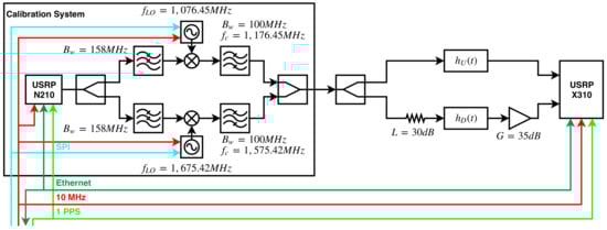
Figure 10.
Block diagram of the calibration system. is the frequency of the local oscillator (LO), is the −3 dB bandwidth, is the −3 dB cut-off frequency, L stands for attenuation, and G stands for gain.
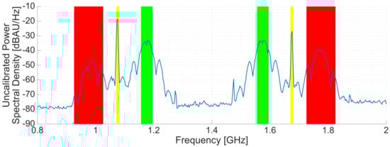
Figure 11.
Measured spectra of the transmitted calibration signal at L1/E1 frequency band (right), and at L5/E5a frequency band (left). In green, the region of the spectrum that will be used for calibration. The aliases of the up-conversion are highlighted in red. The local oscillator leakages are highlighted in yellow.
Figure 11 shows the spectra of the calibration signal around the L1/E1 frequency band (left) and the L5/E5a frequency band (right). The aliases of the up-conversion (in red), and the LO leakage (yellow) can be clearly seen in both figures. The region of the spectra that will be used to calibrate the instrument is highlighted in green. The PRN codes were generated at the highest IF possible in order to distance as much as possible the up-conversion aliases and the LO leakage respect to the useful frequency band.
Section 3 digs into the two-step calibration procedure.
2.6. Instrument Integration
All blocks except the arrays, the inclinometer, the GNSS antennas and the IMU are mounted inside a custom-made rack with three different floors (Figure 12) that measures 570 × 500 × 470 mm and weights 70 kg approximately. The top level has the GNSS receiver, the calibration system, all power supplies, and the Linux embedded system. The beamformers are attached in the middle level. There, the 19 cables coming from the arrays are connected to the beamformers. Additionally, there is an extra connector for the cable that connects the calibration system and that array (Figure 12, bottom right). From each beamformer, the 4 output cables go to the lower floor. The cables from the up-looking beamformer are connected directly to the SDRs. The cables of the down-looking beamformers are first connected to RF amplfiers. The bottom level has attached the gigabit ethernet switch, the Octoclock, the extra RF amplifiers for the down-looking RF chain, and the SDR. The inclinometer is attached to one of the sides of the rack, while the inertial measurement unit and the GNSS antennas are attached to the up-looking array.
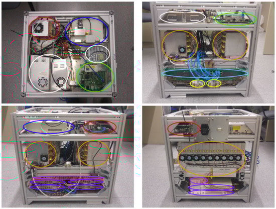
Figure 12.
MIR rack. The top floor of the rack has the embedded system (red), the power supplies (white), the calibration system (blue), and the GNSS receiver (green). The middle floor has the beamformers (orange). The lower floor has the Octoclock (magenta), the SDR (purple), the gigabit ethernet swithc (cyan), and the extra amplifiers for the down-looking RF chain (yellow).
3. Instrument Calibration
The calibration procedure is divided in two steps, a pre-calibration in an anechoic chamber, and the in-flight calibration.
3.1. Pre-Calibration
In the pre-calibration, the arrays and the beamformers are characterized. They do not need to be calibrated every time the instrument is turned on, but they should be calibrated from time to time. The pre-calibration has four steps. First, the array and the beamformers are characterized in the anechoic chamber using an externally transmitted signal that is received by the antennas. Then, they are characterized again injecting a signal through the calibration port. Next, from these two measurements, the difference between both paths is estimated, which will be called the “compensation parameters”. Last, once the instrument has been finished and all the final hardware is mounted, it is calibrated again through the calibration port using a vector network analyzer and the “compensation parameters”.
3.1.1. Step 1: Calibration through the Antenna
The received signals from the satellites follow the red path in Figure 13. The signal is propagated from the satellite (or the transmitting antenna inside the anechoic chamber) to the phase center of the antenna (), passes through the calibration switch () and through the vector modulator . The two last contributions and are the ones that must be calibrated. To conduct these measurements, an external antenna is required. In the MIR case, it was mounted in an anechoic chamber. The transmitting antenna was a reference antenna connected to the transmitting port of a vector network analyzer, whereas the receiving port was connected to the output of the beamformer.
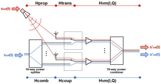
Figure 13.
Received and calibration signal’s paths to the receiver in one of the bands and beams.
The outcoming signal is
where is the transfer function measured by the VNA. In case one single vector modulator i has to be characterized, the rest of gains can be set to zero
As it can be seen, the offset contribution is always present and constant. In order to estimate the calibration parameters g, , L, and , it is required to estimate the vectors , , and O in Equation (4). For each vector modulator i, several transfer functions are measured setting N different pairs of values. The following linear system is obtained:
If more than three independent measurements are used, the system can be solved using the linear least squared method
This linear approximation requires a set of values that maintain the RF devices in the linear region. The MIR instrument uses
with . Once the system is solved, the contribution can be removed
where is the vector between the phase centers of the transmitting and the i receiving antenna, and is the wavelength.
Then, the calibration parameters (g and ), and the unbalance parameters of the vector modulator (L and ) of each RF chain are obtained from and as:
3.1.2. Step 2: Calibration through the Calibration Port
Since it is unpractical to periodically calibrate the instrument with an external antenna, even more if the instrument is mounted in an airplane, the instrument has a calibration port in each array (blue path in Figure 13). There, the calibration signal is split and distributed to the 19 RF Front-ends (). The calibration signal is coupled to the RF main line due to the switch finite isolation (), and then the signal follows the same route than the signal coming from the antennas through the rest of the RF chain ().
To conduct these measurements, the transmitting port of the anechoic chamber’s VNA was connected to the calibration port, whereas the receiving port was connected to the output of the beamformer. In the MIR case it was done just after the first calibration step, connecting to the calibration port the cable that fed the transmitting antenna.
The outgoing signal is in this case
Again, the system of Equation (12) has to be solved, but in this case the vector is
3.1.3. Step 3: Obtaining the Compensation Parameters
As aforementioned, the calibration through the calibration port is more practical than the calibration with an external reference antenna, but the calibration signal does not follow the same path that the signals that come from the satellites. It is proposed to measure the differences in the paths, so this path difference can be compensated in the calibration parameters obtained through the calibration port. From Figure 13, they can be defined as
Considering that they depend on a particular pair of values, it is instead proposed to compute them as
Note that the compensation parameters do not depend on the vector modulators, and therefore they will not change between beams of the same band.
3.1.4. Step 4: Re-Calibrating the Instrument
If any hardware after the calibration switch has changed or the instrument needs to be calibrated again, this can be done through the calibration port and then applying the “compensation parameters”. To do so, the instrument has to be first calibrated following the step 2 in Section 3.1.2 to obtain a new pair of , and then they are multiplied by the compensation parameter
where and must be used to compute the calibration parameters as explained in Equations (16)–(19). After that, the offsets in Equation (20) should be recalculated.
3.2. In-Flight Calibration
In the in-flight calibration it is estimated the random phase of the local oscillators for later compensation. Besides, during the pre-calibration, the gain of the elements was calibrated with respect to the elements of the same array, so it is required to perform a calibration between both arrays. To do so, a calibration signal is injected as explained in Section 3.2, and it is corrected in post-processing. In the MIR case, the power splitter and the cables that connect the calibration system to the calibration port were not pre-calibrated, so it they were characterized for later compensation.
In this step only one measurement per USRP is required to characterize the phase and gain between the up and down-looking channels. If a known gain G and phase are set to one element in the up and down-looking arrays for the same beam (that is, the same USRP), the phase and gain differences between the sampled signals is the phase and gain differences between channels. To estimate these differences a calibration signal is injected in the arrays and sampled with the USRPs for later processing and compensation.
The up-converted signal is injected in each RF Front-end. All vector modulators except the one corresponding to the central element of the array are disabled. The outcoming is sampled with the receiving SDRs. As for the normal operation mode, the calibration signals are sampled by beam pairs. In the calibration mode, however, the receiving USRP samples the signals at 10 Msps with 16 bits for the I and Q components. The sampled signal is
where is the periodic base-band transmitted calibration signal, is the up-conversion frequency, is the random phase of the transmitting local oscillator, is the equivalent base-band impulse response of the transmitting USRP, * is the convolution operator [19], h is the combined equivalent base-band impulse response of the Device Under Test (DUT), the splitting network after the calibration system, and the receiving USRP, is the band central frequency, is the base-band additive white Gaussian noise present in the channel, is the down-conversion frequency, and is the random phase of the receiving local oscillator. If the transfer functions of and are flat enough to state that , can be approximated to simplify Equation (27)
where and are the differences between the frequencies and the random phases of the local oscillators in the up and down conversion respectively, and , and have been abbreviated for simplicity.
First, the residual frequency difference between oscillators has to be compensated, otherwise the phase will not remain constant over time. To do so, is circularly cross-correlated with a length clean replica of the calibration signal . Then, the phase in the cross-correlation peak is used to estimate the frequency error between oscillators, as it is proven in Equation (A1) from Appendix A
where is the time length of the code, is the chip duration, is the convolution in the time domain, and is the Woodward Ambiguity Function (WAF) which for Binary Phase Shifting Keying (BPSK) codes can be approximated as [20]
where is the coherent integration time, and
If a simplified model of the transmitting impulse response is assumed, so that the channel behaves as a simplified model , so , according to Equation (A5) from Appendix A, Equation (29) becomes
The correlation peaks are located at , so that can be found by correlating the first of the sampled data. Then, the peak value is
The phase rotates due to the term . If the SNR is high enough, the phase can be used to estimate the term , and once the frequency error can be compensated in a similar way [21]. When the sampled signal is correlated in intervals of with the clean replica of the code, the spectrum of each interval is
In order to retrieve the modulus of the combined transfer functions, the spectra contribution of the PRN codes has to be removed. The Fourier transforms of the PRN codes are known and exhibit null values. Dividing by the code spectra will therefore result in an inaccurate estimation of the transfer functions and . It is therefore recommended to estimate and using the Barlett’s method [19]. To do so, each interval of the K intervals of the input signal is divided into M sub-intervals. The optimum number of sub-intervals to reduce the variance of the estimation of all three parameters was found empirically to be for the MIR instrument. Knowing the delay , these sub-intervals are cross-correlated with the corresponding part of the transmitted code. The M sub-intervals are then averaged to get a smoothed estimation of the spectra , which is used to estimate the transfer functions in Equation (35). Last, the K estimated transfer functions are averaged to reduce the impact of the noise .
The estimated transfer function of the up-looking and down-looking channels becomes:
where the subscripts u and d stand for the up- and down-looking channels, respectively. By dividing both transfer functions we obtain
which is used for the relative calibration between channels. Note that also includes the contributions of the power splitting network after the calibration system, and they have to be removed. To do so, these parts are measured using a 4-port vector network analyzer (Rohde-Schwarz ZVB-8).
Figure 14 shows the estimated for all intervals of one of RF chains using sub-intervals, and the estimated linearization. As it can be seen, the phase is linear, and the y-intercept points of the different intervals are similar, proving that the frequency error between local oscillators is successfully compensated, otherwise the phase (y-intercept point) will be rotating. The estimated phase was −29 with an standard deviation of 0.88. The estimated group delay was 15.26 ns with an standard deviation of 0.11 ns. The estimated gain was −7.14 dB with a geometric standard deviation of 0.1 dB.
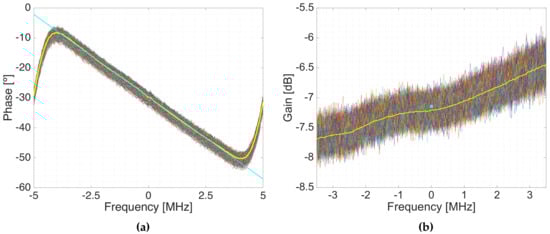
Figure 14.
Estimated phase (a) and gain (b) of the different intervals. The time averaged phase response estimation is plot in yellow, and the linear approximation in cyan. A value of was used. The time geometrically averaged amplitude of the transfer function is plot in yellow, and the geometric average gain is plot as a dot in cyan.
Three experiments were set to analyze the behavior of the system over time. These 3 experiments were conducted in different winter days in a room without heating, with 4 calibration measurements done in each experiment. Figure 15 shows the estimated phase between the direct and reflected RF chains for the 4 different USRPs (each one represented with a different color). As it can be seen, the phase remains constant, which proves that the frequency error between oscillators has been succesfully corrected. Figure 16 shows the group delay between RF chains, and Figure 17 shows the gain between channels. From these plots can be estimated that more than 150 min were required to heat up the instrument. Note that in a warmer environment the heating up time might be shorter.
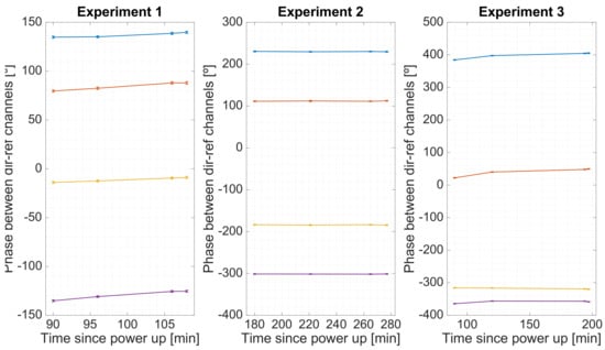
Figure 15.
Estimated phase between the direct and reflected RF channels for the four different USRPs during three sets of experiments. The lines show the drift between the estimations, and the markers are error bars.
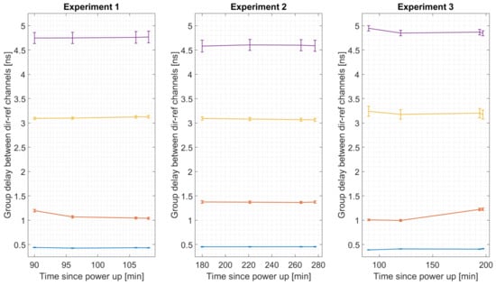
Figure 16.
Estimated group delay between the direct and reflected RF channels for the four different USRPs during three sets of experiments. The lines show the drift between the estimations, and the markers are error bars.
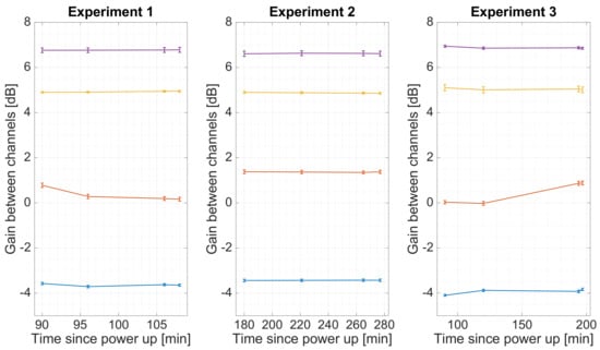
Figure 17.
Estimated gain between the direct and reflected RF channels for the four different USRPs during three sets of experiments. The lines show the drift between the estimations, and the markers are error bars. The mean and the standard deviation have been computed as geometric mean and geometric standard deviation.
4. Validation Results
This section describes the main experiments carried out to check that the instrument works properly prior to start any field campaign. First, during the pre-calibration in the anechoic chamber, some radiation patterns were measured, both with the instrument calibrated and uncalibrated, and the beam-steering capabilities were tested. Later on, the instrument was placed in the laboratory rooftop tracking GPS and Galileo satellites to ensure that the instrument is able to receive properly all the desired GNSS signals with proper power levels.
4.1. Calibration Impact and Measured Radiation Patterns
During the pre-calibration in the anechoic chamber (Figure 18), the beam-steering capabilities of the antenna arrays were also evaluated.
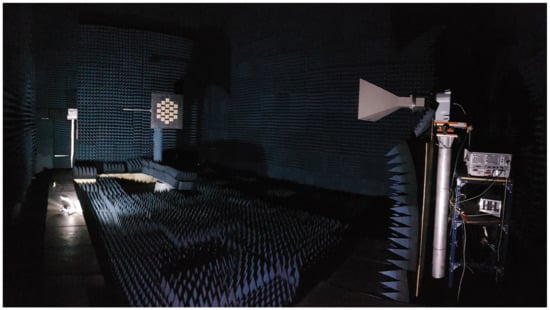
Figure 18.
MIR down-looking array being calibrated and measured at the Universitat Politècnica de Catalunya (UPC) anechoic chamber. The 19 elements MIR array is at the back left, while the transmitting reference horn antenna is at the front right. The transmitting antenna has linear polarization and can rotate along the boresight axis.
The beamformers and the arrays were calibrated following the procedure described in Section 3.1. Figure 19 shows the IQ gain circles explained in Section 2.2 of all vector modulators of an L1 beam before (left) and after calibrating (right). A red circle with the average gain has been drawn to ease the viewing of the improvement and the impact of the amplitude unbalance. The radii lines mark the parameter, which is where the gain circle starts to “rotate”. Before calibration, when setting a desired angle in the vector modulators, the achieved angle had an Root Mean Square (RMS) error of 13, at L1 and 16 at L5. After calibration, the RMS improves down to 4.9 and 4.2, respectively. Similarly, amplitude errors were corrected from 0.55 dB and 0.11 dB to 0.02 dB and 0.03 dB at L1 and L5 respectively. The approximated impact of these errors in the array directivity are shown in Table 3 [22].
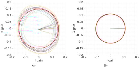
Figure 19.
IQ gain circles before (a) and after calibration (b). The radii lines mark where the circle starts to “rotate”. A red circle with average radius has been added to ease the viewing the effect of the amplitude unbalance.
Table 3.
Beamformer inaccuracy impact in the array directivity before and after calibration.
Figure 20 shows the impact of the calibration in the radiation pattern when the down-looking array (LHCP) was pointing to the boresight of the antenna both at L1/E1 (top) and at L5/E5 (bottom) frequency bands. The calibration improves the nulls of the radiation pattern in both bands. Besides, the uncalibrated beam in L1 is slightly tilted towards the right, which is corrected due to the calibration.
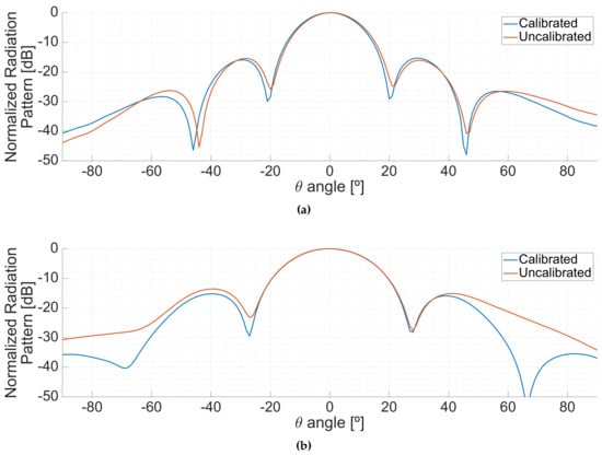
Figure 20.
Effect of the calibration in the radiation patterns. Planar cuts in the plane at L1/E1 (a) and L5/E5 (b).
After the beamformer calibration, the beam-steering capabilities were tested by tilting the beams from the boresight of the antenna to one of the sides, and some cuts of the antenna radiation pattern were measured. Figure 21 shows the antenna radiation patterns measured in the same plane where the beams were tilted, at L1/E1 (top), and at L5/E5 (bottom) frequency bands. The experiment was carried out for off-boresight angles (OBA) from 0 to 50 in steps of 10. As it can be seen, the maximum decreases as the beam is pointed far from the boresight due to the antenna radiation pattern of the individual elements, and due to the smaller projected area of the array. This loss of directivity was measured as well in order to be compensated while conducting scatterometric measurements and it can be seen in Figure 22. Similarly, the phase dependence to the direction of arrival for altimetric measurements was also measured.
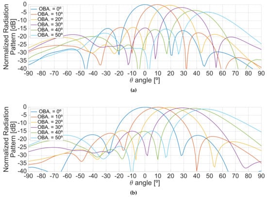
Figure 21.
Planar cuts of the radiation pattern along the plane when tilting the beam in the same plane for different off-boresight pointing angles, at the L1/E1 (a) and L5/E5 (b) frequency bands.
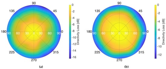
Figure 22.
Directivity loss as a function of the pointing direction at L1/E1 (a), and at L5/E5 (b), for the down-looking array.
The difficulties to power the instrument complicated the measurements of the back part of the radiation patterns. The back lobes were measured only pointing to the boresight, and are shown in Figure 23.
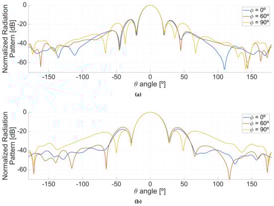
Figure 23.
Azimuthal cuts of the full radiation pattern pointing to the boresight of the antenna, at the L1/E1 (a) and L5/E5 (b) frequency bands.
It was therefore complicated to accurately estimate the directivity of the array since only the frontal hemisphere of the radiattion pattern was measured (Figure 24). The estimated directivities for both arrays while pointing to the boresight can be seen in Table 2.
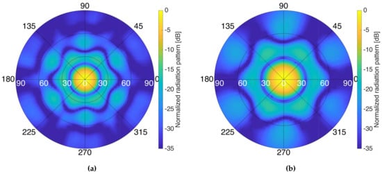
Figure 24.
Frontal hemisphere of the measured radiation pattern of the down-looking array, at the L1/E1 (a) and at L5/E5 (b) frequency bands.
Figure 25 shows different antenna radiation pattern cuts when pointing to an off-boresight angle of 35. The side lobe levels are lower than 12 dB and 14 dB at L1/E1 and L1/E1 frequency bands, respectively.
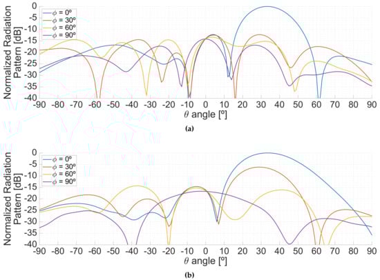
Figure 25.
Side lobes for different azimuthal cuts of the antenna pattern when pointing to an off-boresight angle of 35 at the L1/E1 (a) and L5/E5 (b) frequency bands, respectively.
4.2. Outdoor Experiments
Several experiments were carried out in the rooftop of the laboratory to ensure the proper working of the instrument. The first one aimed to check that the instrument was able to retrieve data from all systems and frequency bands with enough power. To do so, the up-looking array was placed with a random orientation with respect to the North (Figure 26), pointing to GPS and Galileo satellites at both L1/E1 and at L5/E5 frequency bands. The received signals were sampled and stored at 16 bits and 20 Msps, and cross-correlated with clean replicas of the PRN codes. Figure 26 also shows four retrieved different waveforms for GPS and Galileo in both frequency bands. The correlation peaks are displayed in the time origin of a single figure to for easier intercomparison. The experiment also aimed at checking if extra gain was required to reach the sensitivity of the SDR and to take advantage of the whole dynamic range of the Analog to Digital Converters (ADC), which was not. In order to check if more gain was required for the down-looking RF chain, attenuators were placed before the SDRs in order to determine the sensitivity level. Since the reflected signals are expected to be 0–30 dB weaker than those collected by the up-looking RF chain, two extra RF amplifiers with a total gain of ≈35 dB were added just before the SDRs in the down-looking chains.
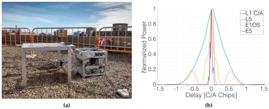
Figure 26.
MIR up-looking array and rack during the rooftop experiments (a), and retrieved waveforms from GPS and Galileo satellites in both L1/E1 and L5/E5 frequency bands (b) during the rooftop experiments [23].
Later on, the satellite selection algorithm was tested by leaving the instrument tracking the optimum satellites and monitoring the C/N0 at the output of the beamformers. To do so, the outputs of the L1-1 and L1-2 beams were connected to a dual-antenna GNSS receiver capable of tracking GPS and GLONASS satellites (the selection of Galileo satellites was deactivated in order to be able to track the pointed satellites). The C/N0 of all satellites was monitored for a long time. Figure 27 shows the C/N0 tracked in the L1-1 beam (top) and the L1-2 beam (bottom). As it can be seen, the tracked satellite receives more power than the others. The satellite selection algorithm was set to chose the optimum satellites every 5 min. Two changes in the tracked satellites can be observed in the figure, where the C/N0 of the satellites drops or raises suddenly when the algorithm decided to track a different satellite.
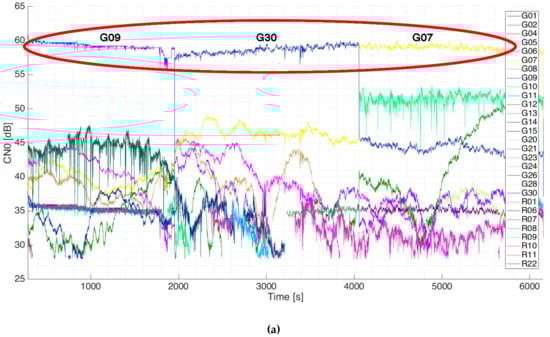
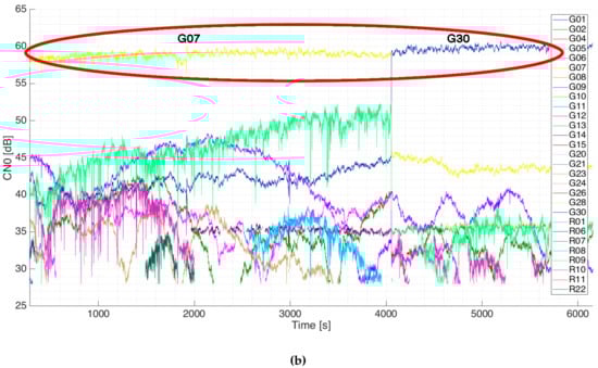
Figure 27.
Tracked C/N0 in the L1-1 beam (a) and L1-2 beam (b), both red circled, during the experiment in the laboratory rooftop [24].
5. Summary
This work has presented the MIR instrument, a new airborne GNSS-Reflectometer that has been built during the last years in Universitat Politècnica de Catalunya to emulate the behavior of the future PARIS-IoD [25], GNSS rEflectometry, Radio Occultation, and Scatterometry onboard the International Space Station (GEROS-ISS) [26], or GNSS Transpolar Earth Reflectometry exploriNg system (G-TERN) [27] missions thanks to its large directive antennas, multi-beam and dual-frequency (L1/E1 and L5/E5a) capabilities. Obtaining the “compensation parameters” eases the later periodical instrument calibration by injecting PRN signals during operations, which have been proved useful to calibrate the instrument.
The system’s analog beamformers use vector modulators to change the amplitude and phase of the received signals by the antennas. A 4-model parameter model is proposed to characterize the vector modulators. This model in conjunction with the proposed calibration procedure reduces the amplitude errors in the beamforming from 0.55 dB and 0.11 dB to 0.03 dB and 0.02 at L1/E1 and at L5/E5a, respectively. The phase errors are reduced in the beamforming from 13 and 16 to 4.9 and 4.2 at L1/E1 and at L5/E5a, respectively. The consequent loss of directivity in the array is therefore reduced from 0.28 dB and 0.34 dB to 0.03 dB and 0.02 dB at L1/E1 and at L5/E5a, respectively.
The array directivity pointing to the boresight reaches 20 dB and 18 dB at L1/E1 and at L5/E5a, respectively. The measured beamwidth pointing to the boresight is 17 and 23 at L1/E1 and at L5/E5a, respectively. When the beam is steered 35 off-boresight, the beamwidth increases up to 20 and 27 at L1/E1 and at L5/E5a, respectively, and the side lobes are lower than 12 dB and 14 dB, respectively. The beamsteering capabilites have been demonstrated up to 50 with a maximum directivity loss of 5 dB at L1, larger than the desired 35. The automatic satellite tracking capabilities have also been proved.
Future work involves field experiments, development of data processing algorithms, implementation in the URSPs of these algorithms for real-time processing, and the implementation in the USRPs of the fourth step of the pre-calibration and the in-flight calibration to calibrate and compensate the component aging.
Author Contributions
R.O., D.P., J.Q., A.C. and H.P. conceived the instrument; R.O. designed, implemented, integrated and tested all the hardware; R.O., D.P., J.Q. and A.C. designed the calibration procedure; R.O. calibrated the instrument; R.O. and D.P. performed the validation experiments; R.O. wrote the paper; and D.P., A.C. and H.P. revised the manuscript.
Funding
This work was supported by the Spanish Ministry of Economy and Competitiveness and FEDER EU under the project “AGORA: Técnicas Avanzadas en Teledetección Aplicada Usando Señales GNSS y Otras Señales de Oportunidad” (MINECO/FEDER) ESP2015-70014-C2-1-R by the Agencia Estatal de Investigación, and the grant for recruitment of early-stage research staff FI-DGR 2015 of the AGAUR—Generalitat de Catalunya (FEDER). Spain, and Unidad de Excelencia María de Maeztu MDM-2016-0600, and to Prof. Camps ICREA Academia 2015 award of the Generalitat de Catalunya.
Acknowledgments
Special thanks to Sebastià Blanch for his help in the array calibration and the antenna radiation pattern measurements.
Conflicts of Interest
The authors declare no conflict of interest. The founding sponsors had no role in the design of the study; in the collection, analyses, or interpretation of data; in the writing of the manuscript, and in the decision to publish the results.
Abbreviations
The following abbreviations are used in this manuscript:
| ADC | Analog-to-Digital Converter |
| BPSK | Binary Phase Shifting Keying |
| −3 dB Bandwidth | |
| cGNSS-R | conventional Global Navigation Satellite Systems—Reflectometry |
| COTS | Commercial Off-The-Shelf |
| DAC | Digital-to-Analog Converter |
| DCM | Direction Cosine Matrix |
| DUT | Device Under Test |
| ECEF | Earth Centered Earth Fixed |
| Cut-off frequency at −3 dB | |
| LO frequency | |
| FM | Frequency Modulation |
| G | Gain |
| GEROSS-ISS | GNSS rEflectometry, Radio Occultation and Scatterometry onboard the International Space Station |
| GLONASS | GLObalnaya NAvigatsionnaya Sputnikovaya Sistema |
| GNSS | Global Navigation Satellite Systems |
| GNSS-R | Global Navigation Satellite Systems—Reflectometry |
| GPS | Global Positioning System |
| GPS-DO | GPS Disciplined Oscillator |
| GSM | Global System for Mobile communications |
| G-TERN | GNSS Transpolar Earth Reflectometry exploriNg system |
| I | In-phase component |
| IF | Intermediate Frequency |
| iGNSS-R | interferometric Global Navigation Satellite Systems—Reflectometry |
| IMU | Inertial Measurement Unit |
| L | Losses, attenuation |
| LHCP | Left Hand Circular Polarized |
| LNA | Low Noise Amplifier |
| LO | Local Oscillator |
| MIR | Microwave Interferometric Reflectometer |
| Msps | Mega Samples Per Second |
| NED | North East Down |
| NF | Noise Figure |
| PARIS-IoD | PAssive Reflectometry and Interferometry System In-orbit Demonstration |
| PPS | Pulse Per Second |
| PRN | PseudoRandom Noise |
| Q | Quadrature phase component |
| RF | Radio Frequency |
| RFI | Radio Frequency Interference |
| RMS | Root Mean Square |
| RHCP | Right Hand Circular Polarized |
| SAW | Surface Acoustic Wave |
| SBAS | Satellite-Based Augmentation Systems |
| SDR | Software Defined Radio |
| SNR | Signal-to-Noise Ratio |
| Chip time of a PRN code | |
| Coherent integration time | |
| PRN time length | |
| USRP | Universal Software Radio Peripheral |
| VNA | Vector Network Analyzer |
| Wavelength of GPS at L1 central frequency (19.04 cm) | |
| Wavelength of GPS at L5 central frequency (25.5 cm) |
Appendix A. Formulas Used in the Derivation of the Cross-Correlation Function for the Calibration Process
The cross-correlation function of the sampled calibration signal is
If it is assumed a simplified model of the channel , and the model for the WAF defined in Equation (30), the cross-correlation of the calibration signal becomes
References
- Hall, C.; Cordey, R. Multistatic Scatterometry. In Proceedings of the International Geoscience and Remote Sensing Symposium: Remote Sensing: Moving Toward the 21st Century, Edinburg, UK, 12–16 September 1988; Volume 1, pp. 561–562. [Google Scholar]
- Martin-Neira, M. A Passive Reflectometry and Interferometry System (PARIS): Application to Ocean Altimetry. ESA J. 1993, 17, 331–355. [Google Scholar]
- Onrubia, R.; Querol, J.; Pascual, D.; Alonso-Arroyo, A.; Park, H.; Camps, A. DME/TACAN Impact Analysis on GNSS Reflectometry. IEEE J. Sel. Top. Appl. Earth Obs. Remote Sens. 2016, 9, 4611–4620. [Google Scholar] [CrossRef]
- Pascual, D.; Park, H.; Onrubia, R.; Arroyo, A.A.; Querol, J.; Camps, A. Crosstalk Statistics and Impact in Interferometric GNSS-R. IEEE J. Sel. Top. Appl. Earth Obs. Remote Sens. 2016, 9, 4621–4630. [Google Scholar] [CrossRef]
- Katzberg, S.; Garrison, J. Utilizing GPS To Determine Ionospheric Delay over the Ocean; NASA Technical Memorandum 4750; NASA: Greenbelt, MD, USA, 1996. [Google Scholar]
- European Union. European GNSS (Galileo) Open Service Signal-In-Space Interface Control Document (OS SIS ICD); Technical Report; European Union: Brussels, Belgium, 2014. [Google Scholar]
- Pascual, D.; Camps, A.; Martin, F.; Park, H.; Arroyo, A.A.A.; Onrubia, R. Precision Bounds in GNSS-R Ocean Altimetry. IEEE J. Sel. Top. Appl. Earth Obs. Remote Sens. 2014, 7, 1416–1423. [Google Scholar] [CrossRef]
- Onrubia, R.; Camps, A. Antena Multibanda Tipo Parche con Sistema de Alimentación Cruzada. Spain Patent ES2540161B2, 8 October 2015. [Google Scholar]
- Alonso-Arroyo, A.; Camps, A.; Monerris, A.; Rudiger, C.; Walker, J.P.; Onrubia, R.; Querol, J.; Park, H.; Pascual, D. On the Correlation Between GNSS-R Reflectivity and L-Band Microwave Radiometry. IEEE J. Sel. Top. Appl. Earth Obs. Remote Sens. 2016, 9, 5862–5879. [Google Scholar] [CrossRef]
- Analog Devices ADL5390 Rev. A. Available online: http://www.analog.com/media/en/technical-documentation/data-sheets/ADL5390.pdf (accessed on 6 September 2018).
- Wandboard Quad (I.MX6). Available online: https://www.wandboard.org/products/wandboard/WB-IMX6Q-BW/ (accessed on 25 October 2018).
- Trimble BD982. Available online: https://www.trimble.com/gnss-inertial/bd982.aspx (accessed on 8 January 2018).
- Onrubia, R.; Garrucho, L.; Pascual, D.; Park, H.; Querol, J.; Alonso-Arroyo, A.; Camps, A. Advances in the MIR instrument: Integration, control subsystem and analysis of the flight dynamics for beamsteering purposes. In Proceedings of the 2015 IEEE International Geoscience and Remote Sensing Symposium (IGARSS), Milan, Italy, 26–31 July 2015; Volume 2015, pp. 4765–4768. [Google Scholar]
- GPS. NAVSTAR GPS Control Segment to User Support Community Interfaces; ICD-GPS-870; Interface Control Working Group, Navstar GPS Joint Program Office: El Segundo, CA, USA, 2013. [Google Scholar]
- Seika NG-4. Available online: http://www.seika.de/english/htmle/NGe.htm (accessed on 7 November 2018).
- 9 Degrees of Freedom—Razor IMU. Available online: https://www.sparkfun.com/products/retired/10736 (accessed on 25 October 2018).
- Ettus Research USRP X310. Available online: https://www.ettus.com/content/files/X300_X310_Spec_Sheet.pdf (accessed on 6 September 2018).
- Ettus Research Octoclock. Available online: https://www.ettus.com/content/files/Octoclock_Spec_Sheet.pdf (accessed on 6 September 2018).
- Proakis, J.G.; Manolakis, D.G. Digital Signal Processing Principles, Algorithms and Applications; Pearson: San Antonio, TX, USA, 1996. [Google Scholar]
- Zavorotny, V.U.; Gleason, S.; Cardellach, E.; Camps, A. Tutorial on remote sensing using GNSS bistatic radar of opportunity. IEEE Geosci. Remote Sens. Mag. 2014, 2, 8–45. [Google Scholar] [CrossRef]
- Querol, J. Radio Frequency Interference Detection and Mitigation Techniques for Navigation and Earth Observation. Ph.D. Thesis, Universitat Politècnica de Catalunya, Barcelona, Spain, 2018; pp. 196–200. [Google Scholar]
- Camps, A.; Park, H.; Valencia i Domenech, E.; Pascual, D.; Martin, F.; Rius, A.; Ribo, S.; Benito, J.; Andres-Beivide, A.; Saameno, P.; et al. Optimization and Performance Analysis of Interferometric GNSS-R Altimeters: Application to the PARIS IoD Mission. IEEE J. Sel. Top. Appl. Earth Obs. Remote Sens. 2014, 7, 1436–1451. [Google Scholar] [CrossRef]
- Onrubia, R.; Pascual, D.; Querol, J.; Park, H.; Camps, A.; Rudiger, C.; Walker, J. Preliminary End-to-End Results of the MIR Instrument: the Microwave Interferometric Reflectometer. In Proceedings of the IGARSS 2018—2018 IEEE International Geoscience and Remote Sensing Symposium, Valencia, Spain, 22–27 July 2018; pp. 2027–2030. [Google Scholar]
- Onrubia, R.; Pascual, D.; Querol, J.; Park, H.; Camps, A. Beamformer characterization of the MIR instrument: The microwave interferometric reflectometer. In Proceedings of the 2017 IEEE International Geoscience and Remote Sensing Symposium (IGARSS), Fort Worth, TX, USA, 23–28 July 2017; Volume 2017, pp. 5026–5029. [Google Scholar]
- Martin-Neira, M.; D’Addio, S.; Buck, C.; Floury, N.; Prieto-Cerdeira, R. The PARIS Ocean Altimeter In-Orbit Demonstrator. IEEE Trans. Geosci. Remote Sens. 2011, 49, 2209–2237. [Google Scholar] [CrossRef]
- Wickert, J.; Andersen, O.; Beyerle, G.; Chapron, B.; Cardellach, E.; D’Addio, S.; Foerste, C.; Gommenginger, C.; Gruber, T.; Helm, A.; et al. GEROS-ISS: Innovative GNSS Reflectometry/Occultation Payload Onboard the International Space Station for the Global Geodetic Observing System; American Geophysical Union: Washington, DC, USA, 2013. [Google Scholar]
- Cardellach, E.; Wickert, J.; Baggen, R.; Benito, J.; Camps, A.; Catarino, N.; Chapron, B.; Dielacher, A.; Fabra, F.; Flato, G.; et al. GNSS Transpolar Earth Reflectometry exploriNg System (G-TERN): Mission Concept. IEEE Access 2018, 6, 13980–14018. [Google Scholar] [CrossRef]
© 2019 by the authors. Licensee MDPI, Basel, Switzerland. This article is an open access article distributed under the terms and conditions of the Creative Commons Attribution (CC BY) license (http://creativecommons.org/licenses/by/4.0/).