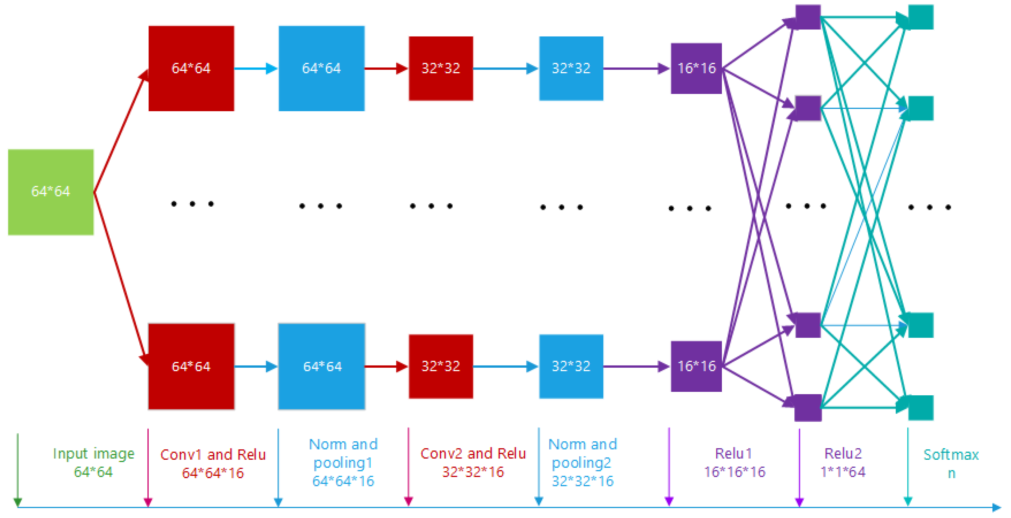
Figure 1.
Assembled CNN architecture.
Figure 1.
Assembled CNN architecture.
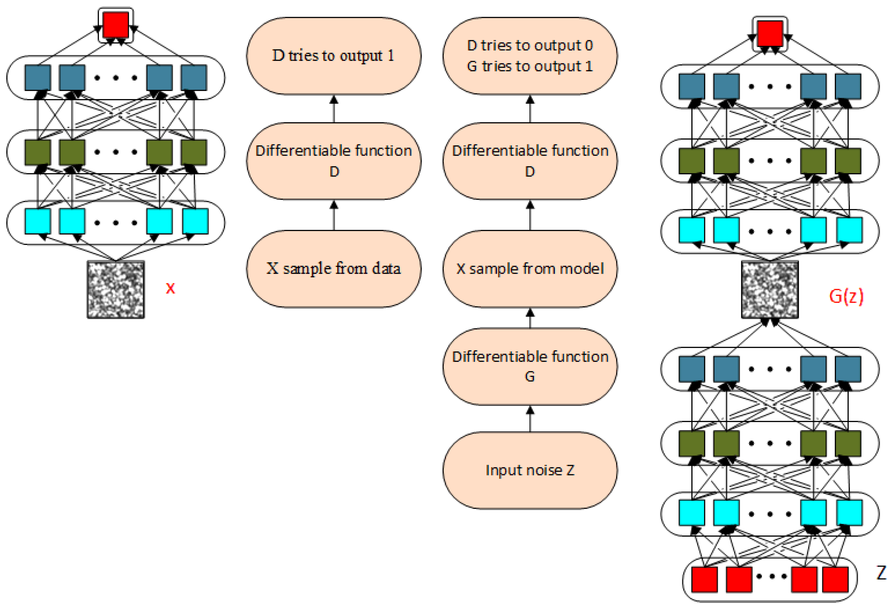
Figure 2.
Schematic of a GAN.
Figure 2.
Schematic of a GAN.
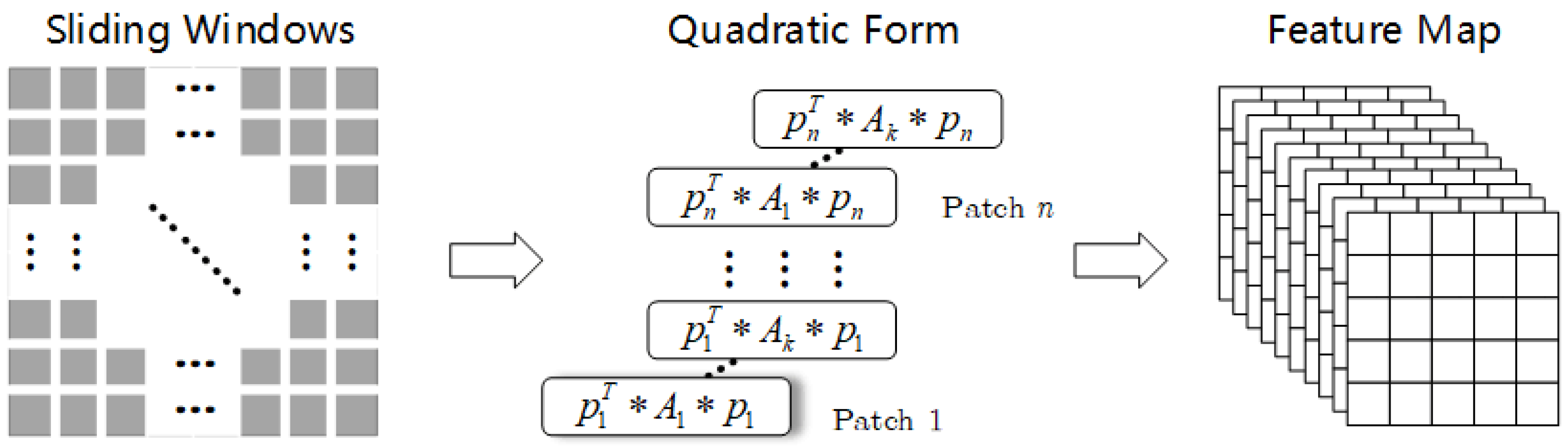
Figure 3.
Quadratic operation.
Figure 3.
Quadratic operation.
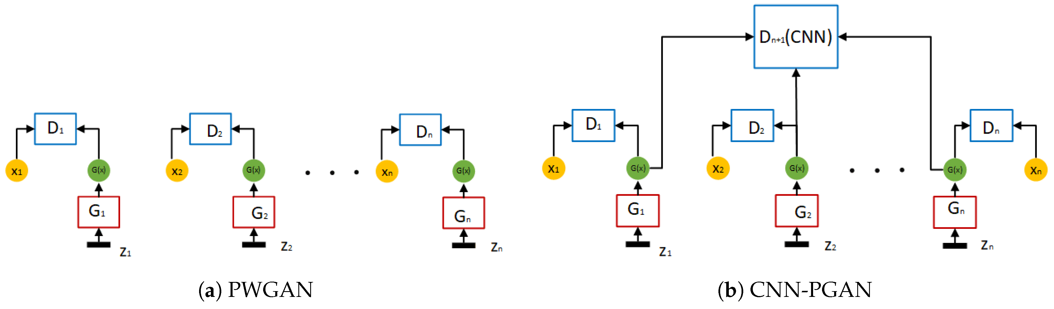
Figure 4.
Two different architectures of our proposed GAN.
Figure 4.
Two different architectures of our proposed GAN.
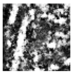
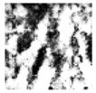
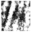
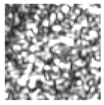
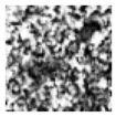
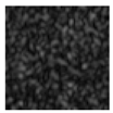
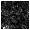
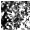
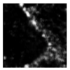
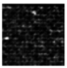
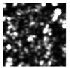
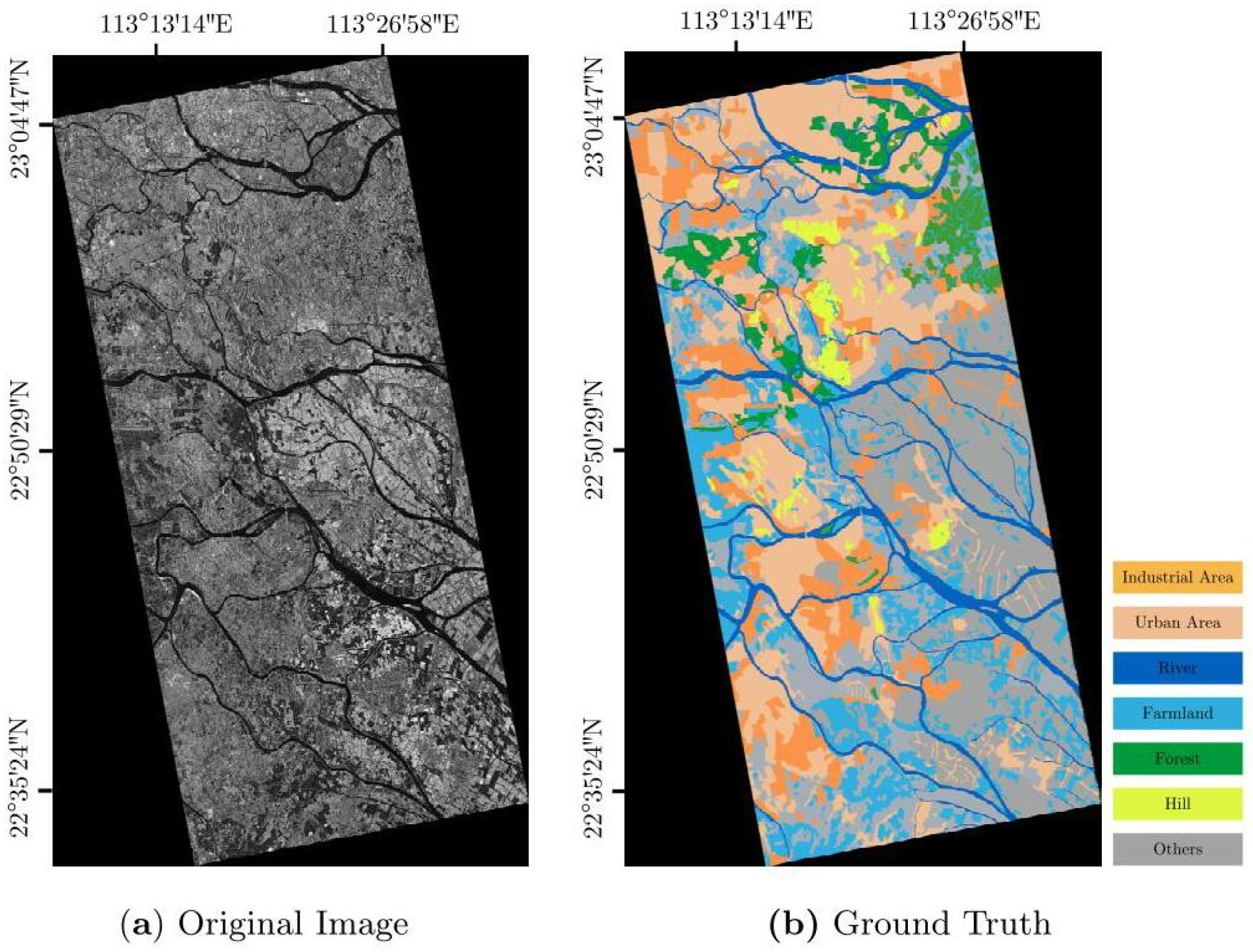
Figure 5.
DataSet1 (7 categories): single-polarized (VV) data acquired by TerraSAR-X over Guangdong, China (intensity image).
Figure 5.
DataSet1 (7 categories): single-polarized (VV) data acquired by TerraSAR-X over Guangdong, China (intensity image).
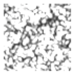
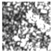
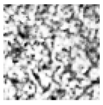
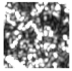
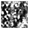
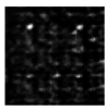
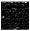
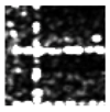
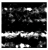
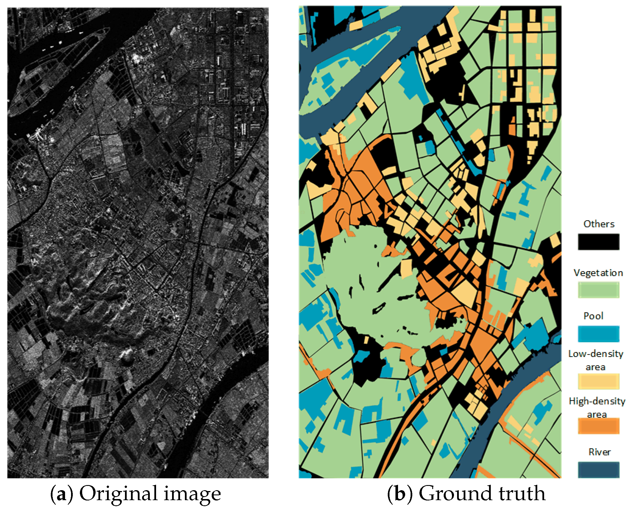
Figure 6.
DataSet2 (there are 6 categories, but only 5 are considered).
Figure 6.
DataSet2 (there are 6 categories, but only 5 are considered).
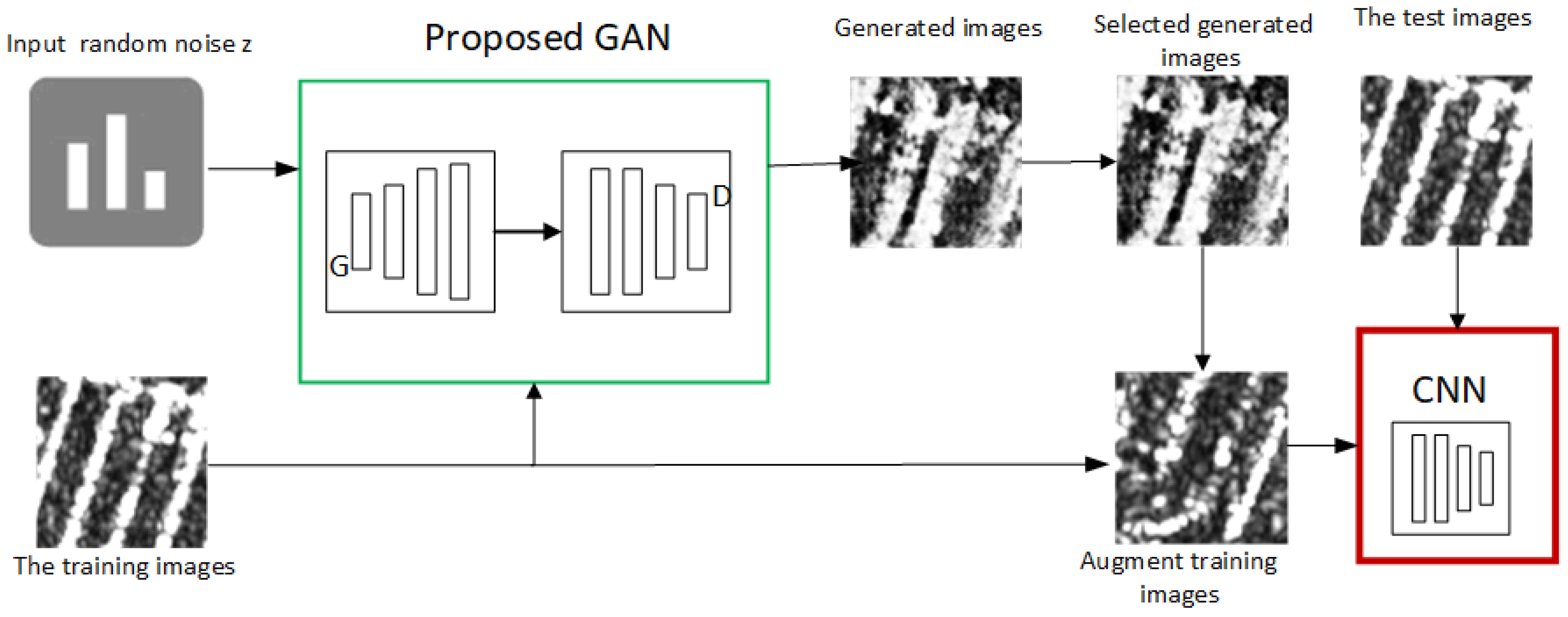
Figure 7.
Overview of our framework.
Figure 7.
Overview of our framework.
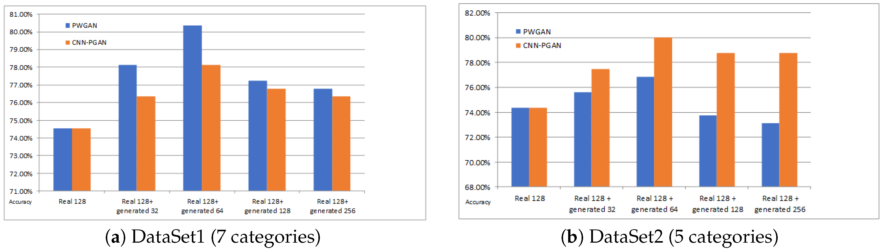
Figure 8.
The accuracy for different amounts of generated data for training on DataSet1 and DataSet2. The blue bar and the yellow bar indicate the classification accuracies of PGAN and CNN-PGAN, respectively. The first column is the classification result on the real 128 training images. The second, third, fourth, and fifth columns are the results of training data augmentation using 32, 64, 128, and 256 generated images, respectively.
Figure 9.
The classification result of different numbers of real images for training the entire network on DataSet1.
Figure 9.
The classification result of different numbers of real images for training the entire network on DataSet1.
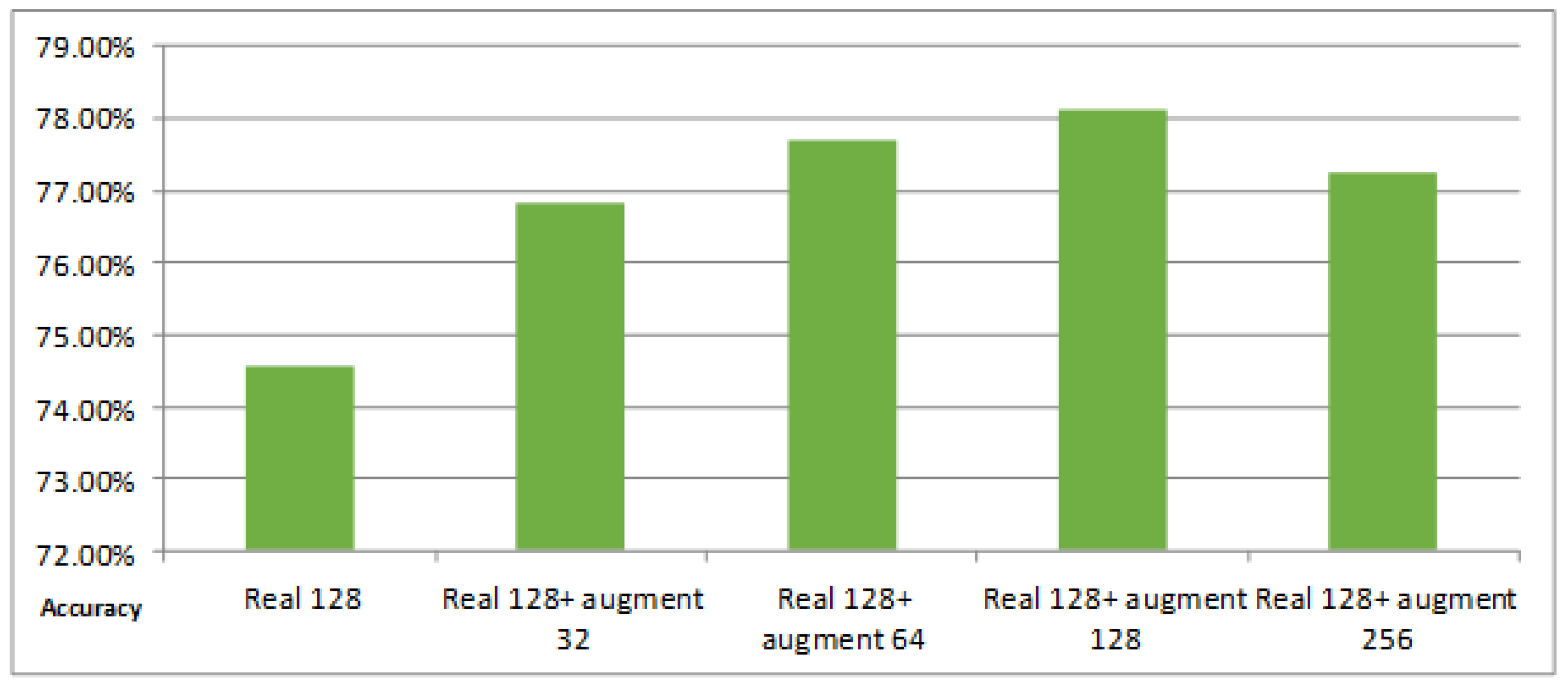
Figure 10.
The classification result of different numbers of augmented training data for DataSet1. The first column is the classification result on the real 128 training images. The second, third, fourth, and fifth columns are the results of training data augmentation using 32, 64, 128, and 256 images augmented by the simple augmentation strategy, respectively.
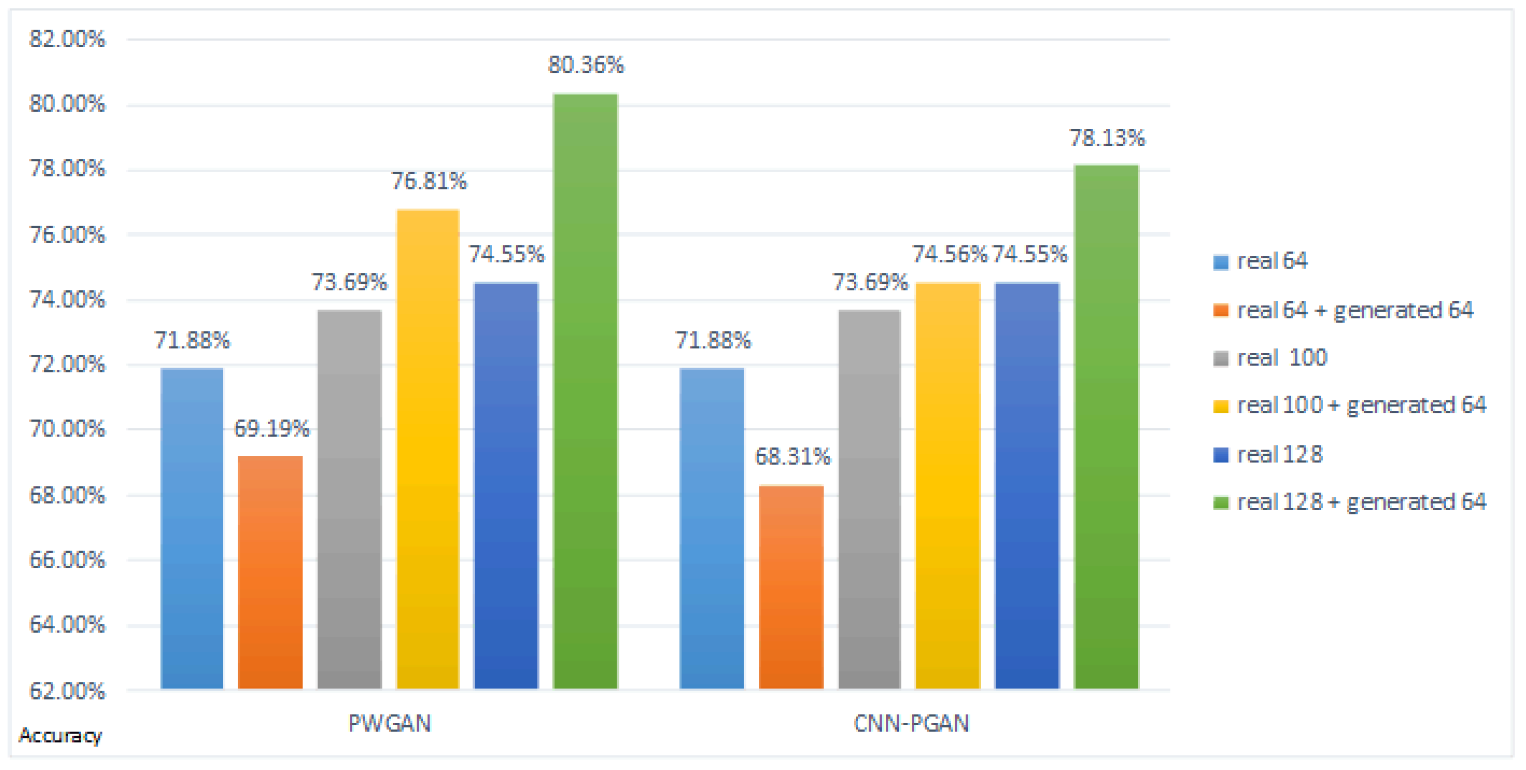
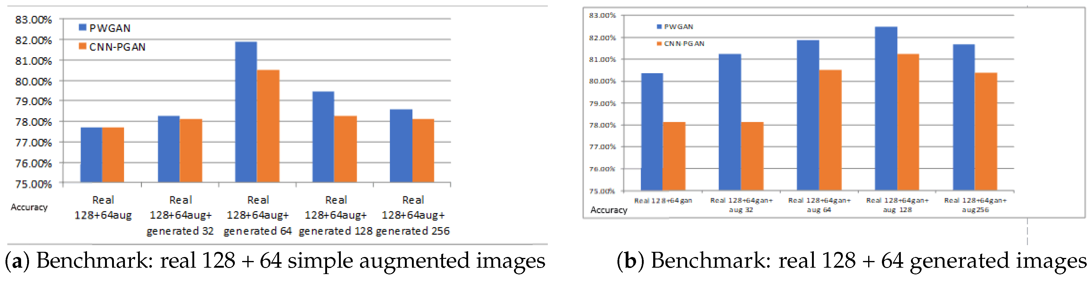
Figure 11.
The accuracy for different training datasets. The blue bar and the yellow bar indicate the classification accuracies of PWGAN and CNN-PGAN, respectively. (a) The first column is the classification result on the training dataset (128 real images and 64 augmented images). The second, third, fourth, and fifth columns are the results of training data augmentation using 32, 64, 128, and 256 generated images, respectively; (b) The first column is the classification result on the training dataset (128 real images and 64 augmented images). The second, third, fourth, and fifth columns are the results of training data augmentation using 32, 64, 128, and 256 augmented images, respectively. The test set is always the same.
Table 1.
Summary table of SAR image parameter estimation.
Table 1.
Summary table of SAR image parameter estimation.
| Distribution Type | Distribution Model | Parameter | Expression |
|---|
| Empirical distribution | Lognormal distribution | , | =
= |
| Weibull distribution | c, b | |
| Fisher distribution | M, | |
| Prior distribution | Rayleigh distribution | b | |
| Gamma distribution | | |
| K distribution | , | |
Table 2.
The settings of the CNN.
Table 2.
The settings of the CNN.
| Layer Type | Image Size | Feature Maps | Kernel Size | Stride |
|---|
| Input layer | 64 × 64 | 1 | - | - |
| Convolution + ReLU | 64 × 64 | 16 | 3 × 3 | 1 |
| Ma× pooling | 64 × 64 | 16 | 3 × 3 | 2 |
| Convolution + ReLU | 32 × 32 | 16 | 3 × 3 | 1 |
| Ma× pooling | 32 × 32 | 16 | 3 × 3 | 2 |
| Fully connected | 16 × 16 | 16 | - | - |
| Fully connected | 1 | 64 | - | - |
| Output | 1 | 7 | - | - |
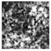
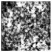
Table 3.
DataSet1: The original images and the images generated by PWGAN.
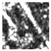
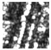
Table 4.
DataSet2: The original images and the images generated by CNN-PGAN.
Table 5.
The class-specific accuracy (%) and OA (Overall Accuracy) of different methods for DataSet1. DCGAN, Deep Convolutional GAN; WGAN, Wasserstein GAN.
Table 5.
The class-specific accuracy (%) and OA (Overall Accuracy) of different methods for DataSet1. DCGAN, Deep Convolutional GAN; WGAN, Wasserstein GAN.
| Class | CNN | AlexNet | DCGAN + CNN | WGAN + CNN | PWGAN | CNN-PGAN |
|---|
| 0 | 75 | 71.88 | 71.88 | 78.13 | 81.25 | 78.13 |
| 1 | 75 | 71.88 | 75 | 78.13 | 81.25 | 78.13 |
| 2 | 78.13 | 75 | 78.13 | 81.25 | 84.38 | 81.25 |
| 3 | 62.5 | 68.75 | 59.38 | 62.5 | 65.63 | 65.63 |
| 4 | 81.25 | 78.13 | 81.25 | 84.38 | 84.38 | 84.38 |
| 5 | 90.63 | 93.75 | 87.5 | 93.75 | 100 | 96.88 |
| 6 | 59.38 | 59.38 | 59.38 | 62.5 | 65.63 | 62.5 |
| OA | 74.55 | 74.11 | 73.21 | 77.23 | 80.36 | 78.13 |
Table 6.
The class-specific accuracy (%) and OA of different methods for DataSet2.
Table 6.
The class-specific accuracy (%) and OA of different methods for DataSet2.
| Class | CNN | AlexNet | DCGAN + CNN | WGAN + CNN | PWGAN | CNN-PGAN |
|---|
| 0 | 65.63 | 62.5 | 62.5 | 65.63 | 68.75 | 75 |
| 1 | 78.13 | 81.25 | 78.13 | 81.25 | 84.38 | 84.38 |
| 2 | 84.38 | 81.25 | 81.25 | 81.25 | 84.38 | 87.5 |
| 3 | 75 | 75 | 71.88 | 78.13 | 75 | 78.13 |
| 4 | 68.75 | 68.75 | 68.75 | 68.75 | 71.88 | 75.0 |
| OA | 74.38 | 73.75 | 72.5 | 75 | 76.88 | 80.0 |
Table 7.
Classification confusion matrix (ratio) for DataSet1 by using CNN only.
Table 7.
Classification confusion matrix (ratio) for DataSet1 by using CNN only.
| | 0 | 1 | 2 | 3 | 4 | 5 | 6 |
|---|
| 0 | 0.7500 | 0.0625 | 0.0313 | 0.125 | 0 | 0 | 0.0312 |
| 1 | 0.0313 | 0.7500 | 0.0937 | 0.0313 | 0.0312 | 0.0312 | 0.0313 |
| 2 | 0 | 0.0313 | 0.7813 | 0.0312 | 0.0937 | 0 | 0.0312 |
| 3 | 0.2187 | 0.0625 | 0.0313 | 0.6250 | 0 | 0 | 0.0625 |
| 4 | 0 | 0.0313 | 0.125 | 0 | 0.8125 | 0 | 0.0312 |
| 5 | 0 | 0.0312 | 0 | 0 | 0 | 0.9063 | 0.0625 |
| 6 | 0.0313 | 0.0625 | 0.0312 | 0.1250 | 0.1250 | 0 | 0.5938 |
Table 8.
Classification confusion matrix (ratio) for DataSet1 by using the PWGAN.
Table 8.
Classification confusion matrix (ratio) for DataSet1 by using the PWGAN.
| | 0 | 1 | 2 | 3 | 4 | 5 | 6 |
|---|
| 0 | 0.8125 | 0.0313 | 0.0313 | 0.0937 | 0 | 0 | 0.0312 |
| 1 | 0.0312 | 0.8125 | 0.0625 | 0.0313 | 0.0312 | 0 | 0.0313 |
| 2 | 0 | 0.0313 | 0.8438 | 0.0312 | 0.0937 | 0 | 0 |
| 3 | 0.156 | 0.0625 | 0.0313 | 0.6563 | 0 | 0 | 0.0312 |
| 4 | 0 | 0.0313 | 0.0937 | 0 | 0.8438 | 0 | 0.0312 |
| 5 | 0 | 0 | 0 | 0 | 0 | 1.0000 | 0 |
| 6 | 0.0313 | 0.0625 | 0.0312 | 0.0937 | 0.1250 | 0 | 0.6563 |
Table 9.
Classification confusion matrix (ratio) for DataSet1 by using CNN-PGAN.
Table 9.
Classification confusion matrix (ratio) for DataSet1 by using CNN-PGAN.
| | 0 | 1 | 2 | 3 | 4 | 5 | 6 |
|---|
| 0 | 0.7813 | 0.0313 | 0.0313 | 0.1249 | 0 | 0 | 0.0312 |
| 1 | 0.0312 | 0.7813 | 0.0625 | 0.0313 | 0.0312 | 0 | l|0.0313 |
| 2 | 0 | 0.0313 | 0.8125 | 0.0312 | 0.0937 | 0 | 0 |
| 3 | 0.2187 | 0.0625 | 0.0313 | 0.6563 | 0 | 0 | 0.0312 |
| 4 | 0 | 0.0313 | 0.0937 | 0 | 0.8438 | 0 | 0.0312 |
| 5 | 0 | 0 | 0 | 0 | 0 | 0.9688 | 0.0312 |
| 6 | 0.0313 | 0.0625 | 0.0312 | 0.1250 | 0.1250 | 0 | 0.625 |


