Bacteria Interactive Cost and Balanced-Compromised Approach to Clustering and Transmission Boundary-Range Cognitive Routing In Mobile Heterogeneous Wireless Sensor Networks


Abstract
1. Introduction
1.1. Background
1.2. Motivation and Solutions
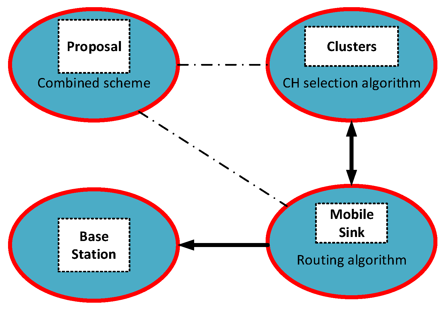
- we construct a heterogeneous WSN with mobile sink in order to minimize energy consumption and maximize the network lifetime;
- we develop a CH selection algorithm based on bacterial foraging paradigm. CHs are dynamically selected from the advanced nodes according to the proposed algorithm. These method differs from the existing studies. In this way, we obtain more shorter mobile sink trajectory sets when compared to other works;
- unlike other works, we combine the CH selection algorithm with proposed energy and transmission boundary range-aware routing algorithm developing the mathematically formulations;
- the energy model of our study consists of listening channel and sensing energy consumptions consideration as well as transmission and receiving costs; and,
- in this paper, we have implemented comprehensive simulation analyzes by measuring lots of performance metrics, including average advanced energy usage that we introduced.
2. Literature Survey
3. Preliminaries
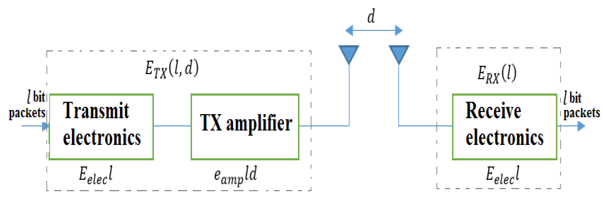
3.1. Energy Model
- Energy consumed during the transmission process.
- Energy consumed during the receiving process.
- Energy consumed for sensing.
- Energy consumed for listening during the TDMA (Time Division Multiple Access)-cycle.
3.1.1. Analysis of the Transmission and Receiving Energy Consumption Model
3.1.2. Analysis of the Listening and Sensing Energy Consumption Model
3.2. Network Model
4. Proposed CH Selection Algorithm Based Bacterial Foraging Paradigm
4.1. Overview of the Bacterial Foraging Model
4.2. The Proposed CH Selection Algorithm
4.2.1. Vocabulary
4.2.2. the Step of Chemotaxis
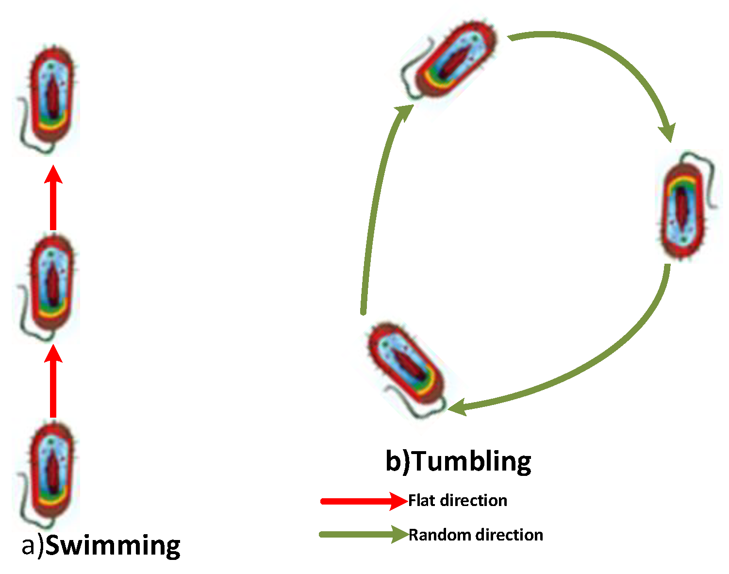
- Swimming: In every bacterial cell (BC) action, the bacteria numbered as {1,2,…, } move and the bacteria { + 1, + 2, …, } do not move. This manner is much simpler than synchronous decisions regarding swimming to simulate. Algorithm 1 shows the pseudo code of the swimming step.
- ii.
- Tumbling: In this sub step, each element produces a random vector . We use the formula that is given in Equation (11) for bacterial tumbling movement.
| Algorithm 1: An algorithm for the swimming method. |
| 1:Input: , ,,, . |
| 2:Output: New value of the after swimming movement. |
| 3: /*for computing swim length*/ |
| 4: while do /*for not exceeding the maximum number of swim steps */ |
| 5: |
| 6: if then /* a more advantageous direction*/ |
| 7: |
| 8: |
| 9: end if |
| 10: end while |
| 11: return |
| Algorithm 2: An algorithm for the chemotaxis step. |
| 1:Input: Population ( ,. |
| 2:Output: New value of the |
| 3: for Population do |
| 4: Population, ,); |
| 5: ; |
| 6: |
| 7: for do |
| 8: RandomMoveDirection=CreateMove(); |
| 9: GetMove(RandomMoveDirection,); |
| 10: if then |
| 11: ; |
| 12: else |
| 13: ; |
| 14: ; |
| 15: end if |
| 16: end for |
| 17: end for |
| 18: return |
4.2.3. The Step of Reproduction
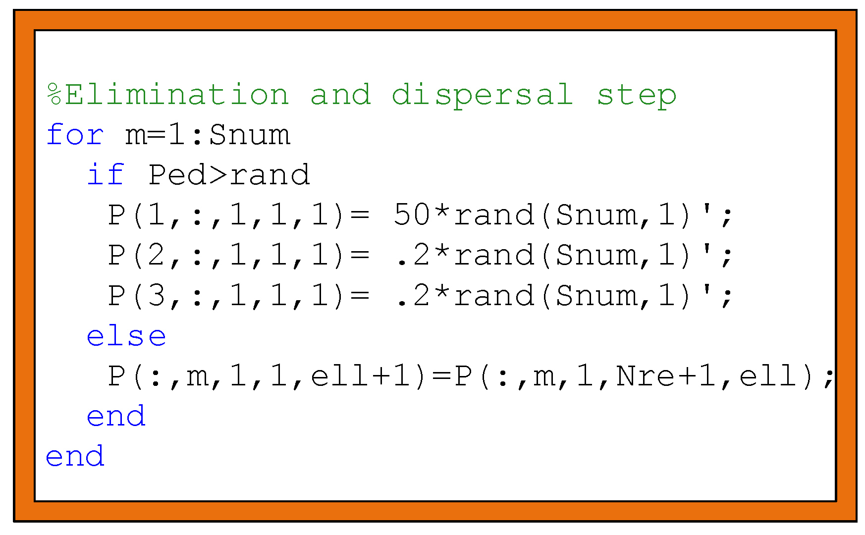
4.2.4. The Step of Elimination and Dispersal
| Algorithm 3: The proposed cluster head (CH) selection algorithm. |
| 1: Input: ,, , , ,, |
2: Output: |
| 3: Compute the and values according to Equations (14) and (15), respectively; |
| 4: Population=InitializePopulation (,); |
| 5: for =0 do |
| 6: for do |
| 7: for do |
| 8: Chemotaxis( ,); |
| 9: for Population do |
| 10: Broadcast the value as packet format defined in Figure 6. |
| 11: if then |
| 12: ; //save the set of |
| 13:else |
| 14: will be assigned to cluster with minimum |
| within transmission range ; |
| 15: end if |
| 16: end for |
| 17: end for |
| 18: OrderBCHealth(Population); |
| 19: Choosen= Choose Health (Population,; |
| 20: Population= Choosen; |
| 21: end for |
| 22: for Population do |
| 23: if then |
| 24: =CreateInRandomPosition(); |
| 25: end if |
| 26: end for |
| 27: end for |
| 28: return ; |
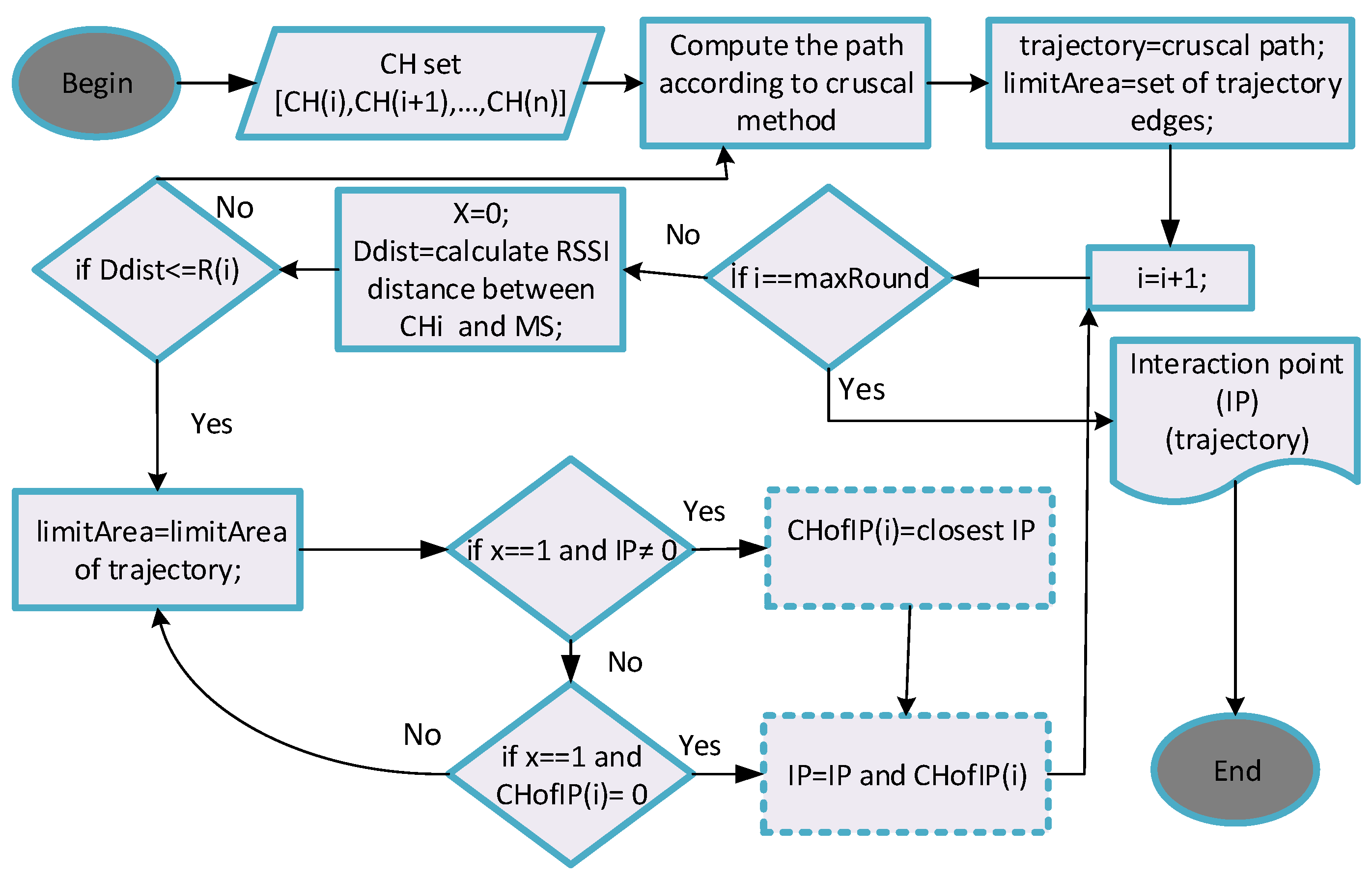
4.3. Proposed Energy-Transmission Boundary Range-Cognitive Routing Algorithm
| Algorithm 4: Proposed energy-delay and transmission aware routing algorithm. |
| 1:Input: Set of [ |
| 2:Output: trajectory of MS. |
| 3:Compute the path according to cruscal method; |
| 4:trajectory=cruscal path; |
| 5:limitArea=set of trajectory edges; |
| 6:for =1 to n do |
| 7: =0; |
| 8: =calculate RSSI distance between and MS; |
| 9: if ≤ then |
| 10: =1; |
| 11: limitArea=limitArea of trajectory; |
| 12: end if |
| 13: if =1 then |
| 14: if then |
| 15: ; |
| 16: end if |
| 17: if then |
| 18: |
| 19: end if |
| 20: end for |
5. Simulation Results
5.1. Simulation Setup
5.2. Performance Evaluation
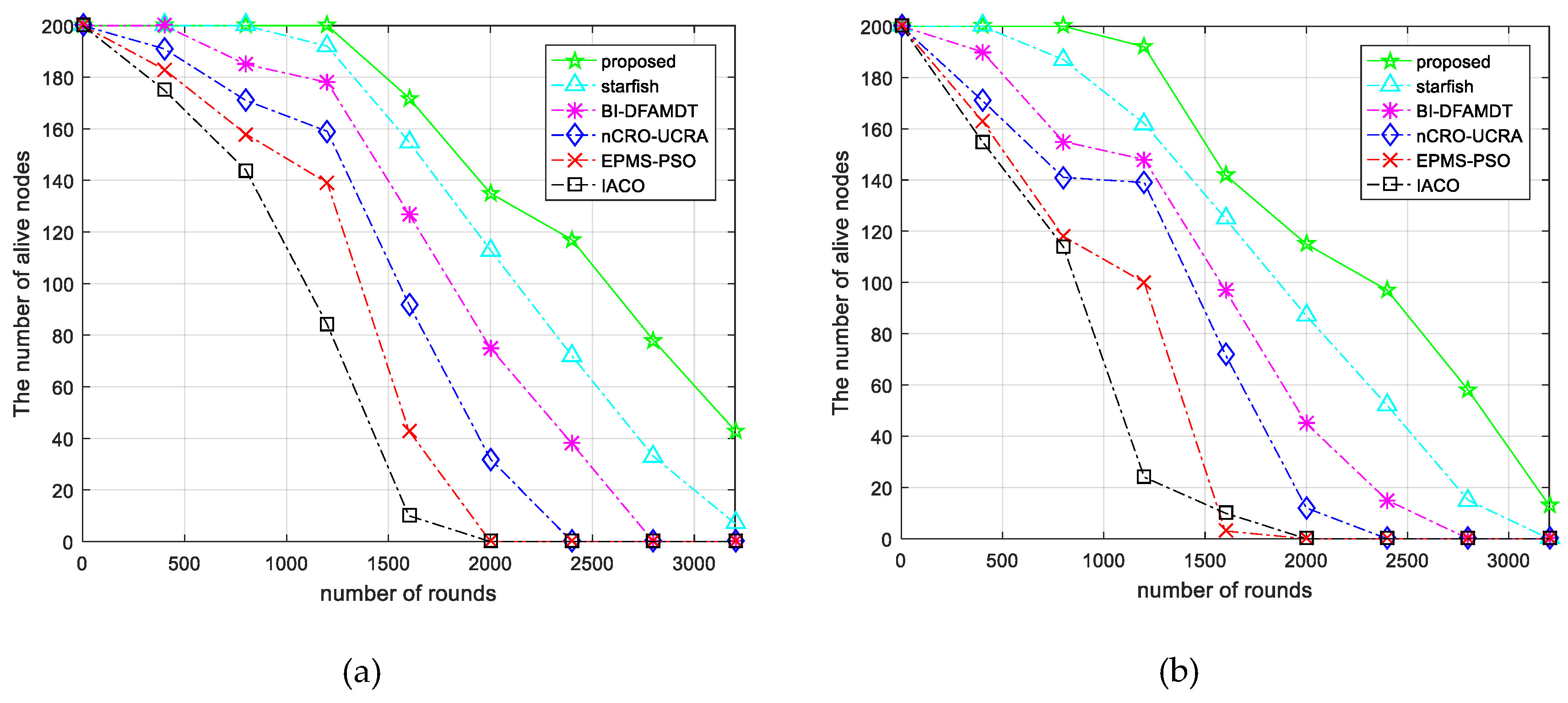
- Number of alive nodes in the network: The alive nodes metric is taking into consideration the first node’s starting to die and all the nodes’s dying. We have tested our proposed algorithm over the other protocols varying two scenarios, including scenario 1 and scenario 2 in terms of the number of alive nodes in the network. We have used 200 nodes that are distributed in the network. As seen in Figure 11a, the nodes starts to die after the 1224 th round, while using our algorithm in the scenario 1. This result validates that the proposed method outperforms the existing algorithms for longer rounds. This is because the proposed algorithm is able to utilize the network energy in a balanced manner. Additionally, as shown in Figure 11b, all of the algorithms provide less performance than before when we simulate them in scenario 2. However, our algorithm is still the best performance in comparing the other algorithms. We notice that it requires more sensor nodes deployed in the sensing area to continue for longer rounds in large-scale wireless sensor networks.
- Total remaining energy of the network: By this performance metric, the total residual energy over the lifetime of the network is calculated. We have comprehensively simulated the performance of the proposed algorithm over the other algorithms in both scenarios in terms of the remaining energy of the network versus the number of rounds.
- iii.
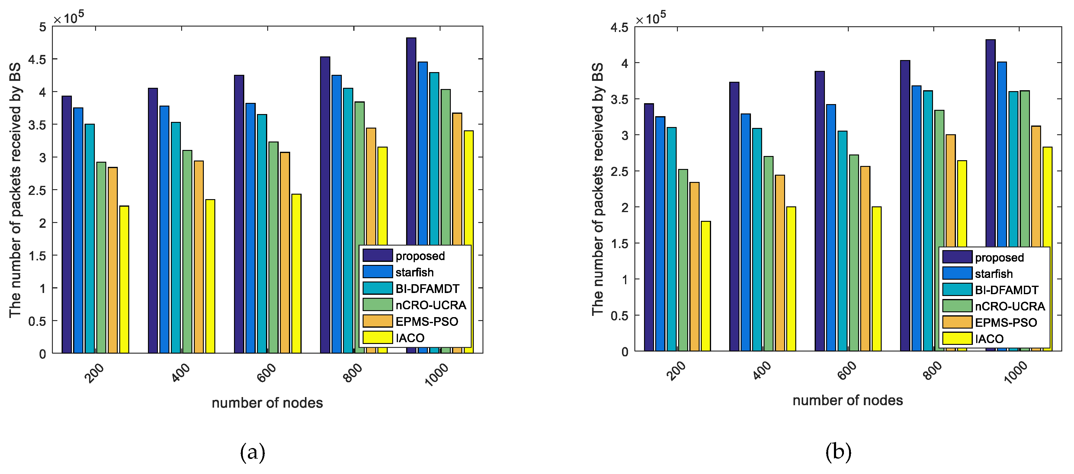
- Number of packets received by BS: By this performance metric, the total number of packets received by BS is taken into account. We have run the algorithms with respect to the number of packets received by BS varying from 200 to 1000 sensor nodes for scenario 1 and scenario 2. As seen in Figure 13a, if our proposal protocol is used in the simulations, the total number of packets that are received by BS is almost 3.9 × , 4.1 × , 4.25 × , 4.5 × , and 4.8 × for 200, 400, 600, 800, and 1000 nodes, respectively. According to Figure 13b, the total number of packets received by BS considerably diminishes because of more packet losing in the scenario 2 than another. We observe the most and least data packets obtained by the BS in the proposed method and I-ACO. This is due to the fact that our algorithm developed as combine and mobile structure, and can be delivered the packets to the destination more accurately when compared to others.
- iv.
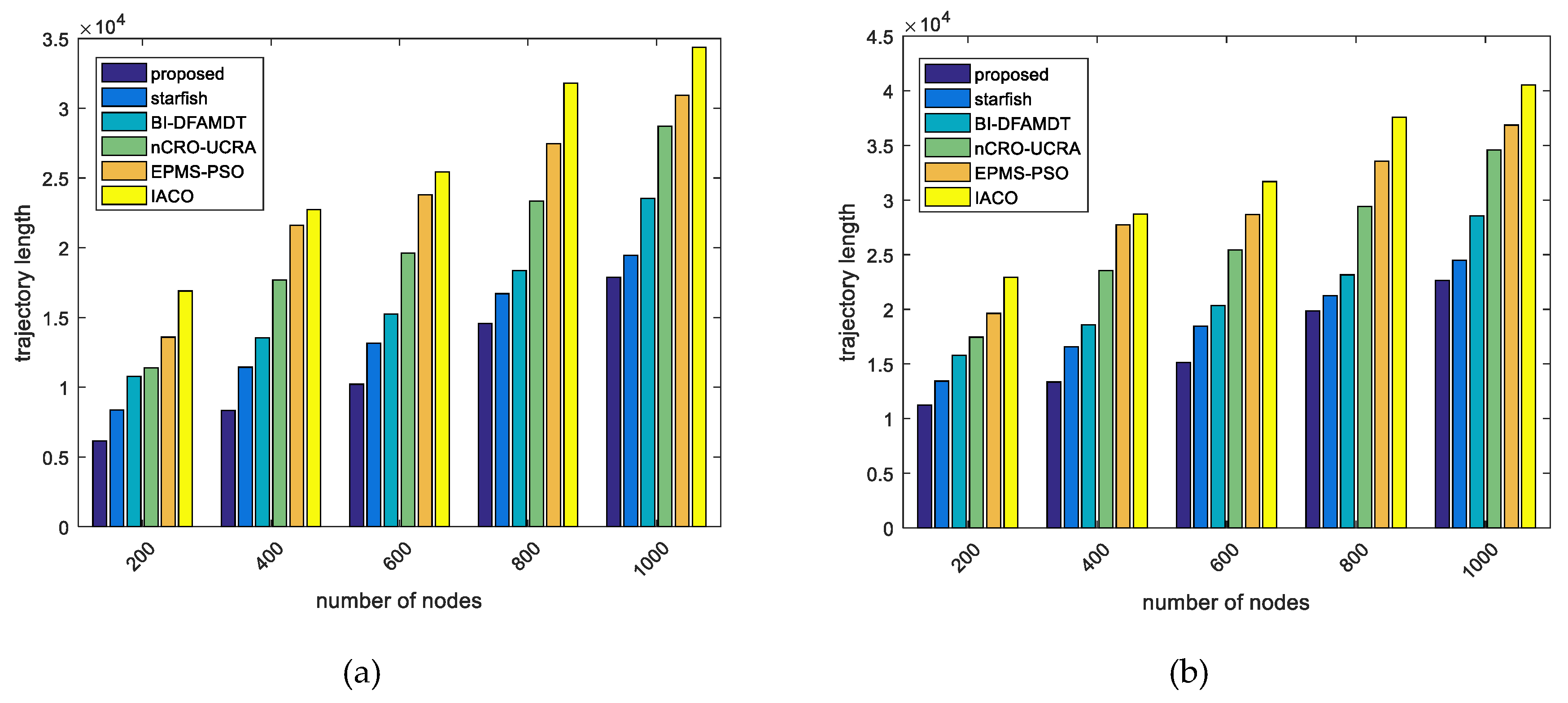
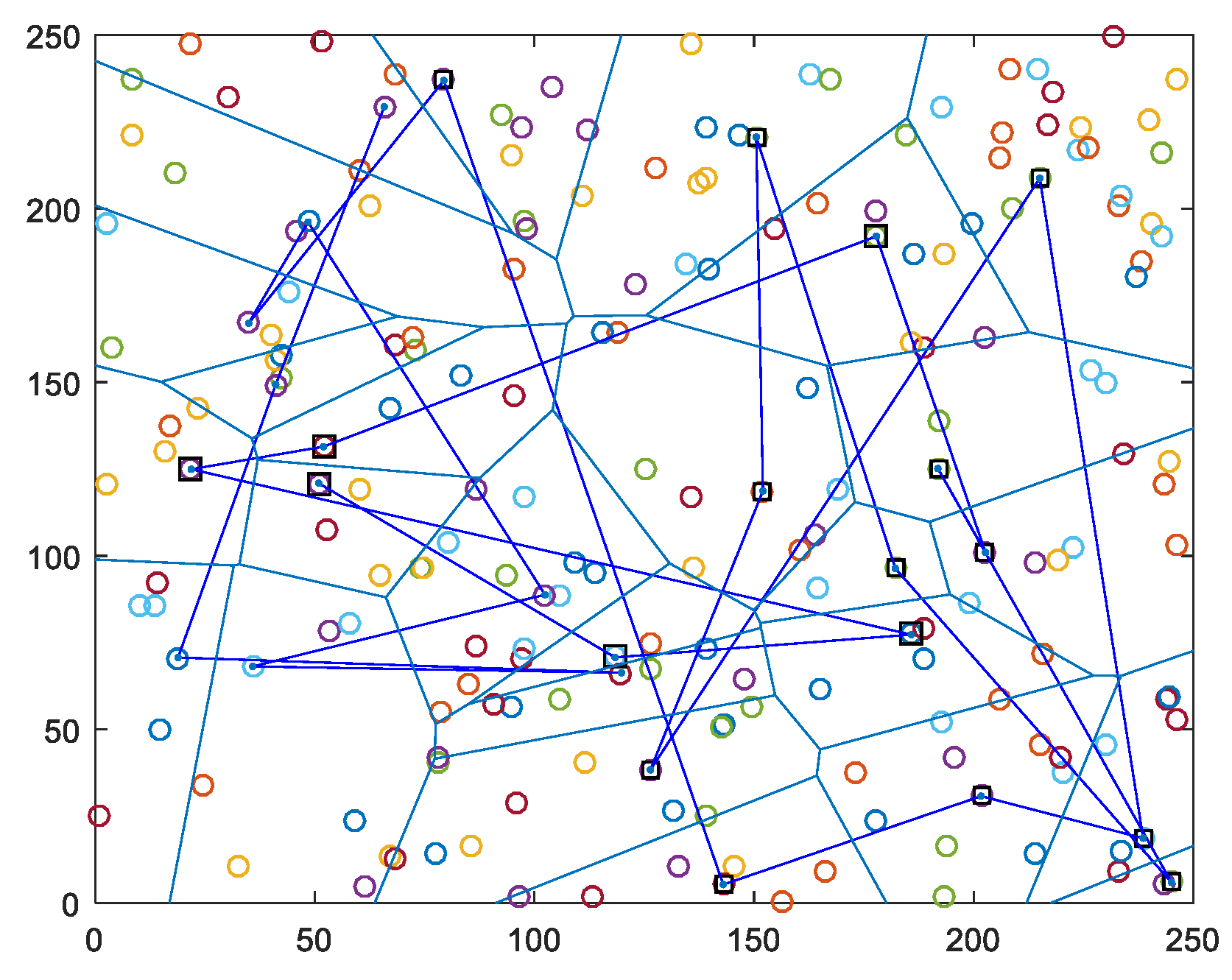
- Trajectory length travelled by MS: This is total routing path length visited by MS. We have experimented all of the algorithms according to trajectory length performance parameter varying from 200 to 1000 sensor nodes that were deployed randomly in the network.
- v.
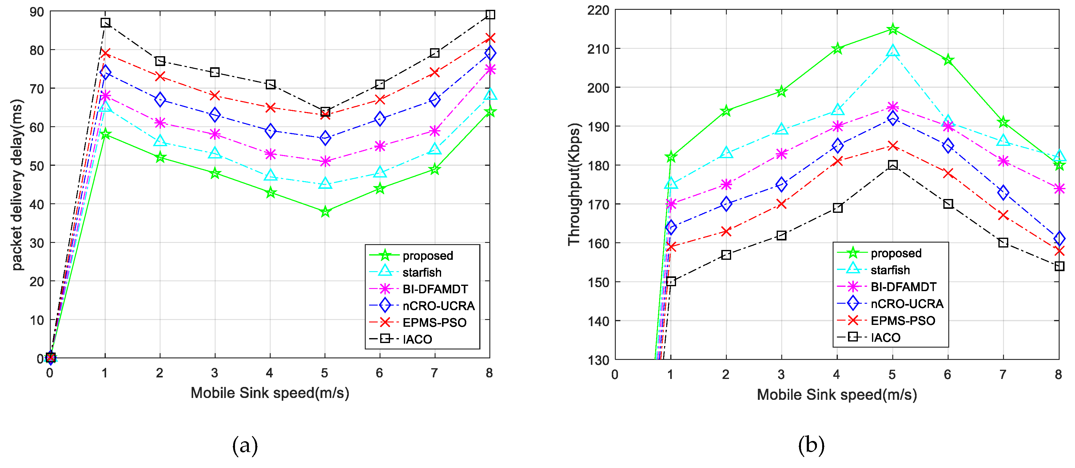
- Packet delivery delay: This is the latency time to deliver data from the source node to the destination node (MS). The lower value means it gives better performance. As shown in Figure 16a, Packet delivery delay decreases in all of the algorithms as the mobile sink speed is about 5 m/s. It occurs, owing to the fact that the sink motility significantly minimizes the hop number and the distance of the sent data packets to the BS. However, higher mobile sink speed leads to obtaining sink possition information. We note that the proposed scheme demonstrates the lowest packet delivery delay among the algorithms compared, as it is able to discover the shortest trajectories.
- vi.
- Throughput: This performance criterion means how accurately the data is transmitted and how accurate the data is delivered from the first bit to the last bit. We have assessed the performances of the algorithm for varying mobile sink speeds from 1 m/s to 8 m/s. The results clearly show that throughput increases with the mobile sink speed up to 5 m/s for all algorithms, as plotted in Figure 16b. However, once the speed of the mobile sink increases more quickly, the throughput value decreases, owing to the fact that MS trajectories change rapidly. The throughput for our proposed algorithm is better than those of other protocols due to the best MS communication with CHs. In this way, MS could gather more accurate data from CHs and deliver it to the BS.
- vii.
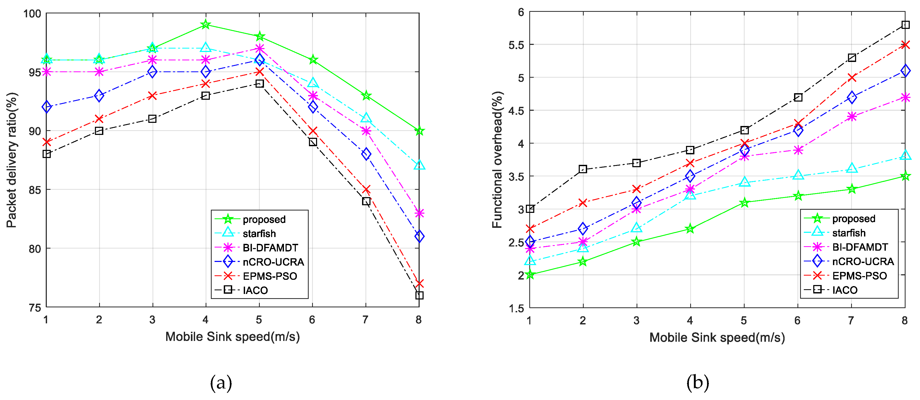
- Packet delivery rate: This metric is the ratio of the number of received packets at the mobile sink to the send packets by source nodes. The higher value means that it gives better performance. As illustrated in Figure 17a, the proposed protocol demonstrates the higher packet delivery ratio of 99% with increasing sink speed, especially between 4 and 5 m/s, and this ratio sharply decreases after the speed of the mobile sink increases. This performance validates the benefits of using appropriate mobile sink speed in the network.
- viii.
- Functional overhead: By this performance metric, the number of data packets that is received by the MS is computed. As shown in Figure 17b, the functional overhead of the proposed system is the lowest among the other presented algorithms. This originated because of the clustering of the network and routing to BS with best CH selection in the clusters. This protocol guarantees the single hop communication with BS. On the other hand, it can be observed that functional overhead increases fairly while mobile sink speed increases.
- ix.
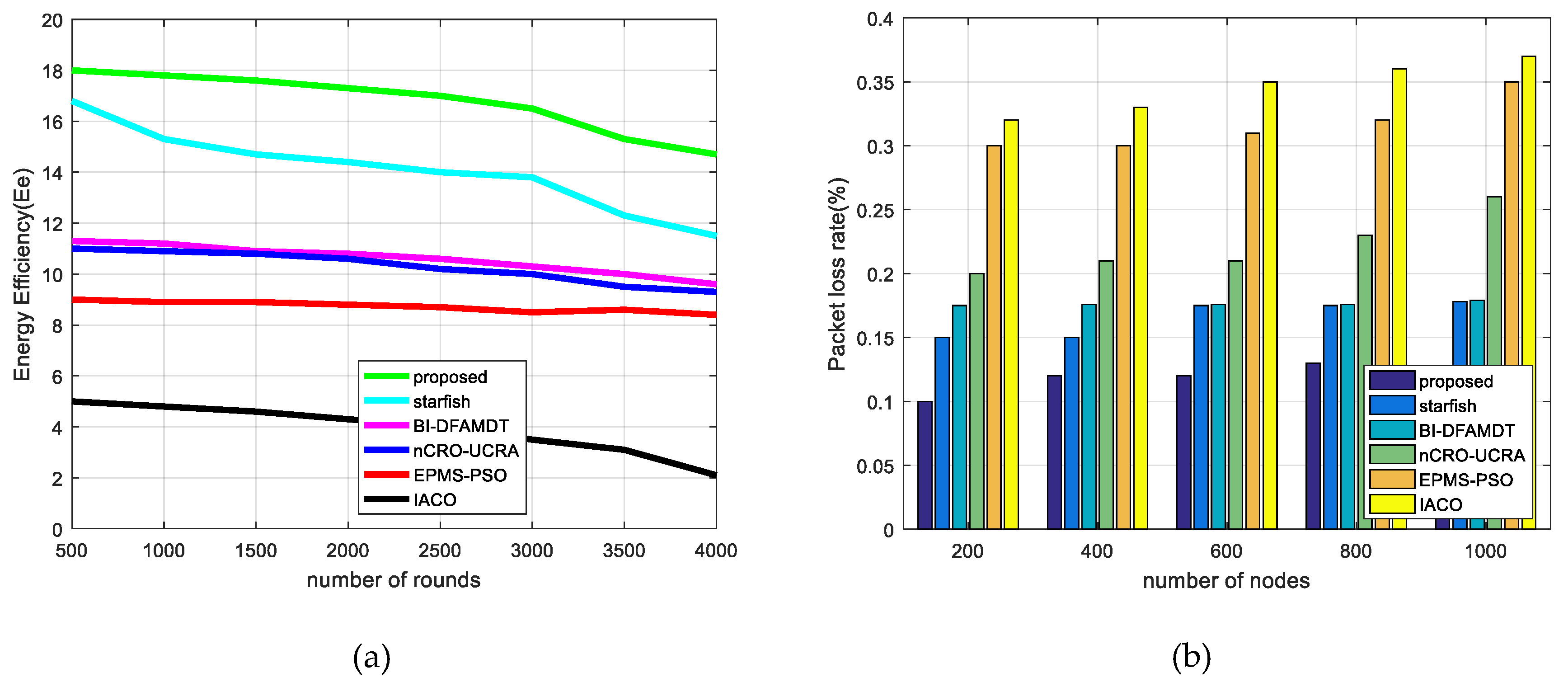
- Energy efficiency (: This metric is used for a performance measurement that observes the network life time. It is calculated via assessing the ratio of the total number of transmitted packets to the BS and the overall network’s energy consumption during the simulation rounds. The formula of energy efficiency ratio is presented in Equation (17). We have executed the presented algorithms by simulations according to the energy efficiency during the round iterations. Figure 18a demonstrates that the performance results of the IACO, PSO, nCRO-UCRA, BI-DFAMDT, starfish algorithm, and our proposal scheme are given as the ordered level from the least to most energy efficient level. Although it has partially disrupted after the 3100th round, it has generally demonstrated stable energy efficiency. The proposed algorithm expends less energy thanks to the balanced CH selection algorithm and energy aware routing mechanism in the heterogeneous network.
- x.
- Packet loss rate (): The goal of using this metric, calculated by a formula given in Equation (18), is informing the rate of packet losses due to the functionality of the implemented protocol. We have tested the worked algorithms in terms of packet loss rate versus the number of nodes.As seen in Figure 18b, our proposed algorithm produces the least packet loss rate among the algorithms. As the number of nodes increases in the network, the packet loss rate also increases due to the events of packet collisions and uncorrect packet deliverations.
- xi.
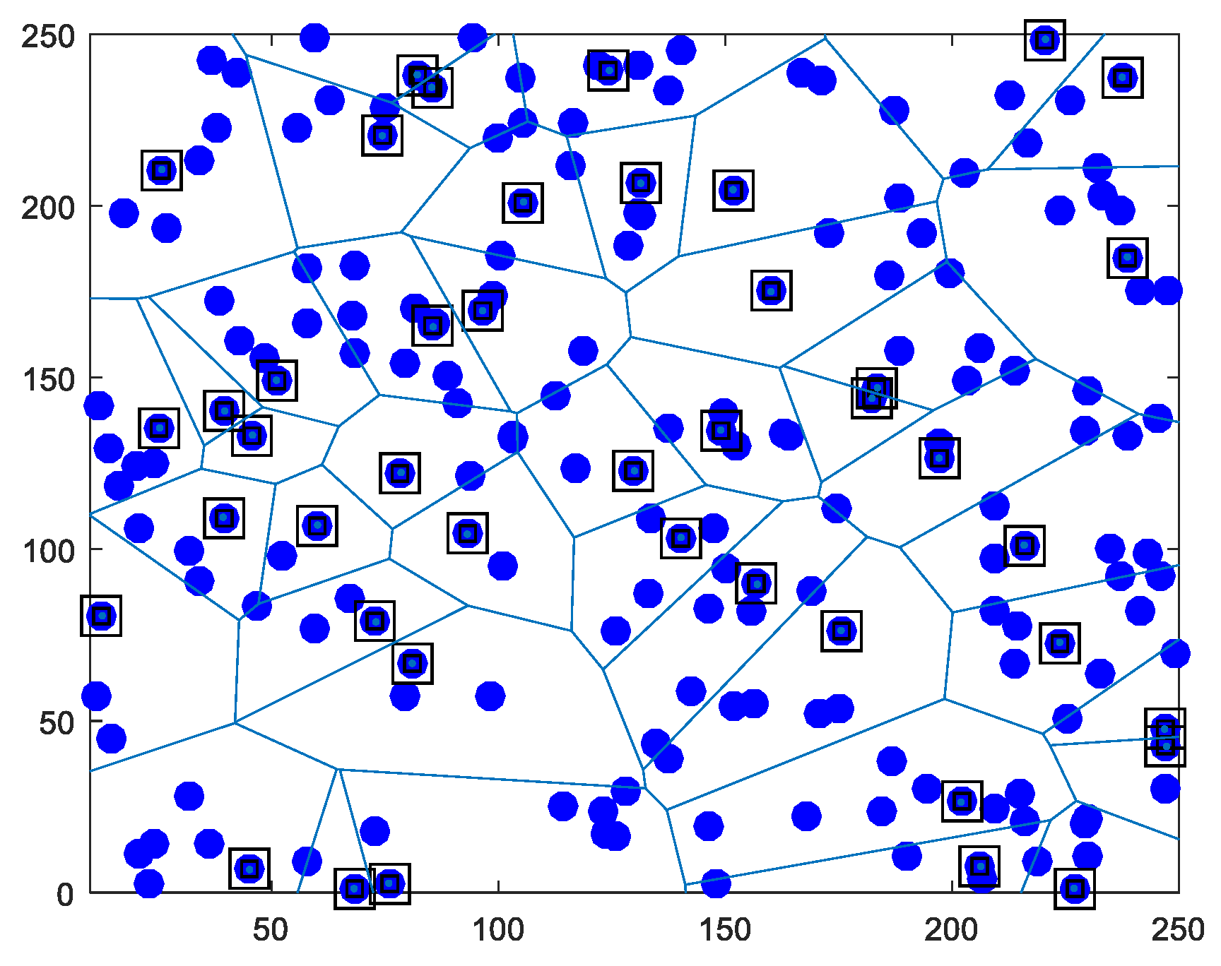
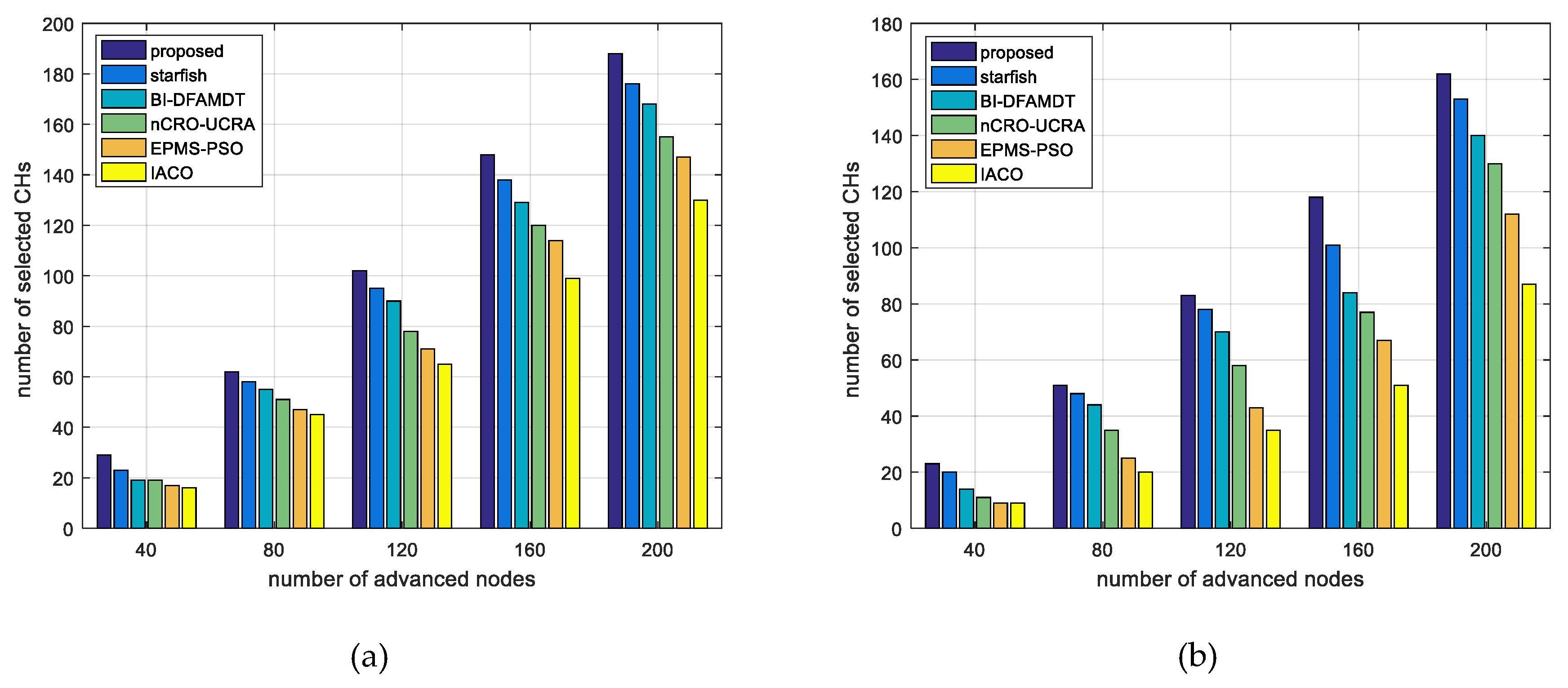
- Number of selected CHs and advanced energy usage rate (%): We also evaluate the advanced energy usage rate as the percentage in the network. We formulate this ratio with the abbreviated name , as given in Equation (19). Normally, CHs are selected from normal nodes because there is no heterogeneity in other algorithms. However, we used the other algorithms for the comparison terms to be equal. Thus, we distributed the same number of advanced nodes to the network area as our algorithm. We have calculated the number of selected CHs using the algorithms varying from 40 to 200 advanced nodes for scenario 1 (see Figure 19a) and scenario 2 (see Figure 19b). The higher this score, the more performance on behalf of the energy of the advanced nodes is proportionally used in the network. If more CH is selected than the existing advanced nodes, the energy of the advanced nodes is not wasted. As seen in Figure 19a,b, when using our proposed algorithm, the number of selected CHs is higher for both scenarios when compared to other algorithms. However, in scenario 2, the number of selected CHs decreases because of the distance factor and the uncontrolable effect of selecting CHs (see Figure 19b). Table 7 and Table 8 present the advanced energy usage results for scenario 1 and scenario 2, respectively. According to the results, it can be said that our proposal combined scheme has achieved 88.1 and 72.8 for scenario 1 and scenario 2, respectively.
6. Conclusions and Future Work
Author Contributions
Funding
Conflicts of Interest
References
- Ahmad, I.; Shah, K.; Ullah, S. Military applications using wireless sensor networks: A survey. Int. J. Eng. Sci. 2016, 6, 7039–7043. [Google Scholar]
- Abbasi, A.Z.; Islam, N.; Shaikh, Z.A. A review of wireless sensors and networks applications in agriculture. Comput. Stand. Interfaces 2014, 36, 263–270. [Google Scholar]
- Akan, O.B.; Akyildiz, I.F. Event-to-sink reliable transport in wireless sensor networks. IEEE/ACM Trans. Netw. 2005, 13, 1003–1016. [Google Scholar] [CrossRef]
- Hamidouche, R.; Aliouat, Z.; Gueroui, A.M.; Ari, A.A.A.; Louail, L. Classical and bio-inspired mobility in sensor networks for IoT applications. J. Netw. Comput. Appl. 2018, 121, 70–88. [Google Scholar] [CrossRef]
- Bozorgi, S.M.; Rostami, A.S.; Hosseinabadi, A.A.R.; Balas, V.E. A new clustering protocol for energy harvesting-wireless sensor networks. Comput. Electr. Eng. 2017, 64, 243–247. [Google Scholar] [CrossRef]
- Lee, E.; Park, S.; Yu, F.; Kim, S.H. Communication model and protocol based on multiple static sinks for supporting mobile users in wireless sensor networks. IEEE Trans. Consum. Electron. 2010, 56, 1652–1660. [Google Scholar] [CrossRef]
- Lou, W.; Kwon, Y. H-SPREAD: A hybrid multipath scheme for secure and reliable data collection in wireless sensor networks. IEEE Trans. Veh. Technol. 2006, 55, 1320–1330. [Google Scholar] [CrossRef]
- Liu, A.; Huang, M.; Zhao, M.; Wang, T. A smart high-speed backbone path construction approach for energy and delay optimization in wsns. IEEE Access 2018, 6, 13836–13854. [Google Scholar] [CrossRef]
- Avril, F.; Bernard, T.; Bui, A.; Sohier, D. Clustering and communications scheduling in WSNs using mixed integer linear programming. J. Commun. Netw. 2014, 16, 421–429. [Google Scholar] [CrossRef]
- Chen, H.; Mineno, H.; Mizuno, T. A meta-data-based data aggregation scheme in clustering wireless sensor networks. In Proceedings of the 7th International Conference on Mobile Data Management, Nara, Japan, 10–12 May 2006; p. 154. [Google Scholar]
- Arun, K.; Katiyar, V.K. Intelligent Cluster Routing: An Energy Efficient Approach for Routing in Wireless Sensor Networks. Int. J. Comput. Appl. 2015, 110, 18–22. [Google Scholar]
- Khan, M.I.; Gansterer, W.N.; Haring, G. Static vs. mobile sink: The influence of basic parameters on energy efficiency in wireless sensor networks. Comput. Commun. 2013, 36, 965–978. [Google Scholar] [CrossRef] [PubMed]
- Lin, Z.; Zhang, H.; Wang, Y.; Yao, F. Energy-efficient routing protocol on mobile sink in wireless sensor network. Adv. Mater. Res. 2013, 787, 1050–1055. [Google Scholar] [CrossRef]
- Qing, L.; Zhu, Q.; Wang, M. Design of a distributed energy-efficient clustering algorithm for heterogeneous wireless sensor network. Comput. Commun. 2006, 29, 2230–2237. [Google Scholar] [CrossRef]
- Singh, S.K.; Singh, M.P.; Singh, D.K. Routing protocols in wireless sensor networks—A survey. Int. J. Comput. Sci. Eng. Surv. 2010, 1, 63–83. [Google Scholar] [CrossRef]
- Hammoudeh, M.; Newman, R. Adaptive routing in wireless sensor networks: QoS optimization for enhanced application performance. Inf. Fusion 2015, 22, 3–15. [Google Scholar] [CrossRef]
- Hamida, E.B.; Chelius, G. A line-based data dissemination protocol for wireless sensor networks with mobile sink. In Proceedings of the 2008 IEEE International Conference on Communications, Beijing, China, 19–23 May 2008; pp. 2201–2205. [Google Scholar]
- Nur, F.N.; Sharmin, S.; Habib, M.A.; Razzaque, M.A.; Islam, M.S.A.; Ahmad, H.; Mohammad, M.; Alamri, A. Collaborative neighbor discovery in directional wireless sensor networks: Algorithm and analysis. EURASIP J. Wirel. Commun. Netw. 2017, 2017, 119. [Google Scholar] [CrossRef]
- Das, A.; Dutta, D. Data acquisition in multiple-sink sensor networks. Mob. Comput. Commun. Rev. 2005, 9, 82–85. [Google Scholar] [CrossRef]
- Salarian, H.; Chin, K.W.; Naghdy, F. An energy-efficient mobile-sink path selection strategy for wireless sensor networks. IEEE Trans. Veh. Technol. 2013, 63, 2407–2419. [Google Scholar] [CrossRef]
- Li, J.; Dang, J.; Bu, F.; Wang, J. Analysis and improvement of the bacterial foraging optimization algorithm. J. Comput. Sci. Eng. 2014, 8, 1–10. [Google Scholar] [CrossRef]
- Ketel, M.; Dogan, N.S.; Homaifar, A. Distributed sensor networks based on mobile agents paradigm. In Proceedings of the 37th Southeastern Symposium on System Theory (SSST’05), Tuskegee, AL, USA, 20–22 March 2005; pp. 411–414. [Google Scholar]
- Sharma, A.; Thakur, J. An energy efficient network life time enhancement proposed clustering algorithm for Wireless Sensor Networks. Int. J. Enhanc. Res. Manag. Comput. Appl. 2014, 2, 1–4. [Google Scholar]
- Han, S.W.; Jeong, I.S.; Kang, S.H. Low latency and energy efficient routing tree for wireless sensor networks with multiple mobile sinks. J. Netw. Comput. Appl. 2013, 36, 156–166. [Google Scholar] [CrossRef]
- Nanda, S.J.; Panda, G. A survey on nature inspired metaheuristic algorithms for partitional clustering. Swarm Evol. Comput. 2014, 16, 1–18. [Google Scholar] [CrossRef]
- Ari, A.A.A.; Yenke, B.O.; Labraoui, N.; Damakoa, I.; Gueroui, A. A power efficient cluster-based routing algorithm for wireless sensor networks: Honeybees swarm intelligence based approach. J. Netw. Comput. Appl. 2016, 69, 77–99. [Google Scholar] [CrossRef]
- Saleem, M.; DiCaro, G.A.; Farooq, M. Swarm intelligence based routing protocol for wireless sensor networks: Survey and future directions. Inf. Sci. 2011, 181, 4597–4624. [Google Scholar] [CrossRef]
- Yang, J.; Xu, M.; Zhao, W.; Xu, B. A multi path routing protocol based on clustering and ant colony optimization for wireless sensor networks. Sensors 2010, 10, 4521–4540. [Google Scholar] [CrossRef] [PubMed]
- Rostami, A.; Mottar, M.H. Wireless sensor networks clustering using particles swarm optimization for reducing energy consumption. Int. J. Manag. Inf. Technol. 2014, 6, 1–15. [Google Scholar] [CrossRef]
- Gambhir, A.; Payal, A.; Arya, R. Performance analysis of artificial bee colony optimization based clustering protocol in various scenarios of WSN. Int. J. Manag. Inf. Technol. 2018, 132, 183–188. [Google Scholar] [CrossRef]
- Yogarajan, G.; Revathi, T. Nature inspired discrete firefly algorithm for optimal mobile data gathering in wireless sensor networks. Wirel. Netw. 2017, 24, 2993–3007. [Google Scholar] [CrossRef]
- Mua’zu, M.B.; Salawudeen, A.T.; Sikiru, T.H.; Abdu, A.; Mohammad, A. Weighted artificial fish swarm algorithm with adaptive behaviour based linear controller design for nonlinear inverted pendulum. J. Eng. Res. 2015, 20, 1–12. [Google Scholar]
- Habib, A.; Saha, S.; Razzaque, A.; Rashid, M.; Fortino, G.; Hassan, M.M. Starfish routing for sensor networks with mobile sink. J. Netw. Comput. Appl. 2018, 123, 11–22. [Google Scholar] [CrossRef]
- Iftikhar, M.S.; Fraz, M.R. A survey on application of swarm intelligence in network security. Trans. Mach. Learn. Artif. Intell. 2013, 1, 1–15. [Google Scholar]
- Ari, A.A.A.; Gueroui, A.; Labraoui, N.; Yenke, B.O. Concepts and evolution of research in the field of wireless sensor networks. Int. J. Comput. Netw. Commun. 2015, 7, 81–98. [Google Scholar]
- Yang, J.; Ding, R.; Zhang, Y.; Cang, M. An improved ant colony optimization (I-ACO) method for the quasi travelling salesman problem (quasi-TSP). Int. J. Geogr. Sci. Inf. 2015, 29, 1–18. [Google Scholar] [CrossRef]
- Wang, J.; Cao, Y.; Li, B.; Kim, H.J.; Lee, S. Particle swarm optimization based clustering algorithm with mobile sink for WSNs. Future Gener. Syst. 2017, 76, 452–457. [Google Scholar] [CrossRef]
- Rao, P.C.S.; Banka, H. Novel chemical reaction optimization based unequal clustering and routing algorithms for wireless sensor networks. Wirel. Netw. 2017, 23, 759–778. [Google Scholar] [CrossRef]
- Heinzelman, W.R.; Chandrakasan, A.; Balakrishnan, H. Energy-efficient communication protocol for wireless microsensor networks. In Proceedings of the 33rd Annual Hawaii International Conference on System Sciences, Maui, HI, USA, 7 January 2000; pp. 10–20. [Google Scholar]
- Heinzelman, W.B.; Chandrakasan, A.P.; Balakrishnan, H. An application specific protocol architecture for wireless microsensor networks. IEEE Trans. Wirel. Commun. 2002, 1, 660–670. [Google Scholar] [CrossRef]
- Smaragdakis, G.; Matta, I.; Bestavros, A. SEP: A Stable Election Protocol for Clustered Heterogeneous Wireless Sensor Network. In Proceedings of the Second International Workshop on Sensor and Actor Network Protocols and Applications (SANPA), Boston, MA, USA, 31 May 2004; pp. 1–11. [Google Scholar]
- Ma, M.; Yang, Y. SenCar: An energy-efficient data gathering mechanism for large-scale multihop sensor networks. IEEE Trans. Parallel Distrib. Syst. 2007, 18, 1476–1488. [Google Scholar] [CrossRef]
- Chen, J.; Sayed, A.H. Bio-inspired cooperative optimization with application to bacterial motility. In Proceedings of the 2011 IEEE International Conference on Acoustics, Speech and Signal Processing (ICASSP), Prague, Czech Republic, 22–27 May 2011; pp. 5788–5791. [Google Scholar]
- Dhiman, V. Bio inspired hybrid routing protocol for wireless sensor networks. Int. J. Adv. Res. Eng. Technol. 2013, 1, 33–36. [Google Scholar]
- Lindsey, S.; Raghavenda, C.S. PEGASIS: Power efficient gathering in sensor information systems. In Proceedings of the IEEE Aerospace Conference, Big Sky, MT, USA, 9–16 March 2002. [Google Scholar]
- Ahmet, G.; Zou, J.; Fareed, M.M.S.; Zeeshan, M. Sleep-awake energy efficient distributed clustering algorithm for wireless sensor networks. Comput. Electr. Eng. 2015, 56, 385–398. [Google Scholar] [CrossRef]
- Vançin, S.; Erdem, E. Performance analysis of the energy efficient clustering models in wireless sensor networks. In Proceedings of the 2017 24th IEEE International Conference on Electronics, Circuits and Systems (ICECS), Batumi, Georgia, 5–8 December 2017; pp. 247–251. [Google Scholar]
- Alsaafin, A.; Khedr, A.M.; Aghbari, Z.A. Distributed trajectory design for data gathering using mobile sink in wireless sensor networks. AEU Int. J. Electron. Commun. 2018, 96, 1–12. [Google Scholar] [CrossRef]
- Elhabyan, R.; Shi, W.; Hilaire, M. A Pareto optimization-based approach to clustering and routing in Wireless Sensor Networks. J. Netw. Comput. Appl. 2018, 114, 57–69. [Google Scholar] [CrossRef]
- Vançin, S.; Erdem, E. Threshold Balanced Sampled DEEC Model for Heterogeneous Wireless Sensor Network. Wirel. Commun. Mob. Comput. 2018, 2018, 1–12. [Google Scholar] [CrossRef]
- Annu, S.; Chaudhary, J. A review of BFOA applications to WSN. Int. J. Adv. Found. Res. Comput. 2015, 2, 1–15. [Google Scholar]
- Niu, B.; Wang, J.; Wang, H. Bacterial-inspired algorithms for solving constrained optimization problems. J. Neurocomput. 2015, 148, 54–62. [Google Scholar] [CrossRef]
- Dasgupta, S.; Das, S.; Abraham, A.; Biswas, A. Adaptive computational chemotaxis in bacterial foraging optimization: an analysis. IEEE Trans. Evol. Comput. 2009, 13, 919–941. [Google Scholar] [CrossRef]
- Supriyono, H.; Tokhi, M. Adaptation schemes of chemotactic step size of bacterial foraging algorithm for faster convergence. J. Artif. Intell. 2011, 4, 207–219. [Google Scholar] [CrossRef][Green Version]
- Liu, X. A survey on clustering routing protocols in wireless sensor networks. Sensors 2012, 12, 11113–11153. [Google Scholar] [CrossRef]
- Nasir, A.; Tokhi, M.O.; Ghani, N.A. Novel adaptive bacterial foraging algorithms for global optimisation with application to modelling of a TRS. Expert Syst. Appl. 2015, 42, 1513–1530. [Google Scholar] [CrossRef]
- Qiao, L.; Lingguo, C.; Baihai, Z.; Zhun, F. A low energy intelligent clustering protocol for wireless sensor networks. In Proceedings of the 2010 IEEE International Conference on Industrial Technology, Vina del Mar, Chile, 14–17 March 2010. [Google Scholar]
- Rostami, A.S.; Badkoobe, M.; Mohanna, F.; Hosseinabadi, A.A.R.; Sangaiah, A.K. Survey on clustering in heterogeneous and homogeneous wireless sensor networks. J. Supercomput. 2018, 74, 277–323. [Google Scholar]


| Bacteria Foraging Inspiration | WSN |
|---|---|
| Bacteria | Sensor nodes |
| Food density | Objective function |
| The density of nutrients in the region is not known by bacteria. | The nodes do not know the cost function in advance. |
| Bacteria can detect the density of food at their location. | The nodes can only detect changes in the values of the cost function. |
| Bacteria have a limited detection ability (which determines the local error signal) that they cannot assess the intensity, they are only aware of the sign. | When moving nodes, they are aware that only the cost function is increasing or decreasing. |
| When the nutrient density increases, the bacteria will work in this direction. Otherwise, it is affected by confusion and the bacteria performs tumble movement. | An i node follows the direction of its neighbors in the right direction. Otherwise, if none of the neighbors (including i) are in the correct direction, then the node i will change direction. |
| Notation Symbols | Notation Descriptions |
|---|---|
| Problem space | |
| Random direction vector with the same number of dimensions. | |
| The number of bacterial cells that represents sensor node in our algorithm. | |
| Initial energy of a sensor node | |
| Maximum sensor node load | |
| Remaining energy of a sensor node | |
| Load of a sensor node | |
| Node degree of a CH | |
| Euclidean distance between a sensor node and an CH within its range | |
| Transmission range of a sensor node | |
| Used for trade-off between residual energy and node load | |
| Used for trade-off between load distribution and energy consumption | |
| Using for control the number of CHs | |
| Neighbors of a sensor node that are within its transmission range | |
| The number of chemotaxis steps. | |
| The number of swim steps for a given bacterial cell | |
| The number of dimensions on a given bacterial cells position vector. | |
| The number of reproduction steps. | |
| The number of elimination-dispersal steps. | |
| Possibility of elimination and dispersal of a bacterial cell. | |
| Population | Bacterial population |
| Attraction coefficient 1 | |
| Attraction coefficient 2 | |
| The height of the repellant effect (magnitude of its effect) | |
| Measuring of the width of the bacterial repellant effect |
| Segment | Description |
|---|---|
| id | Unique definition given by a node |
| node(i)Id | source node id |
| CHiD | CH destination id |
| Eremain | Remaining energy of a sensor node |
| Emax | Maximum energy of sensor node |
| Lnode | Load of a sensor node |
| Lmax | Maximum oad of sensor node |
| DATA | Transferred data |
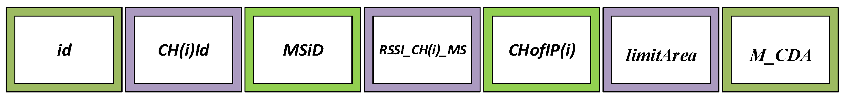
| Segment | Description |
|---|---|
| id | Unique definition given by a CH node |
| CH(i)Id | source CH node id |
| MSiD | MS destination id |
| RSSI_CH(i)_MS | RSSI distance between and MS |
| CHofIP(i) | CH intersection point |
| limitArea | Fields assigned by trajectory edges |
| M_CDA | Collected and aggregated data by CH |
| Parameters | Value |
|---|---|
| Network size | 250 × 250 and 500 × 500 |
| Number of sensor nodes | 200 to 1000 |
| Number of advanced nodes | 40–200 |
| Initial energy of normal nodes | 1 J |
| Initial energy of advanced nodes | 2 J |
| Data packet size ( | 5000 bits |
| Transmission range () | 60 m |
| Sensor node deployment | Uniformly random |
| Base station (BS) position | (0,0) |
| Mobile sink speed | 1 m/s to 8 m/s |
| 70 m | |
| 4000 bits | |
| 0.5 | |
| 2500 | |
| 50 | |
| 50 | |
| Simulation time ( | 0.5 h |
| Parameters | Value | Parameters | Value |
|---|---|---|---|
| 2 | 2 | ||
| 50–100 | 0.2 | ||
| 0.1 | 0.1 | ||
| 4 | 0.2 | ||
| 2 J | 0.1 | ||
| 5 | 10 | ||
| 4 | 50–80 m | ||
| 50 | 0.6 | ||
| 4 | 0.4 |
| The Number of Total Advanced Nodes | The Number of Selected CHs | |||||
|---|---|---|---|---|---|---|
| Proposed | Starfish | BI-DFAMDT | nCRO-UCRA | EPMS-PSO | IACO | |
| 40 | 29 | 23 | 19 | 19 | 17 | 16 |
| 80 | 62 | 58 | 55 | 51 | 47 | 45 |
| 120 | 102 | 95 | 90 | 78 | 71 | 65 |
| 160 | 148 | 138 | 129 | 120 | 114 | 99 |
| 200 | 188 | 176 | 168 | 155 | 147 | 130 |
| Total | 529 | 490 | 461 | 423 | 396 | 355 |
| (%) | 88.1 | 81.6 | 76.8 | 70.5 | 66.0 | 59.1 |
| The Number of Total Advanced Nodes | The Number of Selected CHs | |||||
|---|---|---|---|---|---|---|
| Proposed | Starfish | BI-DFAMDT | nCRO-UCRA | EPMS-PSO | IACO | |
| 40 | 23 | 20 | 14 | 11 | 9 | 9 |
| 80 | 51 | 48 | 44 | 35 | 25 | 20 |
| 120 | 83 | 78 | 70 | 58 | 43 | 35 |
| 160 | 118 | 101 | 84 | 77 | 67 | 51 |
| 200 | 162 | 153 | 140 | 130 | 112 | 87 |
| Total | 437 | 400 | 352 | 311 | 256 | 202 |
| (%) | 72.8 | 66.6 | 58.6 | 51.8 | 42.6 | 33.6 |
© 2019 by the authors. Licensee MDPI, Basel, Switzerland. This article is an open access article distributed under the terms and conditions of the Creative Commons Attribution (CC BY) license (http://creativecommons.org/licenses/by/4.0/).
Share and Cite
Yalçın, S.; Erdem, E. Bacteria Interactive Cost and Balanced-Compromised Approach to Clustering and Transmission Boundary-Range Cognitive Routing In Mobile Heterogeneous Wireless Sensor Networks. Sensors 2019, 19, 867. https://doi.org/10.3390/s19040867
Yalçın S, Erdem E. Bacteria Interactive Cost and Balanced-Compromised Approach to Clustering and Transmission Boundary-Range Cognitive Routing In Mobile Heterogeneous Wireless Sensor Networks. Sensors. 2019; 19(4):867. https://doi.org/10.3390/s19040867
Chicago/Turabian StyleYalçın, Sercan, and Ebubekir Erdem. 2019. "Bacteria Interactive Cost and Balanced-Compromised Approach to Clustering and Transmission Boundary-Range Cognitive Routing In Mobile Heterogeneous Wireless Sensor Networks" Sensors 19, no. 4: 867. https://doi.org/10.3390/s19040867
APA StyleYalçın, S., & Erdem, E. (2019). Bacteria Interactive Cost and Balanced-Compromised Approach to Clustering and Transmission Boundary-Range Cognitive Routing In Mobile Heterogeneous Wireless Sensor Networks. Sensors, 19(4), 867. https://doi.org/10.3390/s19040867