ECG Noise Cancellation Based on Grey Spectral Noise Estimation


Abstract
:1. Introduction
2. The ECG Signal, EMD and EEMD
2.1. ECG Signal
2.2. The EMD Algorithm
- Step 1.
- Find the local maxima and minima in .
- Step 2.
- Obtain the upper envelope by the local maxima and the lower envelope by local minima, respectively.
- Step 3.
- Calculate the average of the upper and lower envelops, .
- Step 4.
- Find the difference signal .
- Step 5.
- Check if is a zero-average process. If yes, then stop and treat as the first-order IMF (IMF 1), denoted as ; otherwise, replace with and go back to Step 1.
- Step 6.
- Calculate the residual signal .
- Step 7.
- Replace with and repeat Step 1 to Step 6 to find the second-order IMF (IMF 2), i.e., .
- Step 8.
- Repeat Step 1 to Step 7 till is obtained where is the total number of IMFs.
2.3. The EEMD Algorithm
- Step 1.
- Add a white noise sequence into the target signal , i.e., . In this study, noise with is used which will be verified in Section 5.1.
- Step 2.
- Apply the EMD algorithm to decompose , as described in Section 2.2.
- Step 3.
- Repeat Steps 1 and 2 until the predefined number of trials, , is reached. Each trial uses the same noise power level. Then a set of IMF components is obtained where is the iteration number and is the order of IMFs.
- Step 4.
- Calculate the ensemble average of as followswhere is the total number of trials.
3. Application of GSNE to ECG Noise Cancellation
3.1. GM(1,1) Model
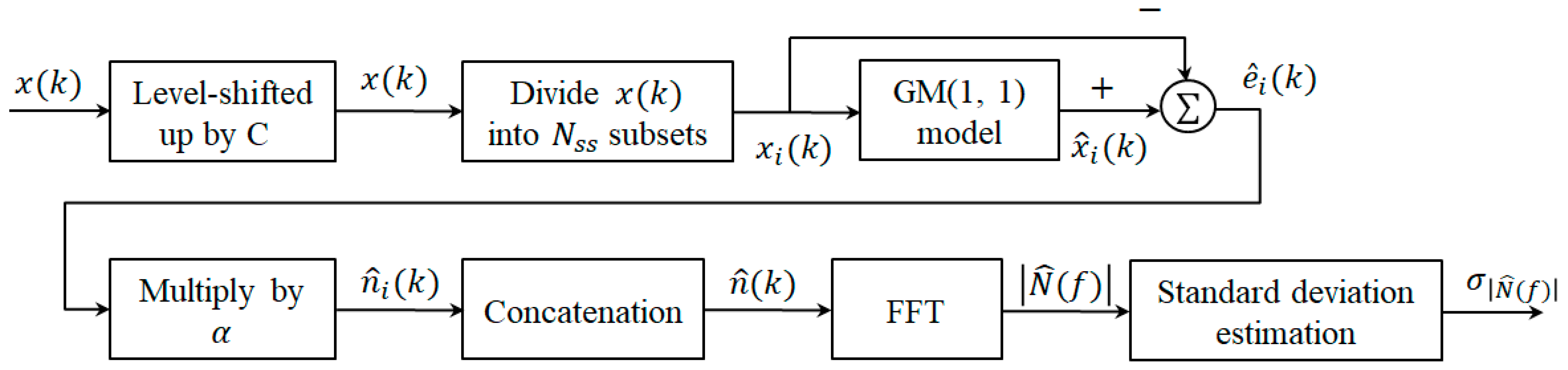
3.2. Grey Spectral Noise Estimation
- Step 1.
- Level up by a constant , i.e., such that the condition is met.
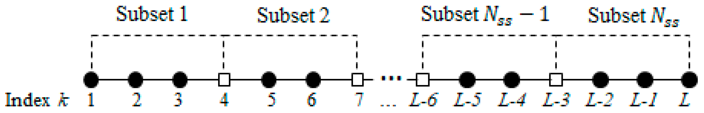
- Step 2.
- Divide into subsets as , for , where K is the number of data used in GM(1,1) model. Figure 2 indicates how is divided into subsets with K = 4 where the square refers to the overlapped sample.
- Step 3.
- For each subset , obtain the estimate of , , by the GM(1,1) model described in Section 3.1. Then, is considered as the estimate of , , that is, . Finally, calculate the estimation error of GM(1,1) model as .
- Step 4.
- Since the additive noise is not equal but related to the estimation error . Consequently, is estimated as where is the user-defined scaling factor and determined by experiences.
- Step 5.
- Apply Fast Fourier Transform (FFT) on , i.e., and find the magnitude of , where is used.
- Step 6.
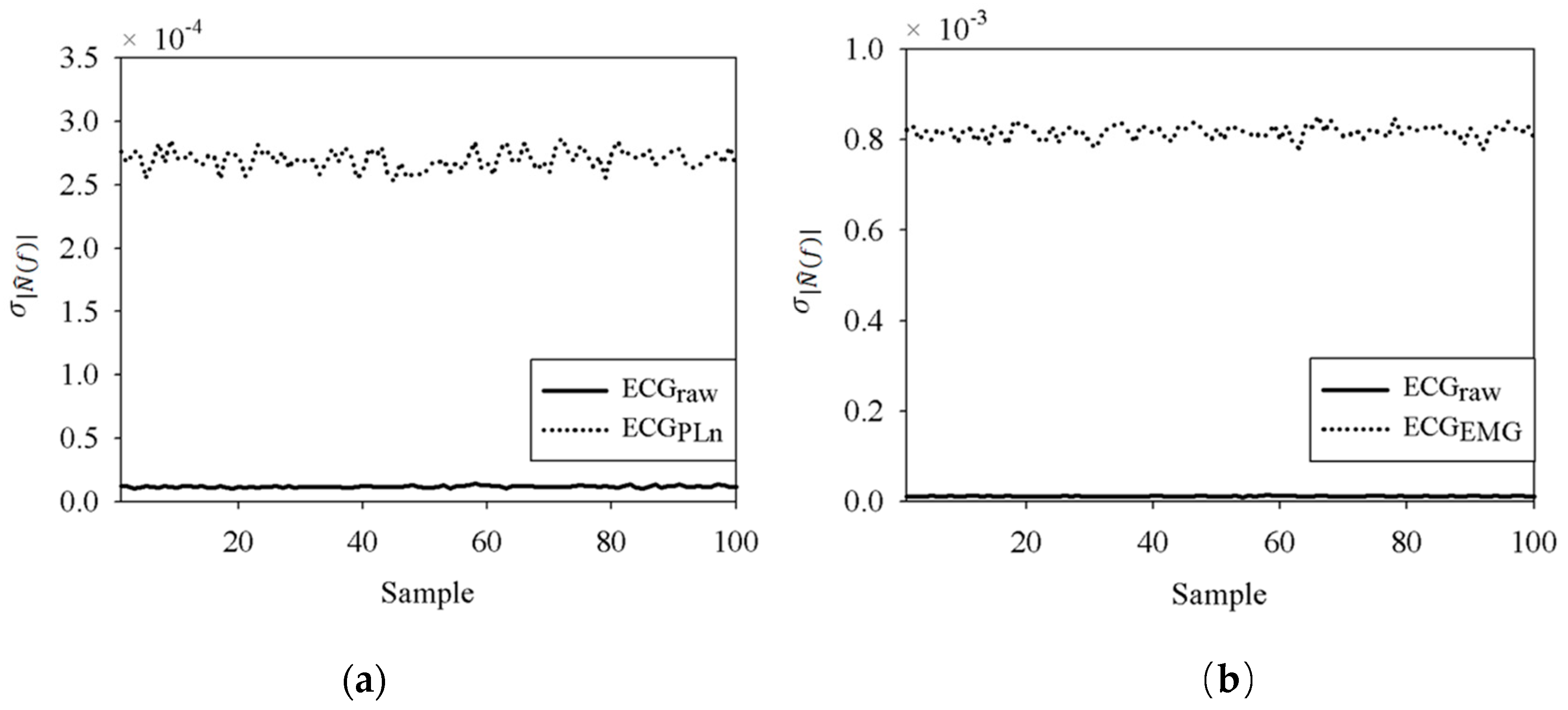
- Calculate the standard deviation of , , as an indicator of noise energy.
3.3. Noisy IMF Determination by the GSNE
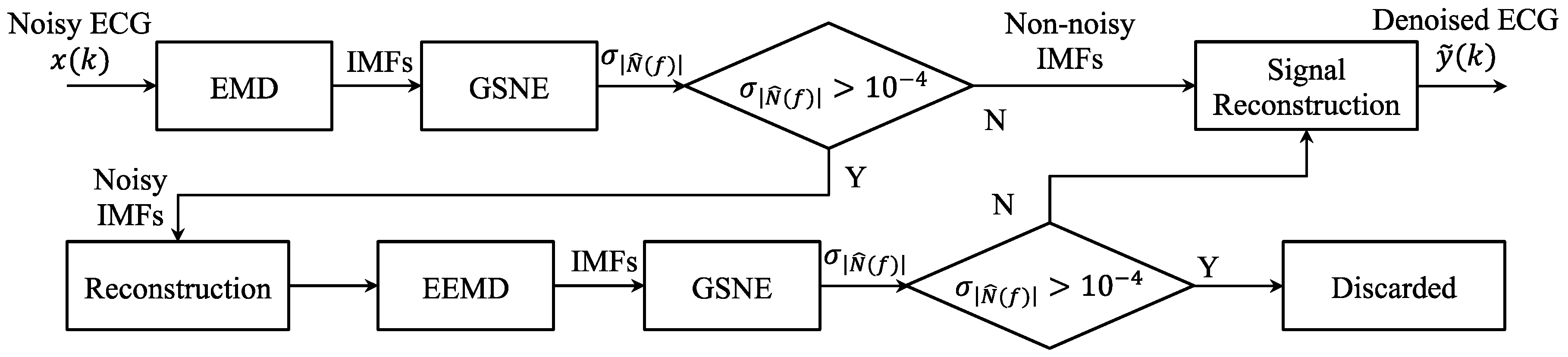
4. The Proposed GSNC Scheme
5. Results
5.1. Effect of White Noise in the EEMD
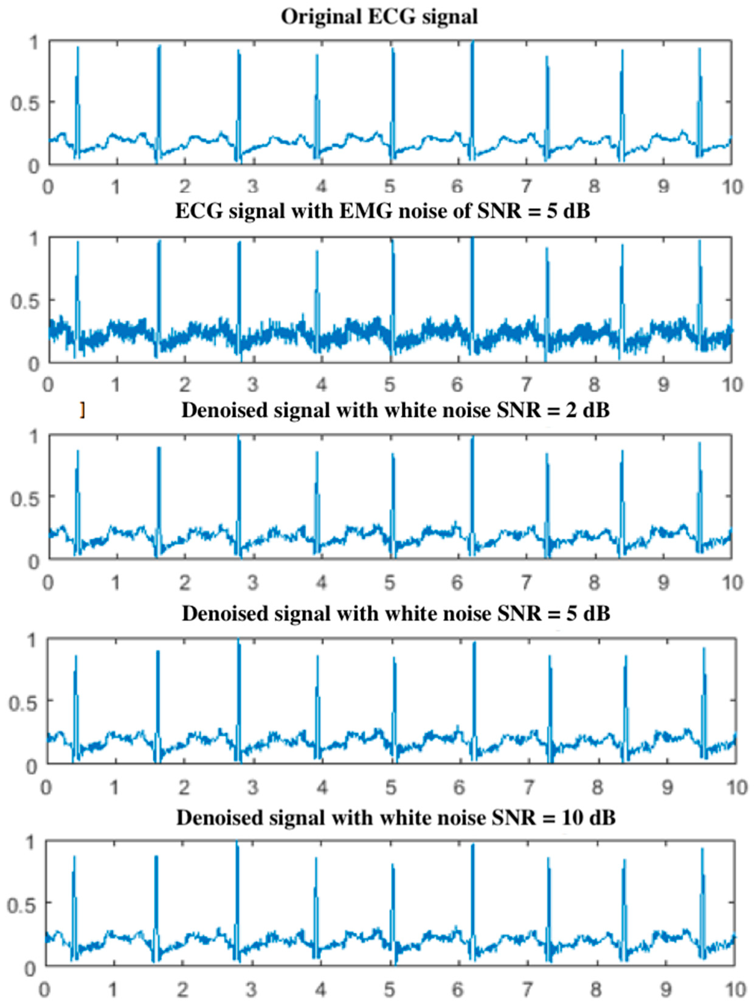
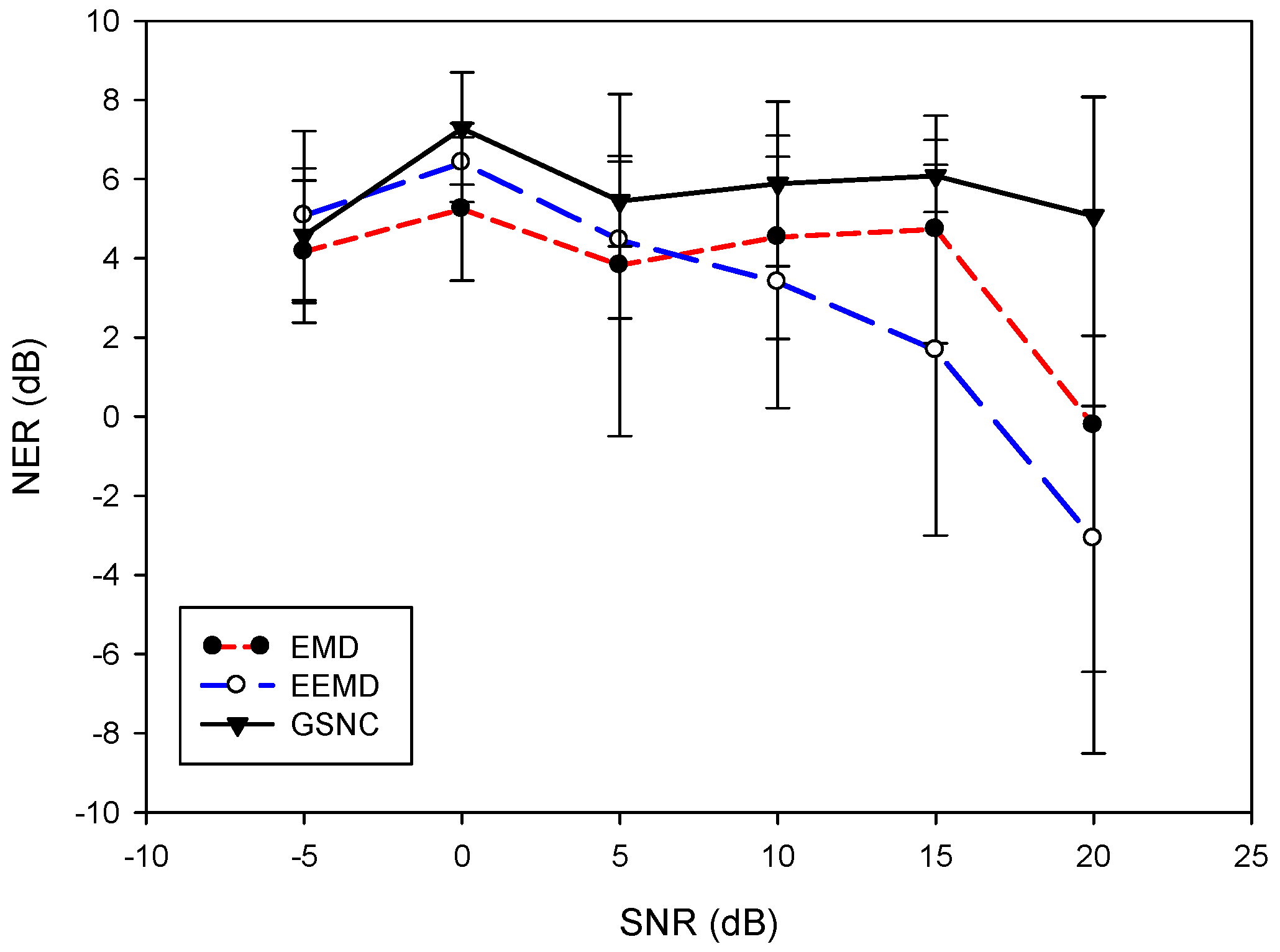
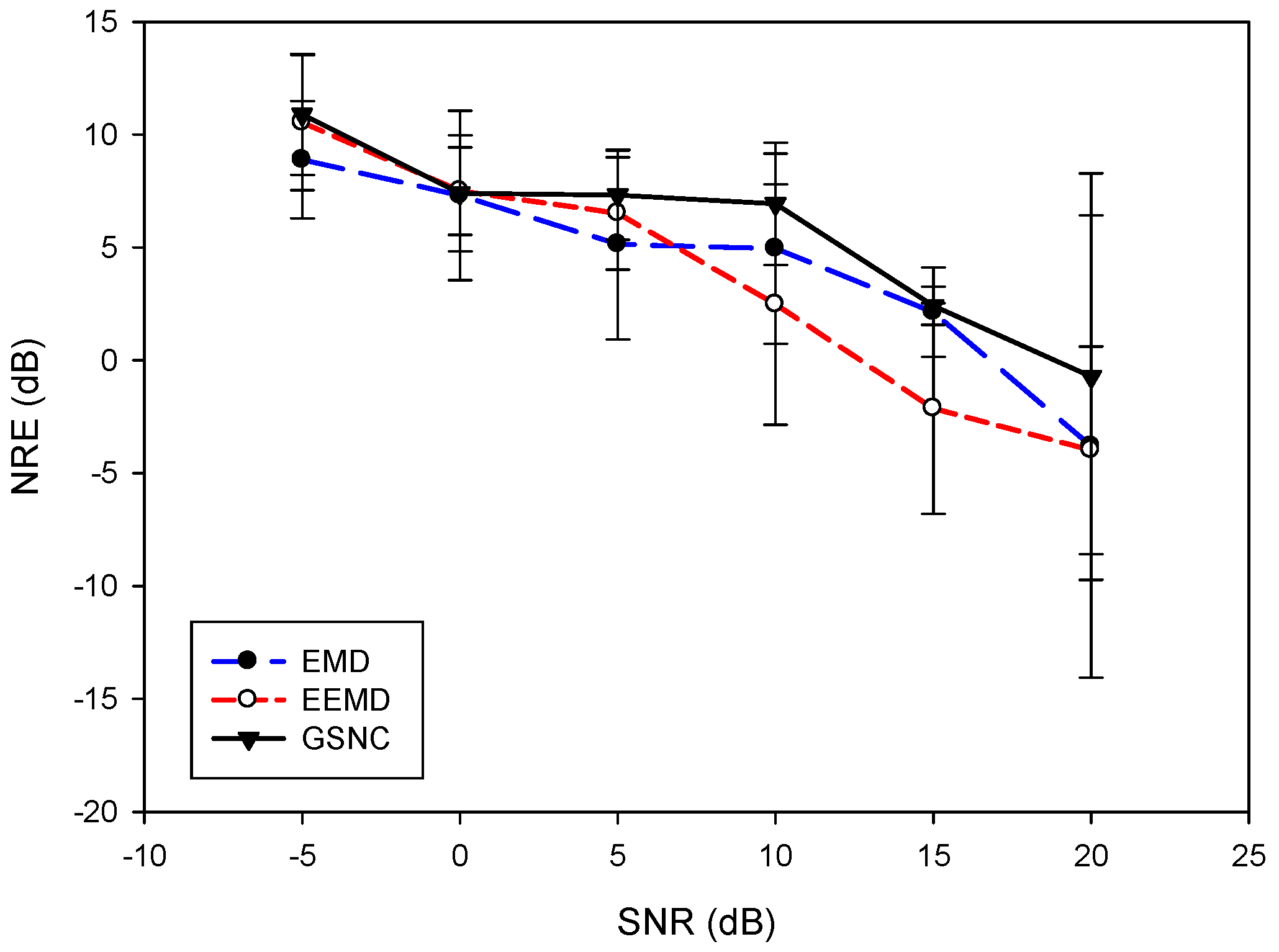
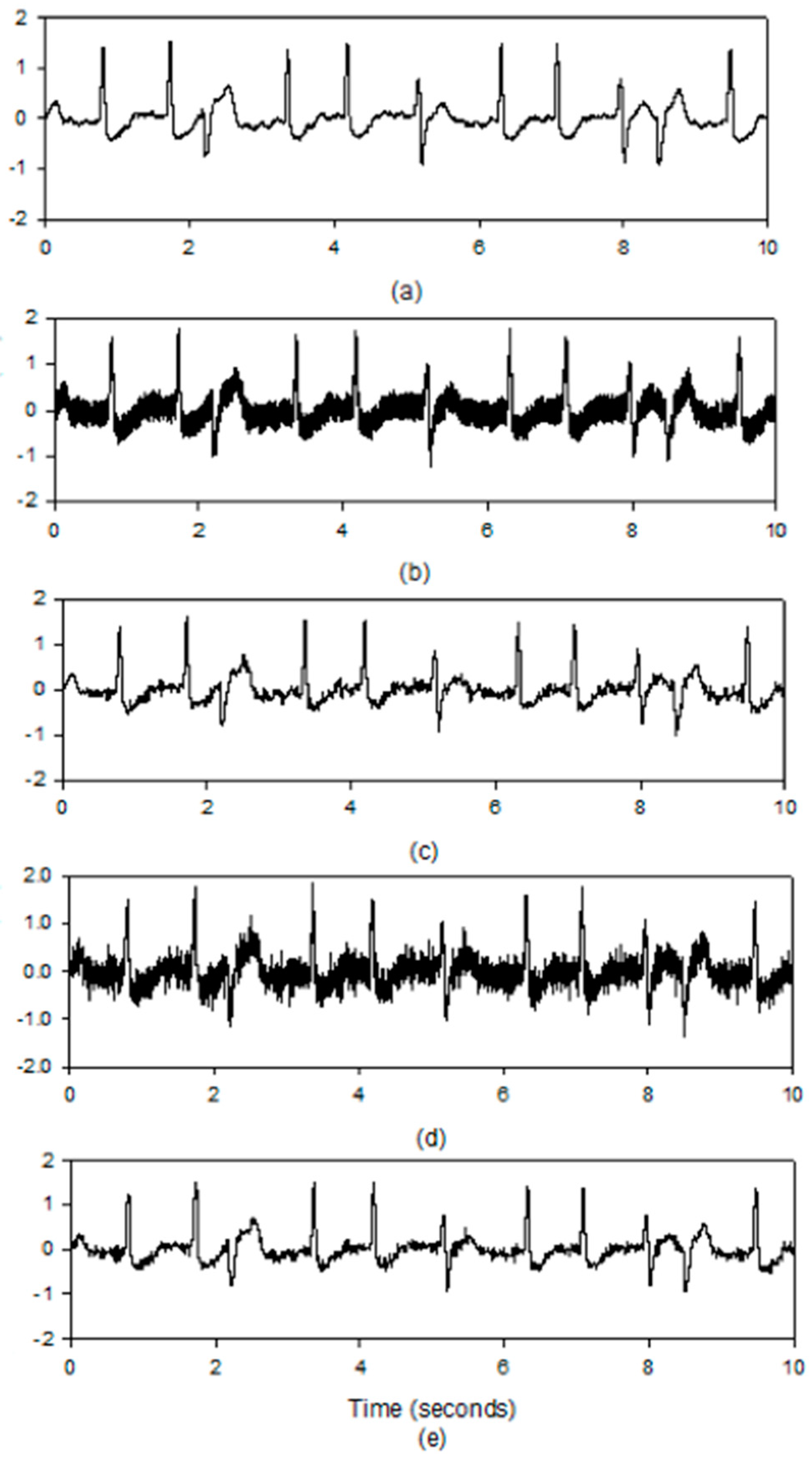
5.2. Results for the PLn and EMG Noise
6. Discussion
7. Conclusions
Author Contributions
Funding
Conflicts of Interest
References
- Holter Monitor. Available online: http://www.heart.org/HEARTORG/Conditions/HeartAttack/SymptomsDiagnosisofHeartAttack/Holter-Monitor_UCM_446437_Article.jsp#.Vxlo9nlJnGI (accessed on 20 December 2018).
- Cardiac Event Recorder. Available online: http://www.heart.org/HEARTORG/Conditions/Arrhythmia/PreventionTreatmentofArrhythmia/C ardiac-Event-Recorder_UCM_447317_Article.jsp#.VxloV3lJnGI (accessed on 20 December 2018).
- Liu, S.-H.; Wang, J.-J.; Su, C.-H.; Tan, T.-H. Development of a patch-type electrocardiographic monitor for real time heartbeat detection and heart rate variability analysis. J. Med Biol. Eng. 2018, 38, 411–423. [Google Scholar] [CrossRef]
- Pan, J.; Tompkins, W.J. A real-time QRS detection algorithm. IEEE Trans. Biomed. Eng. 1985, BME-32, 230–236. [Google Scholar] [CrossRef]
- Friesen, G.M.; Jannett, T.C.; Jadallah, M.A.; Yates, S.L.; Quint, S.R.; Troynagle, H. A comparison of the noise sensitivity of nine QRS detection algorithms. IEEE Trans. Biomed. Eng. 1990, 37, 85–98. [Google Scholar] [CrossRef] [PubMed]
- Slonim, T.; Slonim, M.; Ovsyscher, E. The use of simple FIR filters for filtering of ECG signals and a new method for post-filter signal reconstruction. Int. Proc. Comput. Cardiol. 1993, 871–873. [Google Scholar]
- Liu, S.-H. Motion artifact reduction in electrocardiogram using adaptive filter. J. Med Biol. Eng. 2011, 31, 67–72. [Google Scholar] [CrossRef]
- Thakor, N.; Zhu, Y. Applications of adaptive filtering to ECG analysis: Noise cancellation and arrhythmia detection. IEEE Trans. Biomed. Eng. 1991, 38, 785–794. [Google Scholar] [CrossRef]
- Sankar, A.B.; Kumar, D.; Seethalakshmi, K. Performance study of various adaptive filter algorithms for noise cancellation in respiratory signals. Signal Process. Int. J. 2010, 4, 267–278. [Google Scholar]
- Augustyniak, P. Time–frequency modelling and discrimination of noise in the electrocardiogram. Physiol. Meas. 2003, 24, 1–15. [Google Scholar] [CrossRef]
- Rundo, F.; Conoci, S.; Ortis, A.; Battiato, S. An advanced bio-inspired photoplethysmography (PPG) and ECG pattern recognition system for medical assessment. Sensors. 2018, 18, 405. [Google Scholar] [CrossRef]
- Erçelebi, E. Electrocardiogram signals de-noising using lifting-based discrete wavelet transform. Comput. Biol. Med. 2004, 34, 479–493. [Google Scholar] [CrossRef]
- Blanco-Velasco, M.; Weng, B.; Barner, K.E. ECG signal denoising and baseline wander correction based on the empirical mode decomposition. Comput. Biol. Med. 2008, 38, 1–13. [Google Scholar] [CrossRef] [PubMed]
- Chang, K.-M.; Liu, S.-H. Gaussian noise filtering from ECG by Wiener filter and ensemble empirical mode decomposition. Signal Process. Syst. 2011, 64, 249–264. [Google Scholar] [CrossRef]
- Wu, Z.; Huang, N.E. A study of the characteristics of white noise using the empirical mode decomposition method. Int Proc. R. Soc. 2004, 460, 1597–1611. [Google Scholar] [CrossRef]
- Wu, Z.; Huang, N.E. Ensemble empirical mode decomposition: A noise-assisted data analysis method. Adv. Adapt. Data Anal. 2009, 1, 1–41. [Google Scholar] [CrossRef]
- Liu, S.H.; Chang, K.M.; Cheng, D.C. The progression of muscle fatigue during exercise estimation with the aid of high-frequency component parameters derived from ensemble empirical mode decomposition. IEEE J. Biomed. Health Inf. 2014, 18, 1647–1658. [Google Scholar] [CrossRef] [PubMed]
- Wu, H.-T.; Lee, C.-H.; Sun, C.-K.; Hsu, J.-T.; Huang, R.-M.; Tang, C.-J. Arterial waveforms measured at the wrist as indicators of diabetic endothelial dysfunction in the elderly. IEEE Trans. Instrum. Meas. 2012, 61, 162–169. [Google Scholar] [CrossRef]
- Jebaraj, J.; Arumugam, R. Ensemble empirical mode decomposition-based optimised power line interference removal algorithm for electrocardiogram signal. IET Signal Process. 2016, 10, 583–591. [Google Scholar] [CrossRef]
- Kopsinis, Y.; McLaughlin, S. Development of EMD-Based denoising methods inspired by wavelet thresholding. IEEE Trans. Signal Process. 2009, 57, 1351–1362. [Google Scholar] [CrossRef]
- Kumaravel, N.; Nithiyanandam, N. Genetic-algorithm cancellation of sinusoidal power line interference in electrocardiograms. Med. Biol. Eng. Comput. 1998, 36, 191–196. [Google Scholar] [CrossRef]
- Deng, J.L. Control problems of grey system. Syst. Control Lett. 1982, 1, 288–294. [Google Scholar]
- Deng, J.L. Introduction to grey system theory. J. Grey Syst. 1989, 1, 1–24. [Google Scholar]
- Massachusetts Institute of Technology. MIT-BIH Database Distribution; Massachusetts Institute of Technology: Cambridge, MA, USA, 1998. [Google Scholar]
- Kammler, D.W. A First Course in Fourier Analysis; Prentice-Hall: Upper Saddle River, NJ, USA, 2000; p. 74. [Google Scholar]


| mitdb/100 | mitdb/105 | mitdb/108 | mitdb/203 | mitdb/223 | mitdb/228 | ||
|---|---|---|---|---|---|---|---|
| IMF 1 | 1.16 × 10⁻⁴ | 7.90 × 10⁻⁵ | 6.97 × 10⁻⁵ | 8.37 × 10⁻⁵ | 1.27 × 10⁻⁴ | 7.84 × 10⁻⁵ | |
| 2.56 × 10⁻³ | 4.54 × 10⁻³ | 2.78 × 10⁻³ | 4.40 × 10⁻³ | 6.39 × 10⁻³ | 2.60 × 10⁻³ | ||
| IMF 2 | 5.18 × 10⁻⁵ | 3.91 × 10⁻⁵ | 2.93 × 10⁻⁵ | 4.23 × 10⁻⁵ | 5.065 × 10⁻⁵ | 3.24 × 10⁻⁵ | |
| 6.58 × 10⁻⁴ | 1.22 × 10⁻³ | 6.52 × 10⁻⁴ | 1.13 × 10⁻³ | 1.61 × 10⁻³ | 6.81 × 10⁻⁴ | ||
| IMF 3 | 2.66 × 10⁻⁵ | 3.05 × 10⁻⁵ | 1.70 × 10⁻⁵ | 2.37 × 10⁻⁵ | 2.98 × 10⁻⁵ | 1.57 × 10⁻⁵ | |
| 2.08 × 10⁻⁴ | 3.51 × 10⁻⁴ | 2.06 × 10⁻⁴ | 3.31 × 10⁻⁴ | 4.85 × 10⁻⁴ | 2.02 × 10⁻⁴ | ||
| IMF 4 | 1.43 × 10⁻⁵ | 1.36 × 10⁻⁵ | 9.01 × 10⁻⁶ | 1.25 × 10⁻⁵ | 2.51 × 10⁻⁵ | 7.02 × 10⁻⁶ | |
| 8.93 × 10⁻⁵ | 1.01 × 10⁻⁴ | 6.09 × 10⁻⁵ | 1.05 × 10⁻⁴ | 1.65 × 10⁻⁴ | 5.63 × 10⁻⁵ | ||
| IMF 5 | 6.58 × 10⁻⁶ | 6.85 × 10⁻⁶ | 5.22 × 10⁻⁶ | 7.67 × 10⁻⁶ | 1.12 × 10⁻⁵ | 3.80 × 10⁻⁶ | |
| 3.28 × 10⁻⁵ | 4.26 × 10⁻⁵ | 2.40 × 10⁻⁵ | 3.59 × 10⁻⁵ | 6.25 × 10⁻⁵ | 2.61 × 10⁻⁵ | ||
| mitdb/100 | mitdb/105 | mitdb/108 | mitdb/203 | mitdb/223 | mitdb/228 | ||
|---|---|---|---|---|---|---|---|
| IMF 1 | 1.16 × 10⁻⁴ | 7.90 × 10⁻⁵ | 6.97 × 10⁻⁵ | 8.37 × 10⁻⁵ | 1.27 × 10⁻⁴ | 7.84 × 10⁻⁵ | |
| 1.36 × 10⁻³ | 2.51 × 10⁻³ | 1.43 × 10⁻³ | 2.37 × 10⁻³ | 3.42 × 10⁻³ | 1.37 × 10⁻³ | ||
| IMF 2 | 5.18 × 10⁻⁵ | 3.91 × 10⁻⁵ | 2.93 × 10⁻⁵ | 4.23 × 10⁻⁵ | 5.06 × 10⁻⁵ | 3.24 × 10⁻⁵ | |
| 4.00 × 10⁻⁴ | 7.75 × 10⁻⁴ | 4.75 × 10⁻⁴ | 7.04 × 10⁻⁴ | 1.03 × 10⁻³ | 4.82 × 10⁻⁴ | ||
| IMF 3 | 2.66 × 10⁻⁵ | 3.05 × 10⁻⁵ | 1.70 × 10⁻⁵ | 2.37 × 10⁻⁵ | 2.98 × 10⁻⁵ | 1.57 × 10⁻⁵ | |
| 1.40 × 10⁻⁴ | 2.06 × 10⁻⁴ | 1.30 × 10⁻⁴ | 2.09 × 10⁻⁴ | 3.17 × 10⁻⁴ | 1.20 × 10⁻⁴ | ||
| IMF 4 | 1.43 × 10⁻⁵ | 1.36 × 10⁻⁵ | 9.01 × 10⁻⁶ | 1.25 × 10⁻⁵ | 2.5 × 10⁻⁵ | 7.02 × 10⁻⁶ | |
| 5.53 × 10⁻⁵ | 6.60 × 10⁻⁵ | 3.93 × 10⁻⁵ | 5.89 × 10⁻⁵ | 9.61 × 10⁻⁵ | 3.92 × 10⁻⁵ | ||
| IMF 5 | 6.58 × 10⁻⁶ | 6.85 × 10⁻⁶ | 5.22 × 10⁻⁶ | 7.67 × 10⁻⁶ | 1.12 × 10⁻⁵ | 3.80 × 10⁻⁶ | |
| 2.14 × 10⁻⁵ | 3.13 × 10⁻⁵ | 1.28 × 10⁻⁵ | 2.14 × 10⁻⁵ | 3.65 × 10⁻⁵ | 1.52 × 10⁻⁵ | ||
| Dataset | EMD | EEMD | GSNC | Dataset | EMD | EEMD | GSNC |
|---|---|---|---|---|---|---|---|
| mitdb/100 | −4.59 | 6.36 | 6.51 | mitdb/205 | 1.59 | −1.14 | 5.08 |
| mitdb/101 | 1.01 | 0.32 | 2.83 | mitdb/207 | 4.12 | 6.92 | 9.48 |
| mitdb/103 | −1.72 | 1.09 | 1.17 | mitdb/208 | −4.45 | 2.79 | −2.07 |
| mitdb/105 | 6.04 | 3.53 | 5.02 | mitdb/209 | −7.96 | −0.60 | −5.02 |
| mitdb/106 | −5.32 | 0.12 | −1.48 | mitdb/210 | 6.58 | 4.24 | 7.68 |
| mitdb/108 | 3.29 | 6.52 | 3.50 | mitdb/212 | −11.33 | −3.40 | −5.33 |
| mitdb/109 | 7.96 | 7.90 | 9.97 | mitdb/213 | 3.97 | −3.15 | 7.10 |
| mitdb/111 | 4.19 | 1.53 | 5.48 | mitdb/214 | −2.72 | 5.24 | −0.91 |
| mitdb/112 | 6.75 | 5.24 | 7.52 | mitdb/215 | −2.11 | 0.08 | 1.22 |
| mitdb/113 | −2.12 | −1.81 | −0.72 | mitdb/219 | −8.31 | 5.23 | 2.91 |
| mitdb/114 | −0.75 | 2.78 | 2.99 | mitdb/220 | −1.13 | −0.52 | 0.40 |
| mitdb/115 | −3.01 | −1.50 | 0.10 | mitdb/221 | 2.23 | 2.87 | 3.46 |
| mitdb/116 | −3.52 | 3.77 | 3.32 | mitdb/222 | 0.97 | −0.39 | 6.22 |
| mitdb/117 | 3.11 | 0.31 | 5.65 | mitdb/223 | 5.48 | 5.62 | 6.24 |
| mitdb/118 | −1.84 | −0.53 | −0.19 | mitdb/228 | 7.31 | 1.67 | 6.27 |
| mitdb/119 | 2.03 | 0.37 | 3.32 | mitdb/230 | −1.58 | 0.32 | −0.26 |
| mitdb/121 | 2.76 | 2.83 | 3.88 | mitdb/231 | −6.55 | −5.67 | −4.45 |
| mitdb/122 | 5.46 | 4.18 | 9.73 | mitdb/232 | −2.65 | 6.47 | 5.64 |
| mitdb/123 | −0.52 | −0.42 | −2.01 | mitdb/233 | 0.73 | 6.18 | 6.68 |
| mitdb/124 | 5.82 | 5.61 | 6.74 | mitdb/234 | −5.21 | 0.66 | −0.22 |
| mitdb/201 | −12.83 | 5.44 | 6.72 | ||||
| mitdb/202 | 7.83 | 4.53 | 8.42 | Mean | 0.10 | 2.20 | 3.34 |
| mitdb/203 | 5.40 | 3.07 | 5.15 | Std. | 5.21 | 3.21 | 4.03 |
| Dataset | EMD | EEMD | GSNC | Dataset | EMD | EEMD | GSNC |
|---|---|---|---|---|---|---|---|
| mitdb/100 | −3.02 | 8.66 | 7.94 | mitdb/205 | 1.71 | 1.91 | 10.87 |
| mitdb/101 | 0.14 | 2.18 | 2.65 | mitdb/207 | 11.32 | 12.47 | 13.21 |
| mitdb/103 | −2.79 | 1.70 | 0.77 | mitdb/208 | −2.11 | 6.44 | 2.81 |
| mitdb/105 | 6.44 | 7.68 | 8.21 | mitdb/209 | 0.31 | −1.44 | 1.65 |
| mitdb/106 | 5.03 | 2.21 | 5.42 | mitdb/210 | 7.79 | 3.66 | 9.50 |
| mitdb/108 | 6.61 | 7.39 | 3.87 | mitdb/212 | −1.29 | −4.15 | −5.14 |
| mitdb/109 | 10.84 | 11.17 | 12.61 | mitdb/213 | 2.55 | 7.52 | 5.96 |
| mitdb/111 | 8.23 | 3.79 | 9.44 | mitdb/214 | 7.64 | 4.59 | 10.04 |
| mitdb/112 | 1.50 | 3.16 | 1.97 | mitdb/215 | 2.13 | 0.14 | 3.66 |
| mitdb/113 | −0.92 | 1.76 | 1.43 | mitdb/219 | 7.62 | 4.16 | 9.44 |
| mitdb/114 | 4.96 | 9.50 | 12.16 | mitdb/220 | 0.42 | −1.53 | 1.11 |
| mitdb/115 | 1.43 | −2.90 | −0.77 | mitdb/221 | 4.54 | 5.95 | 6.93 |
| mitdb/116 | 3.27 | 6.24 | 9.45 | mitdb/222 | 5.32 | 3.54 | 7.06 |
| mitdb/117 | −0.53 | −0.08 | 6.12 | mitdb/223 | 6.30 | 8.59 | 7.63 |
| mitdb/118 | −1.63 | −1.98 | −0.57 | mitdb/228 | 5.25 | 3.47 | 6.55 |
| mitdb/119 | 7.59 | 1.12 | 8.68 | mitdb/230 | 0.82 | 0.27 | 3.21 |
| mitdb/121 | 12.19 | 9.67 | 9.94 | mitdb/231 | −2.91 | −6.66 | −0.49 |
| mitdb/122 | 2.73 | 2.50 | 5.21 | mitdb/232 | −8.03 | 7.15 | 7.64 |
| mitdb/123 | 2.86 | −1.12 | 3.38 | mitdb/233 | 8.98 | 7.05 | 11.14 |
| mitdb/124 | 8.53 | 6.74 | 11.42 | mitdb/234 | −0.39 | 4.08 | 2.93 |
| mitdb/201 | 6.67 | 7.81 | 9.34 | ||||
| mitdb/202 | 4.10 | 7.98 | 9.79 | Mean | 3.52 | 3.85 | 6.14 |
| mitdb/203 | 9.21 | 3.26 | 9.72 | Std. | 4.52 | 4.27 | 4.29 |
© 2019 by the authors. Licensee MDPI, Basel, Switzerland. This article is an open access article distributed under the terms and conditions of the Creative Commons Attribution (CC BY) license (http://creativecommons.org/licenses/by/4.0/).
Share and Cite
Liu, S.-H.; Hsieh, C.-H.; Chen, W.; Tan, T.-H. ECG Noise Cancellation Based on Grey Spectral Noise Estimation. Sensors 2019, 19, 798. https://doi.org/10.3390/s19040798
Liu S-H, Hsieh C-H, Chen W, Tan T-H. ECG Noise Cancellation Based on Grey Spectral Noise Estimation. Sensors. 2019; 19(4):798. https://doi.org/10.3390/s19040798
Chicago/Turabian StyleLiu, Shing-Hong, Cheng-Hsiung Hsieh, Wenxi Chen, and Tan-Hsu Tan. 2019. "ECG Noise Cancellation Based on Grey Spectral Noise Estimation" Sensors 19, no. 4: 798. https://doi.org/10.3390/s19040798
APA StyleLiu, S.-H., Hsieh, C.-H., Chen, W., & Tan, T.-H. (2019). ECG Noise Cancellation Based on Grey Spectral Noise Estimation. Sensors, 19(4), 798. https://doi.org/10.3390/s19040798